Coulomb “blockade” of Nuclear Spin Relaxation in Quantum Dots

Abstract

We study the mechanism of nuclear spin relaxation in quantum dots due to the electron exchange with 2D gas. We show that the nuclear spin relaxation rate $T_{1}^{-1}$ is dramatically affected by the Coulomb blockade (CB) and can be controlled by gate voltage. In the case of strong spin-orbit (SO) coupling the relaxation rate is maximal in the CB valleys whereas for the weak SO coupling the maximum of $1/T_{1}$ is near the CB peaks.

Discreteness of energy spectra in quantum dots (QD), in combination with the Coulomb electron-electron interactions, determines all their physical properties [1]. In this paper, we study the impact of these two crucial features of QD on the interaction of electrons with nuclei. In particular, we evaluate nuclear spin relaxation (NSR) rate, $1/T_{1}$, which determines the effectiveness of dynamical nuclear spin polarization [2] as well.

What mechanisms of NSR are efficient in the QD? Because even weak magnetic fields suppress the NSR due to the dipole-dipole interaction of nuclear spins [2], we will consider NSR caused by the hyperfine coupling (HC) between nuclear, ${\bf S}$, and electron, $\sigma$ spins:

$${\cal H}_{h}=AV\sum\limits_{i}{\bf S}_{i}{\hat{\cal B}}({\bf r}_{i}),\quad{\hat{\cal B}}({\bf r}_{i})=\Psi_{\alpha}^{+}({\bf r}_{i})\mbox{\boldmath$\sigma$}_{\alpha\beta}\Psi_{\beta}({\bf r}_{i}),$$ (1)

where $A$ is the HC strength, and $V$ is the crystal cell volume. Substitution of the operator $\hat{{\cal B}}$ by its mean value, ${\bf{\cal B}}$, leads to the Hamiltonian of the system of nuclear spins, ${\bf S}_{i}$ in an effective magnetic field, ${\bf{\cal B}}$. Being uniform, this field causes only a uniform precession of ${\bf S}_{i}$, rather than NSR. Thermal fluctuations of ${\bf{\cal B}}$ in metals lead to the Korringa NSR mechanism [3] - each nuclear spin flip is accompanied by the creation of a triplet electron-hole pair.

In QD this process violates the energy conservation: the electron spectrum is discrete and Kramers degeneracy is lifted by the Overhauser nuclear field and/or external magnetic field. In order to overcome the mismatch of electron and nuclear spin splittings, a level broadening $\Gamma_{0}$ was included for electrons localized on donors [4, 5, 6] and in the quantum Hall effect regime [7, 8, 9]. However, $\Gamma_{0}$ must be introduced with a great caution. Indeed, any broadening implies that the final state of the system is not a discrete eigenstate of the QD but rather an eigenstate of a larger system with a continuous spectrum which includes QD as its subsystem. Thus, one has to specify the nature of the QD coupling to the outside world.

We propose that charge exchange between the QD and the reservoirs (with continuous spectrum) leads to NSR. Our main result is that NSR can be controlled and changed by orders of magnitude by the gate voltage, $V_{g}$, which defines the average number of the electrons in the QD. The origin of this effect is the Coulomb blockade (CB) [10] that determines the tunneling of electrons in and out of the QD. Furthermore, $1/T_{1}$ in QD is governed not only by the QD electrons tunneling rates and the effective fields ${\hat{\cal B}}({\bf r}_{i})$, but also by the probabilities for the QD to have a particular integer charge, $Q$, as well as by the occupation numbers of the electronic states in the QD and in the leads at a given $Q$. Moreover, we find that the NSR rate depends on the sensitivity of the QD spectrum to the change in the nuclear spin configuration, which is maximal in the presence of electron spin-orbit coupling (SOC).

Let us now discuss the role that SOC plays in NSR. Due to SOC the total spin of nuclei and electrons is not conserved. Each electron level, even if Kramers degeneracy is lifted, contains mixture of up and down spin states, and energy conservation law does not prevent nuclear spin flips (nuclear spin splitting $\hbar\omega\to 0$). Does the presence of SOC leads to NSR even in absolutely closed dots? The answer to this question is negative for the following reason. Due to SOC, both the magnitude, and the direction of the effective magnetic field, ${\bf{\cal B}}=<\hat{{\cal B}}>$, become spatially inhomogenous but remain time-independent.

Although the field originating from SOC, ${\bf{\cal B}}={\bf{\cal B}_{so}}({\bf r})$, causes an inhomogeneous spin precession and thus broadens the NMR line, it can not lead to the actual NSR. The reason is that ${\bf{\cal B}_{so}}({\bf r})$ is time-independent. One can separate this inhomogeneous spin precession by the spin echo technique [4]. Furthermore, a time-independent ${\bf{\cal B}}$ can reduce the nuclear polarization but is unable to eliminate it altogether. For example, if local nuclear polarization is parallel to ${\bf{\cal B}}$, it will not change at all.

However, even weak electron tunneling on and off the dot causes true NSR. The reason is that ${\bf{\cal B}}_{so}$ is determined by the particular electronic configuration, and is modified by each tunneling event, thus becoming time-dependent. This dynamics leads to NSR, because it is not reversible. Indeed, due to inhomogeneous precession of the nuclear spins, the adiabatic electron eigenstates change between tunneling events, and it is improbable that the system returns to the same electron/nuclear configuration.

Let us now roughly estimate the NSR rate due to this mechanism, given the effective electron escape rate $\gamma$. Typical rotation angle of ${\bf S}$ within the time $\gamma^{-1}$ is ${\cal B}_{so}/\gamma\ll 1$. At larger time scale, $t$, nuclear spins undergo random spin diffusion. The mean square angle deviation is $\langle\Theta^{2}(t)\rangle\sim({\cal B}_{so}/\Gamma)^{2}t\gamma={\cal B}_{so}^{2}t/\gamma$. Defining NSR rate $1/T_{1}$ by $\langle\Theta^{2}(T_{1})\rangle\sim 1$, we obtain $1/T_{1}\sim{\cal B}_{so}^{2}/\gamma$. The rate $\gamma$ can be fine tuned by adjusting the gate voltage, $V_{g}$, applied to the QD. $\gamma$ reaches maximum at the CB peak, where the dot conductance $G$ is maximal, and is minimal in the CB valley. We reach a counterintuitive conclusion: NSR rate peaks in the CB valleys, while near the CB peaks it is suppressed, see Fig.2. As we shall see, this conclusion holds as long as SOC is not too weak.

The described physical situation is not unique for NSR in QD. In particular, it resembles Mandelstam-Leontovich-Pollak-Geballe relaxation mechanisms of absorption of infrared radiation [12]: As long as the relaxation rate $\gamma_{r}$ exceeds the frequency of the radiation $\omega$, the relaxation rate is inverse proportional to $\gamma_{r}$. One can also recall the motional narrowing of spectral lines [13].

Our goal is the microscopic theory of NSR in QD which includes the calculation of $\gamma$ and ${\cal B}_{so}$. We start with the standard Hamiltonian of a QD connected to leads (see e.g. Ref. [1] for the discussion of its validity) $\hat{H}=\hat{H}_{D}+\hat{H}_{L}+\hat{H}_{LD}$, where $\hat{H}_{D}(t)$, $\hat{H}_{L}$ and $\hat{H}_{LD}$ describe, respectively, the dot, the leads and tunneling between them:

$$\hat{H}_{D}=\sum\nolimits_{\alpha\alpha}\epsilon_{\alpha}a^{\dagger}_{\alpha}a_{\alpha}+E_{c}\left(\hat{n}-{\cal N}\right)^{2},$$ (2)

$\hat{H}_{L}=\sum_{k,j}\epsilon_{k,j}b^{\dagger}_{k,j}b_{k,j},\hat{H}_{LD}=\sum_{k,j;\alpha}t_{\alpha}^{j}b^{\dagger}_{k,j}a_{\alpha}+h.c.$. Here $a_{\alpha},a^{\dagger}_{\alpha}$ and $b_{k,j,},b^{\dagger}_{k,j}$ are creation/annihilation electron operators describing single-electron QD states $\alpha$, and electrons in state $k$ in the lead $j$, respectively; $\hat{n}=\sum_{\alpha}a^{\dagger}_{\alpha}a_{\alpha}$ is the operator of the number of particles, ${\cal N}=CV_{g}/e$, $C$ is the capacitance of the dot, $e$ is the electron charge, and $E_{c}=e^{2}/2C$ is the single-electron charging energy; matrix elements $t_{\alpha}^{j}$ determine the tunneling widths of QD states $|\alpha\rangle$, $\Gamma_{t}^{(\alpha)}=\sum_{j}2\pi|t_{\alpha}^{j}|^{2}\nu$, where $\nu$ is the density of states in leads.

The NSR rate $1/T_{1}$ due to HC is connected to the linear response of the electronic system to Zeeman magnetic field induced by nuclei at their location [4]:

$$T_{1}^{-1}=2A^{2}V^{2}T{\rm Im}\chi_{xx}(\omega)/\omega|_{\omega\to 0}.$$ (3)

The transverse spin susceptibility $\chi_{xx}$ is defined by the response $\delta\langle s_{x}({\bf r})\rangle_{\omega}=\chi_{xx}(\omega)h_{\omega}$, $h_{\omega}=\int dt\exp{(i\omega t)}h(t)$, of the electron spin density, $s_{x}({\bf r})$, to the perturbation

$$\delta H=h(t)\sum\nolimits_{\alpha\beta}[s_{x}({\bf r})]_{\alpha\beta}a^{\dagger}_{\alpha}a_{\beta}.$$ (4)

As soon as SOC is included, the diagonal matrix elements $[s_{x}({\bf r})]_{\alpha\alpha}$, become finite and result in the shifts of the energy levels $\epsilon_{\alpha}$. We assume the dot to be weakly coupled to leads which are in thermodynamic equilibrium. Then the probability, $P_{j}$, for the QD electrons to be in the state $j$, tends to follow the Gibbs distribution $P_{j}^{G}$ determined by the instantaneous value of $\hat{H}(t)$. However, $P_{j}$ is delayed as compared with $\hat{H}(t)$ due to finite relaxation:

$$P_{j}(t) = P_{j}^{G}\left\{\hat{H}(t)\right\}$$ (5)

$$- \sum_{k}\left[\int_{0}^{\infty}dt_{1}e^{-\hat{\Gamma}t_{1}}\right]_{jk}\frac{d}{dt}P_{k}^{G}\left\{\hat{H}(t)\right\}+\dots,$$ (6)

The matrix $\hat{\Gamma}$ characterizes the relaxation of the deviation of $P_{j}$ from their equilibrium values:

$$\frac{d}{dt}P_{j}(t)=-\sum_{k}\Gamma_{jk}P_{k},\quad\sum_{j}\Gamma_{jk}=\sum_{k}\Gamma_{jk}P_{k}^{G}=0.$$ (7)

The second term in the RHS of Eq. (5) gives rise to the relaxational dissipation [12]. The average spin equals to

$$\langle s_{x}({\bf r})\rangle=\sum\nolimits_{j\alpha}n_{\alpha}^{j}P_{j}s_{\alpha},\quad s_{\alpha}\equiv[s_{x}({\bf r})]_{\alpha\alpha}$$ (8)

where $n_{\alpha}^{j}=0,1$ is the occupation number of one-electron level $\alpha$ for a given state of the electron system $j$.

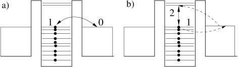
FIG. 1.: Processes dominating NSR in the (a) vicinity of and (b) away from the Coulomb blockade peaks. Lines denote single-electron levels. Dots indicate filled levels. Arrows show the relevant transition. Dashed lines in (b) show the actual electron processes leading to the relevant transition.

Substituting $P_{j}(t)$ into Eqs. (8) and Eq. (3), we obtain $\chi_{xx}(\omega)$ and $T_{1}^{-1}$:

$$\frac{1}{T_{1}}=-A^{2}V^{2}{T}\sum_{\alpha,\beta,j}s_{\alpha}\left[\int_{0}^{\infty}dt_{1}e^{-\hat{\Gamma}t_{1}}\right]_{\alpha j}\frac{\partial P^{G}_{j}}{\partial\epsilon_{\beta}}s_{\beta}.$$ (9)

We emphasize that this NSR rate is inversely proportional to the rate of the population relaxation of the QD states, provided the latter rate is larger than $\omega$.

As follows from Eq. (9), the NSR is dominated by electron configurations such that (i) their equilibrium probabilities are most sensitive to the shifts of one-electron levels, and (ii) their relaxation is slowest. Let us identify the optimal configurations for temperatures, $T$, below the mean level spacing, $\Delta$. We begin with $V_{g}$ tuned to a CB peak. The energy distance to the peak $U({\cal N})=E_{c}({\cal N}-N_{0})\simeq\Delta$, with $N_{0}$ being a half-integer closest to ${\cal N}$. Then the relaxation occurs (see Fig. 1a) via the two-level system (TLS) of the QD states with electron occupation numbers $N_{0}\pm 1/2$, which we denote $1$ and $0$ respectively. Occupation of other states is suppressed exponentially, i.e. $P_{0}+P_{1}=1$. The Gibbs distribution for such TLS gives $P_{1}^{G}/P_{0}^{G}=\exp\left[-(U({\cal N})+\epsilon_{1})/T\right]$ where $\epsilon_{1}$ is the energy of the filled electron level in state “1”. The relaxation matrix for the two states is determined by single tunneling width $\Gamma_{t}^{(1)}$

$$\hat{\Gamma}=\Gamma_{t}^{(1)}\pmatrix{1-f&-f\cr-1+f&f},$$ (10)

where $f=\{1+\exp[(U({\cal N})+\epsilon_{1})/T]\}^{-1}$ is the electron occupation number in the leads. From Eq. (9), we find

$$T_{1}^{-1}=\frac{A^{2}V^{2}|[s({\bf r})_{x}]_{11}|^{2}}{4\hbar\Gamma_{t}}\cosh^{-2}\frac{|U({\cal N})|+\epsilon_{1}}{2T}.$$ (11)

Thus, NSR decreases rapidly as $V_{g}$ deviates from the CB peaks, because the sensitivity of $P_{j}$ to $\epsilon_{\alpha}$ is exponentially suppressed by lifting the charge degeneracy.

Naively, one may expect the Eq. (11) to hold, at least qualitatively, even far from the peaks. However, as soon as $|U({\cal N})|$ exceeds $\Delta$, another TLS becomes optimal, see Fig. 1b. The energy difference between the two configurations in this TLS (we will call them $1$ and $2$) is $\epsilon_{eh}$ – the smallest energy of the electron-hole pair excited in the dot. At $|U({\cal N})|\gtrsim\Delta$, $\epsilon_{eh}<|U({\cal N})|$, the population of all other states is negligible. As a result, $P_{1}+P_{2}=1$. In the equilibrium, $P_{2}^{G}/P_{1}^{G}=\exp\left[-(\epsilon_{2}(t)-\epsilon_{1}(t))/T\right]$, i.e. in contrast with the previous case $P_{1,2}$ are $|U(N)|$-independent because now the relevant excitation does not change the charge of the QD. Charging energy, however, determines the rate of the transitions between the two states. If $V_{g}$ is not too far from the peak, $U({\cal N})\lesssim T\ln(E_{C}^{2}/\Gamma_{T}\Delta)$, the transition $1\to 2$ proceeds via the state $0$ (i.e. due to electron transfer between the QD and the reservoir) as an intermediate real state. One finds

$$\hat{\Gamma}=\frac{\Gamma_{t}^{(1)}\Gamma_{t}^{(2)}e^{-\frac{|U({\cal N}|)}{T}}}{\Gamma_{t}^{(1)}+\Gamma_{t}^{(2)}}\pmatrix{e^{\frac{\epsilon_{1}}{T}};&-e^{\frac{\epsilon_{2}}{T}}\cr-e^{\frac{\epsilon_{1}}{T}};&e^{\frac{\epsilon_{2}}{T}}}.$$ (13)

This result can be derived from the master equation including the state $0$. For its interpretation consider the rate of the $1\to 2$ transition, $[\hat{\Gamma}]_{11}$. The electron escape rate out of the state $1$ is $\Gamma_{t}^{(1)}e^{-\frac{|U({\cal N})|+\epsilon_{1}}{T}}$. After the electron leaves the QD, another one enters during the time $\simeq 1/\Gamma_{t}$. It occupies the state $2$ with the probability $\Gamma_{t}^{(2)}/(\Gamma_{t}^{(1)}+\Gamma_{t}^{(2)})$. The product of those two factors gives the probability of the transition $1\to 2$.

At larger deviations from the CB peak, $|U({\cal N})|\gtrsim T\ln(E_{c}^{2}/\Gamma_{t}\Delta)$, processes changing the QD charge can be neglected. The relaxation is now determined by the inelastic co-tunneling mechanism [11, 1], i.e., the state $0$ is used as a virtual state. The Eq. (13) becomes

$$\hat{\Gamma}=\frac{\Gamma_{t}^{(1)}\Gamma_{t}^{(2)}\epsilon_{21}}{4\pi\left[U({\cal N})\right]^{2}}\left[\pmatrix{F-1&-F-1\cr-F+1&F+1}\right],$$ (14)

where $\epsilon_{21}=\epsilon_{2}-\epsilon_{1}>0$, is the lowest energy of the electron-hole excitation in the QD, $F=\coth(\epsilon_{21}/2T)$. The factors in parenthesis are determined by the phase volume for the electron-hole pair created in the reservoir as the result of the inelastic co-tunneling process.

Using the equilibrium occupation numbers of the two QD states and Eqs. (14) and (9), we find

$$T_{1}^{-1} = \frac{A^{2}V^{2}|[s({\bf r})_{x}]_{11}-[s({\bf r})_{x}]_{22}|^{2}}{4\hbar\ {\rm max}\ (\Gamma_{t},\Gamma_{c})\cosh^{2}\frac{\epsilon_{21}}{2T}}$$ (15)

$$\Gamma_{t} = \frac{2\Gamma_{t}^{(1)}\Gamma_{t}^{(2)}\cosh\frac{\epsilon_{21}}{2T}}{\Gamma_{t}^{(1)}+\Gamma_{t}^{(2)}}e^{-\frac{|U({\cal N})|}{T}};$$ (16)

$$\Gamma_{c} = \frac{\Gamma_{t}^{(1)}\Gamma_{t}^{(2)}\epsilon_{21}\coth\frac{\epsilon_{21}}{2T}}{2\pi\left[U({\cal N})\right]^{2}}.$$ (17)

This result qualitatively differs from Eq. (11), and the dependence of $1/T_{1}$ on $V_{g}$ is non-trivial, see Fig. 2.

FIG. 2.: Sketch of the predicted NSR dependence on $V_{g}$ in the presence of SOC. Dashed line shows the linear conductance through the dot.

With yet further change of $V_{g}$ towards the bottom of a CB valley, one has to take into account the state $0$ with an electron removed from the dot (hole-like process) and with an electron added to the dot (electron-like process). This changes the rates $\Gamma_{t,c}$ in Eq. (15):

$$\Gamma_{t} = \frac{4\Gamma_{t}^{(1)}\Gamma_{t}^{(2)}\cosh\frac{\epsilon_{21}}{2T}e^{-E_{C}/T}}{\Gamma_{t}^{(1)}+\Gamma_{t}^{(2)}}\cosh\frac{|U({\cal N})|-E_{C}}{T};$$ (18)

$$\Gamma_{c} = \frac{\Gamma_{t}^{(1)}\Gamma_{t}^{(2)}\epsilon_{21}\coth\frac{\epsilon_{21}}{2T}}{2\pi}\left[\frac{1}{|U({\cal N})|}-\frac{1}{2E_{C}-|U({\cal N})|}\right]^{2}.$$ (19)

Note that the inelastic rate $\Gamma_{c}$ vanishes at the bottom of the valley, because the electron- and hole-like processes with the same final states are coherent, and their amplitudes are opposite in sign due to the Fermi statistics (the higher levels would give non-zero contribution, but the conclusion about the maximum of $1/T_{1}$ at the bottom of the CB valley remains valid). Overall dependence of $1/T_{1}$ on $V_{g}$ in the presence of SOC is sketched on Fig. 2.

We now discuss NSR when SOC of electrons in QD is absent, and each QD level corresponds to a spin projection aligned or antialigned with magnetic field. For typical distance between the lowest unoccupied QD level level and highest occupied QD level with opposite spin, $\epsilon_{2}-\epsilon_{1}\sim\Delta\gg\Gamma^{(i)},T$, the calculation of the susceptibility $\chi_{xx}(\omega)$ is equivalent to the evaluation of the Fermi golden rule probability of the simultaneous electron and nuclear spin flip. In this process, the initial and final electron states are real, one or both of them are in the reservoir, and energy-nonconserving electron spin flip inside the QD is incorporated as the virtual transition.

In the vicinity of the CB peaks, the two relevant QD states are electron on the lower level (1) and electron in the leads (2), see Fig. 3. Deeper in the valleys the main contribution is due to the process analogous to the elastic cotunneling in the CB valley conductance (Fig. 3b): the initial and final QD electron configurations coincide but the electron-hole triplet pair with is excited in the leads.

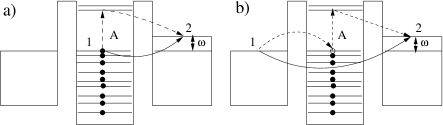
FIG. 3.: Dominant NSR processes at weak SOC in the (a) vicinity of and (b) away from the CB peaks ($\epsilon_{2}-\epsilon_{1}\gg\Gamma^{(i)}$). Solid lines with arrows denote transitions between initial and final states, dashed lines with arrows correspond to stages of those transitions. The spin flips occur in transitions “A”.

The result for the overall NSR rate dependence on $V_{g}$ in the absence of SOC is

$$\frac{1}{T_{1}}=\frac{A^{2}V^{2}|[s({\bf r})_{x}]_{12}|^{2}\Gamma_{t}^{(2)}\left(\epsilon_{1}-\epsilon_{2}\right)^{-2}}{2\hbar{\rm\min}\left(\cosh^{-2}\frac{|U({\cal N})|+\epsilon_{1}}{2T},\ \frac{\pi\left[U({\cal N})\right]^{2}}{\Gamma_{t}^{(1)}T}\right)}$$ (20)

Such NSR rate [14] is directly proportional to the rate of the population relaxation of the QD states, is maximal at CB peaks, minimal in the valley, and much smaller than $1/T_{1}$ in the presence of SOC.

We now estimate the NSR rate. In GaAs, $A\!=40\mu$eV[6], and $V\!=\!45\AA^{3}$. We consider QD formed in a 50Å-wide quantum well, with $0.1\mu$m in-plane dimensions, charging energy $E_{c}=0.5$meV, level spacing $\Delta=50\mu$eV, and tunneling width $\Gamma_{t}\!=\!2\mu$eV, at $T=100$mK. The typical matrix element $s_{11}$ is of the order of the inverse volume of the dot. Therefore we use $V^{2}s_{11}^{2}=0.8\times 10^{-12}$ in Eq. (11), and obtain $T_{1}^{-1}=0.25$Hz at the CB peak, and $T_{1}^{-1}=2\times 10^{-3}$Hz in the NSR minimum close to the CB peak, at $U({\cal N})\!=\!55\mu$eV, Fig.2. In the CB valley, by using Eq. (15,19), and assuming $s_{11}\!-\!s_{22}\sim 0.1s_{11}$, at $U({\cal N})=0.495$meV we obtain $T_{1}^{-1}=1.6\times 10^{3}$Hz. Our analysis shows also that even for QD with rather weak SOC, $T_{1}^{-1}$ in the CB valley has at least local maximum, so that the minimal NSR rate occurs at $V_{g}$ values between the CB peak and the CB valley bottom. Thus, $V_{g}$ indeed changes $T_{1}^{-1}$ by orders of magnitude.

In conclusion, we have shown that nuclear spin relaxation in QD is strongly affected by the Coulomb blockade, as well as the spin-orbit coupling, and proposed the relaxational mechanism of NSR. The NSR rate is predicted to have non-trivial dependence on $V_{g}$. Similarly to nuclei in experiments on quantum point contacts [15], nuclei shall affect transport properties of QD. The gate voltage depedence of NSR can be used, in particular, for creating and sustaining nuclear spin polarization in QD for electron spin filtering (we are grateful to C.M. Marcus for discussions of this experimental setting). This work was supported by DARPA QUIST program (Y.L.-G.) and (B.A.) and by Packard Foundation (I.A.).

REFERENCES

- [1] See I.L. Aleiner, P.W. Brouwer and L.I. Glazman, Phys. Reports, 358, 309 (2002) and references therein.
- [2] Optical Orientation, F. Meier and B.P. Zakharchenya, eds. (North Holland, Amsterdam, 1984).
- [3] J. Korringa, Physica 16 601 (1950).
- [4] A. Abragam, Principles of nuclear magnetism, Clarendon Press, Oxford (1961).
- [5] M. I. Dyakonov and V.I. Perel, Zh. Eksp. Teor. Fiz., 65, 362 (1973) [ Sov. Phys. JETP., 38, 177 (1973)].
- [6] D. Paget et al., Phys. Rev. B 15 5780 (1977).
- [7] A. Berg, et al., Phys. Rev. Lett., 64 2563 (1990).
- [8] I. D. Vagner and T. Maniv, Physica B, 204 141 (1995).
- [9] D. Antoniou and A.H. Macdonald, Phys. Rev. B 43 11686 (1991).
- [10] D. V. Averin and K. K. Likharev, in Mesoscopic Phenomena in Solids, eds B. L. Altshuler, P. A. Lee and R. A. Webb (North Holland, Amsterdam, 1991).
- [11] D. V. Averin and Y. V. Nazarov, Phys. Rev. Lett., 65, 2446 (1990); D. V. Averin and A. A. Odintsov, Phys. Lett. A, 140 251 (1989).
- [12] L. D. Landau and E.M. Lifshitz, Fluid Mechanics (Pergamon, Oxford, 1977); M. Pollak and T.H. Geballe, Phys. Rev., 122 1742 (1961).
- [13] P. W. Anderson, Journ. Phys. Sc. J. 9 316 (1954).
- [14] We note that when QD levels relevant for NSR are anomalously close, and SOC is absent, the Fermi golden rule approach Eq. (20) cannot be used. This situation occurs when the Zeeman effect brings distinct orbital states close to each other. The probability of such events is small, . The NSR rate in this case is caused by shifts of QD energy levels due to HC, Eq. (4), and is determined by using Eq. (9). The resulting NSR rate is described by the equations similar to Eqs.(11,15,19), and has the same -dependence as NSR at strong SOC. (In order to use these equations in the absence of SOC, one has to introduce the rotated basis of spinors in which matrix elements are non-zero).
- [15] K. R. Wald et al., Phys. Rev. Lett., 73 1011 (1994).