Kondo and anti-Kondo resonances in transport through nanoscale devices

Abstract

We study the current through a quantum wire side coupled to a quantum dot, and compare it with the case of an embedded dot. The system is modeled by the Anderson Hamiltonian for a linear chain, with one atom either coupled to (side-dot) or substituted by (embedded dot) a magnetic impurity. For realistic (small) hopping of the dot to the rest of the system, an exact relationship between both conductivities holds. We calculate the temperature dependence for moderate values of the Coulomb repulsion $U$ using an interpolative perturbative scheme. For sufficiently large $U$ and temperature greater than the Kondo temperature, the conductance as a function of gate voltage displays two extrema.

]

I Introduction

Transport through quantum dots have been studied in a series of recent experiments,[1, 2, 3] in which the peculiar features of the spectral density in the Kondo effect are manifested. An important fact in these experiments is that only one Kondo impurity is present.

While these experiments correspond to embedded quantum dots, very recent studies provide predictions for other situations, in particular a quantum dot side coupled to a quantum wire.[4, 5, 6] In Refs. 4 and 5, decoupling approximations were used for infinite Coulomb repulsion $U,$ which have limitations at finite temperatures.[7] For example, in the slave-boson mean-field approximation,[5] there is an unphysical phase transition at which the impurity decouples from the rest of the system, either when the temperature $T=T_{K}$ (Kondo temperature) or for $\varepsilon_{F}-\varepsilon_{d}\gg\Delta$, where $\varepsilon_{F}$ is the Fermi energy, $\varepsilon_{d}$ is the impurity level and $\Delta=\Gamma/2$ is the half-width half-maximum of the resonant level.[8] The method used by Torio et al. is expected to be very accurate,[6, 9] but it is limited to $T=0.$

Here we report calculations of the conductance as a function of temperature and gate voltage for embedded and quantum dots for $U\leq 8\Delta.$ In some experimental situations $\Delta\sim 0.15$ meV, $U\sim 0.6$ meV.[1, 3] Thus, this work complements previous ones for infinite $U$ or $T=0$, and presents a more systematic study of the temperature dependence for moderate $U$. We use second-order perturbation theory in $U$[10, 11, 12] modified to ensure that the approximation is exact in different limits, including $U\rightarrow+\infty.$[13, 14, 15]

The paper is organized as follows. In section II we write the relevant expressions which relate the conductance with the spectral density at the dot. The approximation for the latter is briefly reviewed and discussed in section III. Section IV contains the main results. Section V contains a brief summary and discussion.

II Conductance for embedded and side dots

For both cases, the Hamiltonian can be written as an Anderson model

$$H=H_{0}+H_{con},$$ (1)

where $H_{0}$ describes a tight-binding chain without site $0$ plus a disconnected quantum dot, and $H_{con}$ contains the hopping terms which connect the quantum dot with the chain,

$$H_{0}=-t\sum_{\sigma,i\neq 0,1}\left(c_{i\sigma}^{\dagger}c_{i-1\sigma}+H.c.\right)+\varepsilon_{d}\sum_{\sigma}d_{\sigma}^{\dagger}d_{\sigma}$$ (2)

$$+Ud_{\uparrow}^{\dagger}d_{\uparrow}d_{\downarrow}^{\dagger}d_{\downarrow}.$$ (3)

For the embedded dot,

$$H_{con}^{e}=-\sum_{\sigma}\left[d_{\sigma}^{\dagger}\left(t_{-1}^{\prime}c_{-1\sigma}+t_{1}^{\prime}c_{1\sigma}\right)+H.c.\right],$$ (4)

while for the side dot,

$$H_{con}^{s}=-\sum_{\sigma}\left[c_{0\sigma}^{\dagger}\left(t_{-1}c_{-1\sigma}+t_{1}c_{1\sigma}+t^{\prime}d_{\sigma}\right)+H.c.\right].$$ (5)

The conductance for an embedded dot can be written as[16]

$$G_{e}=\frac{2\pi e^{2}}{h}\sum_{\sigma}\int\left(-\frac{df}{d\omega}\right)\Gamma_{\sigma}(\omega)\rho_{d\sigma}(\omega),$$ (6)

where $f(\omega)$ is the Fermi function, $\rho_{d\sigma}(\omega)$ is the spectral density of the $d_{\sigma}$ states, and

$$\Gamma_{\sigma}(\omega)=\frac{\Gamma_{-1\sigma}(\omega)\Gamma_{1\sigma}(\omega)}{\Gamma_{-1\sigma}(\omega)+\Gamma_{1\sigma}(\omega)},\text{ with }\Gamma_{i\sigma}(\omega)=2\pi\left(t_{i}^{\prime}\right)^{2}\rho_{i\sigma}(\omega)$$ (7)

where $\rho_{i\sigma}(\omega)$ is the spectral density of the states described by the operators $c_{i\sigma}$ in $H_{0}.$ From the equations of motion for a semi-infinite chain, one easily obtains $\rho_{-1\sigma}=\rho_{1\sigma}=\left[1-(\omega/2t)^{2}\right]^{1/2}/\pi t.$ The resonant level width of the $d$ states is $\Delta_{\sigma}(\omega)=\pi\sum\limits_{i}\left(t_{i}^{\prime}\right)^{2}\rho_{i\sigma}(\omega).$ In the following we assume that $t_{i}^{\prime}$ is small, implying that the Kondo temperature is much smaller than the band width. The sum over spin indices reduces to a factor 2, since for zero magnetic field there is no spin dependence. Then,

$$G_{e}=\frac{2e^{2}}{h}\frac{4\pi\Delta_{e}\left(t_{1}^{\prime}t_{-1}^{\prime}\right)^{2}}{\left[(t_{1}^{\prime})^{2}+(t_{-1}^{\prime})^{2}\right]}\int\left(-\frac{df}{d\omega}\right)\rho_{d\sigma}(\omega),$$ (8)

with

$$\Delta_{e}=\frac{(t_{1}^{\prime})^{2}+(t_{-1}^{\prime})^{2}}{t}\sqrt{1-\left(\frac{\varepsilon_{F}}{2t}\right)^{2},}$$ (9)

where $\varepsilon_{F}$ is the Fermi energy. $\Delta_{e}$ is the half-width at half-maximum of $\rho_{d\sigma}(\omega)$ for $U=0.$ Both $\Delta_{e}$ and $U$ are the parameters of the perturbation calculation, which allows to obtain $\rho_{d\sigma}(\omega)$ as described in the next section.

For the side dot, Eqs. (6,8) apply with the substitution $\rho_{d\sigma}\rightarrow\rho_{0\sigma},$ and $t_{i}^{\prime}\rightarrow t.$ Assuming $t_{-1}=t_{1}=t$ (periodic chain) for simplicity and $t^{\prime}\ll t$ as before, we have

$$G_{s}=\frac{2e^{2}}{h\rho(\varepsilon_{F})}\int\left(-\frac{df}{d\omega}\right)\rho_{0\sigma}(\omega),$$ (10)

where $\rho(\omega)=1/\left[\pi\left(4t^{2}-\omega^{2}\right)^{1/2}\right]$ is the density of states of any site of the chain for given spin and $t^{\prime}=0.$ The corresponding density of states at site $0$ for $t^{\prime}\neq 0$ ($\rho_{0\sigma}(\omega)$) can be expressed in terms of $\rho_{d\sigma}(\omega).$ Using equations of motion for the Green’s functions, one can write:

$$G_{0\sigma}(t^{\prime},\omega)=G_{0\sigma}(0,\omega)+(t^{\prime})^{2}G_{d\sigma}(\omega)G_{0\sigma}^{2}(\omega),$$ (11)

where $G_{0\sigma}(t^{\prime},\omega)=\langle\langle c_{0\sigma};c_{0\sigma}^{\dagger}\rangle\rangle_{\omega}$ is the Green function for site $0$ and hopping $t$ with the dot. Similarly $G_{d\sigma}(t^{\prime},\omega)=\langle\langle d_{\sigma};d_{\sigma}^{\dagger}\rangle\rangle_{\omega}$ is the Green function for the electrons in the dot. From Eq. (11) and $G_{0\sigma}(0,\omega)=-i\pi\rho(\omega),$one has

$$\rho_{0\sigma}(\omega)=-\frac{1}{\pi}\mathop{\rm Im}G_{0\sigma}(t^{\prime},\omega)=\rho(\omega)-\left[\pi t^{\prime}\rho(\omega)\right]^{2}\rho_{d\sigma}(\omega).$$ (12)

Replacing Eq. (10) and neglecting again the dependence of $\rho(\omega)$ on $\omega$ near $\varepsilon_{F},$we can write

$$G_{s}=\frac{2e^{2}}{h}\left[1-\pi\Delta_{s}\int\left(-\frac{df}{d\omega}\right)\rho_{d\sigma}(\omega)\right],$$ (13)

where

$$\Delta_{s}=\frac{(t^{\prime})^{2}}{\sqrt{4t^{2}-\varepsilon_{F}^{2}}}.$$ (14)

We see that in both cases, $G_{e}$ and $G_{s}$ are determined by an integral of the same form, involving the density of states at the dot $\rho_{d\sigma}(\omega)$, but with different sign. An increase in $\rho_{d\sigma}(\omega)$ for an embedded (side) dot leads to an increase (decrease) in $G_{e}$ $\left(G_{s}\right).$

At $T=0$, the conductivities can be related with the occupation of the impurity level $n_{d\sigma}=\langle d_{\sigma}^{\dagger}d_{\sigma}\rangle$ , using Friedel’s sum rule.[17] For $\varepsilon_{eff}$ and $\Delta$ independent of frequency, this rule states that

$$\rho_{d\sigma}(\varepsilon_{F})=\frac{\sin^{2}(\pi n_{d\sigma})}{\pi\Delta},$$ (15)

and then, replacing in (8) and (13) one obtains the simple result,

$\displaystyle G_{e}=\frac{2e^{2}}{h}\frac{4\left(t_{-1}^{\prime}t_{1}^{\prime}\right)^{2}}{\left[(t_{1}^{\prime})^{2}+(t_{-1}^{\prime})^{2}\right]^{2}}\sin^{2}(\pi n_{d\sigma}),$

$$G_{s}=\frac{2e^{2}}{h}\cos^{2}(\pi n_{d\sigma}).$$ (16)

Thus, the ideal conductance for an embedded dot is obtained for a symmetric dot $t_{-1}^{\prime}=t_{1}^{\prime}$ and when $V_{g}$ is tuned to the symmetric Anderson model $(\varepsilon_{eff}=\varepsilon_{F}).$ For the side dot, the dependence with $V_{g}$ is the opposite, as noted earlier.[5, 6]

III The spectral density

The dot Green’s function can be written in the form:

$$G_{d\sigma}(\omega)=\frac{1}{\omega-\varepsilon_{eff}+i\Delta-\Sigma_{\sigma}(\omega,T)}.$$ (17)

For the embedded dot, $\Delta$ is given by Eq. (9) and

$$\varepsilon_{eff}^{e}=\varepsilon_{d}-eV_{g}+Un_{d\overline{\sigma}}-\frac{\varepsilon_{F}}{2t^{2}}\left[(t_{1}^{\prime})^{2}+(t_{-1}^{\prime})^{2}\right],$$ (18)

where the subscript $\sigma$ in $\varepsilon_{eff}^{e}$ has been dropped for simplicity and $V_{g}$ is a gate voltage which controls the dot level. The dependence on frequency of the terms proportional to $\left(t_{i}^{\prime}\right)^{2}$ has been neglected assuming $t^{\prime}\ll t$ as before. For the side dot, $\Delta$ was written in Eq. (14) and

$$\varepsilon_{eff}^{s}=\varepsilon_{d}-eV_{g}+Un_{d\overline{\sigma}.}$$ (19)

In traditional second-order perturbation theory in $U,$ the self-energy $\Sigma_{\sigma}(\omega,T)$ is calculated from a Feynmann diagram which involves two sums in Matsubara frequencies:[10, 11, 12]

$$\Sigma_{\sigma}^{(2)}(i\omega_{l},T) = -(UT)^{2}\sum_{n,m}G_{d\sigma}^{0}(i\omega_{l}-i\nu_{m})G_{d\bar{\sigma}}^{0}(i\omega_{n})$$ (21)

$$\times G_{d\bar{\sigma}}^{0}(i\omega_{n}+i\nu_{m}),$$

where the unperturbed Green’s function is:

$$G_{d\sigma}(\omega)=\frac{1}{\omega-\varepsilon_{eff}^{0}+i\Delta}.$$ (22)

The choice of $\varepsilon_{eff}^{0}$ is arbitrary and is equivalent to the division of the Hamiltonian between unperturbed part and perturbation. Taking $\varepsilon_{eff}^{0}=\varepsilon_{eff}$ is equivalent to a sum of an infinite series of diagrams.[11, 12] If the expectation value $n_{d\sigma}$ were calculated using $G_{d\sigma}^{0},$ $\varepsilon_{eff}$ would represent the Hartree-Fock effective $d$ level. However, we find that in general calculating $n_{d\sigma}$ with $G_{d\sigma}(\omega)$ agrees better with Friedel’s sum rule.[17] Then

$$n_{d\sigma}=\int f(\omega)\rho_{d\sigma}(\omega)d\omega,\text{ with }\rho_{d\sigma}(\omega)=-\frac{1}{\pi}\mathop{\rm Im}G_{d\sigma}(\omega).$$ (23)

$n_{d\sigma}$ should be determined self-consistently from Eqs. (23,21), and (18) or (19), for each value of $V_{g}.$

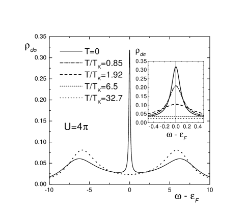
FIG. 1.: Spectral density at the dot for given spin, $U=4\pi,$ $\varepsilon_{d}=-2\pi,$ $\varepsilon_{F}=0,$ and several temperatures. $\Delta=1$ is chosen as the unit of energy.

A particular situation is the case $\varepsilon_{eff}=\varepsilon_{F},$ at which $\rho_{d\sigma}(\omega)$ is symmetric around $\varepsilon_{F}$ and then $n_{d\sigma}=1/2.$ At this point, the perturbative result satisfies exactly Friedel’s sum rule.[17] Out of this point, for large $U$, the perturbative result should be improved as discussed later in this section. For the symmetric model $(\varepsilon_{eff}=\varepsilon_{F}),$ the spectral density coincides with that obtained using Quantum Monte Carlo with Maximum Entropy method within statistical errors if $U/\Delta\lesssim 1.25\pi\simeq 3.93.$[18] For $U/\Delta\simeq 7.6,$ the difference between both results is $\sim 10\%.$ In Fig. 1 we show the spectral density in the symmetric case for $U/\Delta=4\pi.$ Although this ratio is beyond the validity of the perturbation theory, the result is in qualitative agreement with the corresponding result obtained using Wilson’s Renormalization Group (WRG),[19] The central (or Kondo) peak is broader in perturbation theory. However, if the Kondo temperature is defined as half width at half maximum $(T_{K}\simeq 0.10\Delta),$ the temperature dependence of the Kondo peak for $T<2T_{K}$ agrees within $20\%$ with WRG results. The temperature dependence of the rest of $\rho_{d\sigma}$ is very small.

As $\varepsilon_{eff}$ increases from the symmetric situation $\varepsilon_{eff}=\varepsilon_{F},$ the Kondo peak is slightly shifted to higher energies, but $\rho_{d\sigma}(\varepsilon_{F})$ remains high. However, for $U>5\Delta$, the perturbative result shifts to the opposite direction, leading to a violation of Friedel’s sum rule. This shortcoming can be cured using an interpolative solution for the self-energy:[13, 14, 15]

$$\Sigma_{\sigma}(\omega,T)=\frac{n_{d\overline{\sigma}}(1-n_{d\overline{\sigma}})\Sigma_{\sigma}^{(2)}}{n_{d\overline{\sigma}}^{0}(1-n_{d\overline{\sigma}}^{0})-[(1-n_{d\overline{\sigma}})U+\varepsilon_{d}^{V}-\varepsilon_{eff}^{0}]U^{-2}\Sigma_{\sigma}^{(2)}},$$ (24)

where $n_{d\sigma}^{0}=-\int f(\omega)\mathop{\rm Im}G_{d\sigma}^{0}(\omega)d\omega/\pi$ is the impurity occupation corresponding to the unperturbed impurity spectral density, and $\varepsilon_{d}^{V}=\varepsilon_{eff}-Un_{d\overline{\sigma}}$ is the effective impurity level for $U=0$ (see Eqs. (18) and (19)), which depends on the applied gate voltage $V_{g}$. This self energy leads to the exact $G_{d\sigma}(\omega)$ not only for $U=0$, but also for a decoupled dot ($\Delta=0$), and reproduces the leading term for $\omega\rightarrow\infty$. The effective unperturbed impurity level $\varepsilon_{eff}^{0}$ can be calculated selfconsistently at arbitrary temperatures imposing the condition $n_{d\sigma}^{0}=n_{d\sigma}$ [13, 14]. Unless otherwise stated, the results presented here are obtained following this approach. For $T=0$, the results can be improved further determining $\varepsilon_{eff}^{0}$ by imposing Friedel’s sum rule, as done by Kajueter and Kotliar to solve the impurity problem in the dynamical mean-field approach.[15] We call $\Sigma_{KK}$ the self energy obtained in this way.

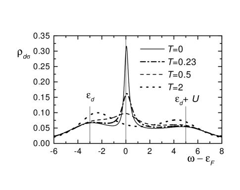
FIG. 2.:

In Fig. 2 we show the spectral density for $U=8\Delta$ in an asymmetric case with $\varepsilon_{d}-\varepsilon_{F}=-3\Delta$. The spectral density shows the characteristic charge fluctuation peaks near $\varepsilon_{d}$ and $\varepsilon_{d}+U,$ and the Kondo peak near $\varepsilon_{F}$. The slave-boson mean-field theory [5] cannot reproduce the charge fluctuation peaks and brings an incomplete description of the spectral density. For the symmetric case $\varepsilon_{d}-\varepsilon_{F}=-4\Delta$, the Kondo temperature defined as half-width at half-maximum of the Kondo peak is $T_{K}\simeq 0.23\Delta$.[20] In a scale of $T_{K}$, for increasing temperatures, the Kondo peak is rapidly suppressed, while the charge fluctuation peaks remain and absorb the spectral weight of the Kondo peak. For $T\sim T_{K}$, the density of states at the Fermi level $\rho_{d\sigma}(\varepsilon_{F})$ is reduced to approximately half its value at $T=0$.

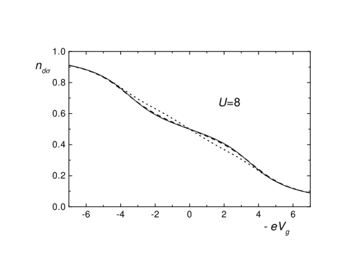
FIG. 3.: Dashed line: dot occupation for a given spin as a function of gate voltage for $U=8$, and $T=0$. Dotted line: corresponding result obtained from the phase shift at the Fermi level using Friedel’s sum rule. [17] Full line: result using $\Sigma_{KK}$ (imposing Friedel’s sum rule). The zero of $V_{g}$ is set at the point where $\varepsilon_{eff}=\varepsilon_{F},$ $n_{d\sigma}=1/2.$

In Fig. 3 we compare the resulting $n_{d\sigma}$ at $T=0$, with that obtained from the phase shift [17] for the largest $U$ (worst case) considered in this work ($U/\Delta=8$). We see that the deviations are small and concentrated near but out of the symmetric case. Note that the result using $\Sigma_{KK}$ (in which Friedel’s sum rule is imposed) is very similar to that obtained imposing $n_{d\sigma}^{0}=n_{d\sigma}$. In turn, this result agrees very well with exact calculations using the Bethe ansatz.[13]

IV Results for the conductance

From Eqs. (8), (9), (13), (14), (17), (18), (19), and (23), one can see that for given $U$ and $t^{\prime}\left(\text{or }t_{i}^{\prime}\right)\ll t,$ the conductance for the embedded and side dots depend on two parameters: $\Delta$ and $\varepsilon_{d}-eV_{g}.$ Furthermore, independently of the approximation used for the spectral density, both conductances are related shifting $V_{g}$ (or $\varepsilon_{d}$) and rescaling $\Delta:$

$$G_{e}(\Delta,V_{g}^{\prime})=\frac{4(t_{1}^{\prime}t_{-1}^{\prime})^{2}}{[(t_{1}^{\prime})^{2}+(t_{-1}^{\prime})^{2}]^{2}}\left[\frac{2e^{2}}{h}-G_{s}(\Delta,V_{g})\right],$$ (25)

with

$\displaystyle V_{g}^{\prime}=V_{g}+\left[(t_{1}^{\prime})^{2}+(t_{-1}^{\prime})^{2}\right]\frac{\varepsilon_{F}}{2t^{2}e}.$

Thus, it is sufficient to calculate one of the conductances.

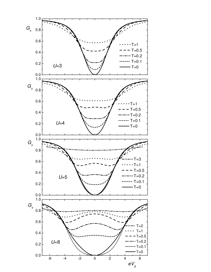
FIG. 4.: Conductance for the side dot in units of $2e^{2}/h$ as a function of gate voltage for several values of $U$ and $T$ indicated inside each figure. The bottom curve with thiner full line was obtained using $\Sigma_{KK}$.

In Fig. 4 we represent $G_{s}$ for several values of $U$ and $T.$ The unit of energy is set as $\Delta=1,$ the conductance is expressed in units of $2e^{2}/h$ and the zero of the gate voltage is set at the symmetric Anderson model ($eV_{g0}=\varepsilon_{d}+U/2=0$ for the side dot). For $T=0$ we have also included the result imposing Friedel’s sum rule,[15] (using $\Sigma_{KK}$) which gives a slightly smaller value of $G_{s}$ and allows to estimate the error at finite $T$. This error is due to the effect on $\rho_{d\sigma}(\varepsilon_{F})$ in the real part of $\Sigma(\varepsilon_{F})$ for the asymmetric Anderson model. The imaginary part is always zero as it should be for a Fermi liquid. For $U=8$, the difference in $G_{s}$ at $T=0$ between both interpolative methods attains its maximum value $\sim 0.07\times 2e^{2}/h$ near $eV_{g}-eV_{g0}=\pm 2.5$. For $U=5$, the maximum deviations are of the order of 2%, and for smaller $U$ they are negligible. Note that the difference between both approaches is much smaller in integral properties, like $n_{d\sigma}$ (see Fig. 3). As a consequence $G_{s}$ obtained using Eq. (16) (instead of Eq. (13)) is practically the same in both approaches. Using $\Sigma_{KK}$, of course Eq. (13) and Eq. (16) give identical results.

The conductance for $T=0$ and $U\geq 5$ are qualitatively similar to the corresponding result of Ref. 6. As the temperature is increased, $G_{s}$ near $V_{g}=0$ rapidly increases. This is expected from the temperature dependence of the Kondo peak, presented in the previous section. For $U\geq 5$, at temperatures of the order of the Kondo temperature $(T_{K}\simeq 0.45$ for $U=5$ and $T_{K}\simeq 0.23$ for $U=8$ defined as half width at half maximum of the Kondo spectral peak$),$ or slightly smaller, the conductance shows two minima. For $T>T_{K}$, the resulting structure is qualitatively what one expects for $t^{\prime}\rightarrow 0,$ in which only the Coulomb blockade peaks at $\varepsilon_{d}$ and $\varepsilon_{d}+U$ are important at finite temperatures. However, the peaks are displaced towards zero, particularly for small $U$ and $T$. For $U=5$ and $T>T_{K}$, the interpolative scheme and the ordinary second order perturbative result (using $\Sigma_{\sigma}=\Sigma_{\sigma}^{(2)}$ and with selfconsistency in $n_{d\sigma}$ only) are practically identical. At smaller temperatures, the ordinary treatment exaggerates the structure with two minima. Instead, the comparison with the results using $\Sigma_{KK}$ at $T=0$ and $U=8$, suggest that the interpolative treatment with $n_{d\sigma}=n_{d\sigma}^{0}$ inhibits somewhat this structure for large $U.$

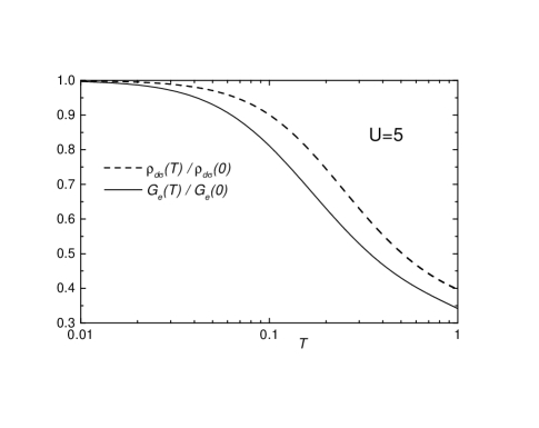
FIG. 5.: Temperature dependence of the conductance for the embedded dot and the density of states at the Fermi level for the symmetric Anderson model and $U=5\Delta.$

As $U$ is decreased, the structure with two minima weakens. For $U=3\Delta$ the Anderson model is near the intermediate valence regime, since the Kondo regime requires $U\gg\Delta.$ While the spectral density displays only one peak, without marked shoulders for $U=3,$ plateaus reminiscent to the transition to the Coulomb blockade regime are still present in the conductance for $0.2\leq T\leq 0.5$. In Fig. 5 we show the temperature dependence of the density of states at $\varepsilon_{F}$ and the conductance of the embedded dot for $V_{g}=0$ and $U=5.$ The shape of both quantities in a logarithmic temperature scale is similar to the experimentally observed conductance.[3] In our case the linear behavior with $\log T$ extends over less than an order of magnitude: from $T\sim 0.13$ to $\sim 0.5$ for $\rho_{d\sigma}(\varepsilon_{F})$ and from $\sim 0.1$ to $0.3$ for $G_{e}.$ This corresponds to values lower or of the order of $T_{K}.$

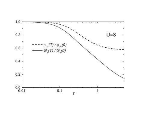
FIG. 6.: Same as Fig. 6 for $U=3\Delta.$

In Fig. 6, we show the same temperature dependence for $U=3.$ In this case, the half width at half maximum of the spectral density in the symmetric case is $0.73.$ In comparison with Fig. 5, the behavior of $\rho_{d\sigma}(\varepsilon_{F})$ and $G_{e}$ vs. $T$ is qualitatively different. $\rho_{d\sigma}(\varepsilon_{F})\sim\log T$ for $0.2\lesssim T\lesssim 0.6.$ In contrast, except for a very small curvature upwards, $G_{e}$ is linear in $\log T$ for $0.16\lesssim T\lesssim 2.$ A quadratic fit of all points with temperatures an integer times 0.01 in this interval gives $G_{e}h/(2e^{2})=0.4295-0.2112\log(T$ /$\Delta)+0.0050[\log(T$ /$\Delta)]^{2}$, with a mean square deviation $6\times 10^{-5}$.

V Summary and discussion

We have calculated the conductance for a quantum dot embedded in a quantum wire or side coupled to it as a function of gate voltage and temperature.. We have considered moderate values of $U$ which have not been studied before. For these values of $U,$ the perturbative method used is quite accurate. For small coupling of the dot to the wire, the conductance is determined by an integral of the density of states at the dot times the derivative of the Fermi function. As the temperature is increased, for $U\geq 4\Delta$ we find that the conductance as a function of the gate voltage changes from a typical shape with one extremum dominated by the Kondo peak in the spectral density, to another with two extrema, corresponding to the Coulomb blockade regime. To our knowledge, this crossover has not been reported previously.

For $U=3\Delta,$ we find that the conductance can be described as linear in $\log T$ as a very good approximation over more than an order of magnitude in $T.$ This behavior is rather unexpected and difficult to explain in simple terms, since different energy scales in the problem are of the same magnitude.

VI Acknowledgments

One of us (A.A.A.) wants to thank V. Zlatić and E. Anda for useful discussions. The authors are partially supported by CONICET. This work was sponsored by PICT 03-03833 from ANPCyT and PIP 4952/96 from CONICET.

REFERENCES

- [1] D. Goldhaber-Gordon, H. Shtrikman, D. Mahalu, D. Abusch-Magder, U. Meirav, and M. A. Kastner, Nature 391, 156 (1998).
- [2] S. M. Cronenwet, T. H. Oosterkamp, and L. P. Kouwenhoven, Science 281, 540 (1998).
- [3] D. Goldhaber-Gordon, J. Göres, M. A. Kastner, H. Shtrikman, D. Mahalu, and U. Meirav, Phys. Rev. Lett. 81, 5225 (1998).
- [4] B. R. Bulka and P. Stefanski, Phys. Rev. Lett. 86, 5128 (2001).
- [5] K. Kang, S. Y. Cho, J. J. Kim, and S. C. Shin, Phys. Rev. B 63, 113304 (2001).
- [6] M. E. Torio, K. Hallberg, A. H. Ceccatto, and C. R. Proetto, cond-mat/0108167.
- [7] A. C. Hewson, in The Kondo Problem to Heavy Fermions (Cambridge, University Press, 1993).
- [8] R. Franco, M.S. Figueira, and M.E. Foglio, cond-mat/0109037.
- [9] V. Ferrari, G. Chiappe, E. V. Anda, and M. A. Davidovich, Phys. Rev. Lett. 82, 5088 (1999).
- [10] K. Yosida and K. Yamada, Prog. Theor. Phys. Suppl. 46, 244 (1970); Prog. Theor. Phys. 53, 1286 (1975); K. Yamada, ibid 53, 970 (1975).
- [11] B. Horvatić, D. Šokčević, and V. Zlatić, Phys. Rev. B 36, 675 (1987).
- [12] M. Salomaa, Solid State Comm. 38, 815 (1981); ibid 39, 1105 (1981).
- [13] J. Ferrer, A. Martín-Rodero, and F. Flores, Phys. Rev. B 36, 6149 (1987)
- [14] A. Levy-Yeyati, A. Martín-Rodero, and F. Flores, Phys. Rev. Lett. 71, 2991 (1993).
- [15] H. Kajueter and G. Kotliar, Phys. Rev. Lett. 77, 131 (1996).
- [16] Y. Meir and N. S. Wingreen, Phys. Rev. Lett. 68, 2512 (1992).
- [17] D. C. Langreht, Phys. Rev. 150, 516 (1966).
- [18] R. N. Silver, J. E. Gubernatis, D. S. Sivia, and M. Jarrell, Phys. Rev. Lett. 65, 496 (1990).
- [19] T. A. Costi, A. C. Hewson, and V. Zlatić, J. Phys. 6, 2519 (1994).
- [20] The expression is valid only for very small .