NRCPS-HE-01-30

NTUA-9/01

Abstract

We perform Monte Carlo simulations of a three-dimensional spin system with a Hamiltonian which contains only four-spin interaction term. This system describes random surfaces with extrinsic curvature - gonihedric action. We study the anisotropic model when the coupling constants $\beta_{S}$ for the space-like plaquettes and $\beta_{T}$ for the transverse-like plaquettes are different. In the two limits $\beta_{S}=0$ and $\beta_{T}=0$ the system has been solved exactly and the main interest is to see what happens when we move away from these points towards the isotropic point, where we recover the original model. We find that the phase transition is of first order for $\beta_{T}=\beta_{S}\approx 0.25,$ while away from this point it becomes weaker and eventually turns to a crossover. The conclusion which can be drown from this result is that the exact solution at the point $\beta_{S}=0$ in terms of 2d-Ising model should be considered as a good zero order approximation in the description of the system also at the isotropic point $\beta_{S}=\beta_{T}$ and clearly confirms the earlier findings that at the isotropic point the original model shows a first order phase transition.

1 Introduction

In this article we shall consider a model of two-dimensional random surfaces embedded into a Euclidean lattice $Z^{3},$ where a closed surface is associated with a collection of plaquettes. The surfaces may have self-intersections in the form of four plaquettes intersecting on a link. Various models of random surfaces built out of plaquettes have been considered in the literature [1]. The gas of random surfaces defined in [2] corresponds to the partition function with Boltzmann weights proportional to the total number of plaquettes. In this article we shall consider the so-called gonihedric model with extrinsic curvature action [3, 4]. The gonihedric model of random surfaces corresponds to a statistical system with weights proportional to the total number of non-flat edges $n_{2}$ of the surface [3]. The weights associated with self-intersections are proportional to $kn_{4}$ where $n_{4}$ is the number of edges with four intersecting plaquettes, and $k$ is the self-intersection coupling constant [3, 4]. The partition function is a sum over two-dimensional surfaces of the type described above, embedded in a three-dimensional lattice:

$$Z(\beta)=\sum_{\{surfaces~{}M\}}e^{-\beta~{}\epsilon(M)},$$ (1)

where $\epsilon(M)=n_{2}+4kn_{4}$ is the energy of the surface $M$.

In three dimensions the equivalent spin Hamiltonian is equal to [4]

$$H_{gonihedric}^{3d}=-2k\sum_{\vec{r},\vec{\alpha}}\sigma_{\vec{r}}\sigma_{\vec{r}+\vec{\alpha}}+\frac{k}{2}\sum_{\vec{r},\vec{\alpha},\vec{\beta}}\sigma_{\vec{r}}\sigma_{\vec{r}+\vec{\alpha}+\vec{\beta}}-\frac{1-k}{2}\sum_{\vec{r},\vec{\alpha},\vec{\beta}}\sigma_{\vec{r}}\sigma_{\vec{r}+\vec{\alpha}}\sigma_{\vec{r}+\vec{\alpha}+\vec{\beta}}\sigma_{\vec{r}+\vec{\beta}},$$ (2)

and it is an alternative model to the $3D$ Ising system [2]

$$H_{Ising}^{3d}=-\sum_{\vec{r},\vec{\alpha}}\sigma_{\vec{r}}\sigma_{\vec{r}+\vec{\alpha}}.$$

The degeneracy of the vacuum state depends on self-intersection coupling constant $k$ [5]. If $k\neq 0$, the degeneracy of the vacuum state is equal to $3\cdot 2^{N}$ for the lattice of size $N^{3},$ while it equals $2^{3N}$ when $k=0$. The last case is a sort of supersymmetric point in the space of gonihedric Hamiltonians [5]

$$H_{gonihedric}^{k=0}=-\frac{1}{2}\sum_{\vec{r},\vec{\alpha},\vec{\beta}}\sigma_{\vec{r}}\sigma_{\vec{r}+\vec{\alpha}}\sigma_{\vec{r}+\vec{\alpha}+\vec{\beta}}\sigma_{\vec{r}+\vec{\beta}}.$$ (3)

This enhanced symmetry allows the construction of the dual Hamiltonian which has the form [5]

$$H^{k=0}_{dual}=-\sum_{\xi}\left[R^{\chi}(\xi)\cdot R^{\chi}(\xi+\chi)+R^{\eta}(\xi)\cdot R^{\eta}(\xi+\eta)+R^{\varsigma}(\xi)\cdot R^{\varsigma}(\xi+\varsigma)\right],$$ (4)

where $\chi$, $\eta$ and $\varsigma$ are unit vectors in the orthogonal directions of the dual lattice and $R^{\chi}$, $R^{\eta}$ and $R^{\varsigma}$ are one-dimensional irreducible representations of the group $Z_{2}\times Z_{2}$.

To study statistical and scaling properties of the system one can directly simulate surfaces by gluing together plaquettes with the corresponding weight $exp(-\beta(n_{2}+4kn_{4}))$ or (much easier) to study the equivalent spin system (2). The first Monte Carlo simulations [6, 7, 8, 9] demonstrate (see Figure 1) that the gonihedric system with intersection coupling constant greater than $k_{c}\approx 0.5$ (including $k=1),$ undergoes a second order phase transition at $\beta_{c}\approx 0.44$ and that the critical indices are different from those of the 3D Ising model. Thus they are in different classes of universality. On the contrary, the system shows a first order phase transition for $k<k_{c},$ including the “supersymmetric” point $k=0$.

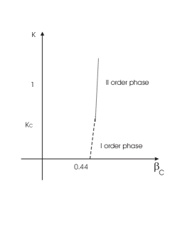
Figure 1: Phase diagram for different values of intersection coupling constant $k$.

Essential progress in our understanding of the physical behavior of the system has been achieved by means of the transfer matrix approach [5, 10]. The corresponding transfer matrix can be constructed for all values of the intersection coupling constant $k$ [11] and describes the propagation of the closed loops in the time direction. In this article we shall consider only the $k=0$ case. The corresponding transfer matrix has the form [5]

$$K(Q_{1},Q_{2})=\exp\{-\beta~{}[k(Q_{1})+2l(Q_{1}\bigtriangleup Q_{2})+k(Q_{2})]~{}\},$$ (5)

where $Q_{1}$ and $Q_{2}$ are closed polygon-loops on a two-dimensional lattice, $k(Q)$ is the curvature and $l(Q)$ is the length of the polygon-loop $Q$ . This transfer matrix describes the propagation of the initial loop $Q_{1}$ to the final loop $Q_{2}$ and corresponds exactly to the Hamiltonian (3),(4). Thus in order to study the critical behavior of the $k=0$ system (3),(4), (5) one should find the spectrum of the transfer matrix (5). Generally speaking all three dimensional problems of statistical mechanics are extremely complicated and in our case the exact solution still remains out of reach. However the breakthrough comes from the exact solution of a closed system when the transfer matrix depends only on the symmetric difference of initial and final loops $Q_{1}\bigtriangleup Q_{2}$ [10, 11]

$$\tilde{K}(Q_{1},Q_{2})=\exp\{-2\beta l(Q_{1}\bigtriangleup Q_{2})~{}\}.$$ (6)

The spectrum of the last system has been evaluated analytically in terms of correlation functions of the 2D Ising model. This is a nontrivial example of exactly solvable system in three dimensions. In particular the largest eigenvalue $\Lambda_{0}$ is exactly equal to the partition function of the 2d Ising model and the free energy of our 3d system is therefore equal to the free energy of the 2d Ising model. This result nicely explains why the critical temperature of the three-dimensional gonihedric system is so close to the critical temperature of the two-dimensional Ising model $2\beta_{c}=\frac{1}{2}ln(1+\sqrt{2})\approx 0.44$. The next to the largest eigenvalue $\Lambda_{1}$ of the 3d system (6) coincides with internal energy $u(\beta)$ of the two-dimensional Ising model

$${\Lambda_{1}\over\Lambda_{0}}~{}=~{}\langle\sigma_{\vec{r}}~{}\sigma_{\vec{r}+\hat{1}}\rangle~{}=~{}-u(\beta)$$ (7)

and the correlation length $\xi(\beta),$ defined through the ratio of eigenvalues $\Lambda_{1}/\Lambda_{0},$ is equal to:

$$\xi(\beta)={1\over-ln(\Lambda_{1}/\Lambda_{0})}={1\over-ln(-u(\beta))}.$$

If the internal energy $u(\beta)$ approaches $1,$ the correlation length tends to infinity and signals a second order phase transition in the system. But the internal energy of the 2d-Ising model drastically increases at the critical point $2\beta_{c}=\frac{1}{2}ln(1+\sqrt{2})$ without reaching the value 1 ! Thus, in three dimensions, we have the extraordinary situation that the specific heat has the logarithmic singularity of the 2d-Ising model, but the correlation length remains finite. The conclusion is that the system undergoes a weak first order phase transition rather than a second order phase transition. The Hamiltonian which corresponds to the transfer matrix (6) has been found in [11] and is equal to

$$\tilde{H}_{Q_{1}\bigtriangleup Q_{2}}=\sum_{E_{x},E_{y}}\sigma\sigma\sigma\sigma,$$ (8)

where a summation is only over $vertical$ plaquettes, the interactions take place only on the vertical planes $E_{x}$ and $E_{y}$ and the “horizontal” interactions have been switched off.

The above consideration poses the following interesting question: let us consider the system

$$H_{anisot}=\beta_{S}\sum_{E_{z}}\sigma\sigma\sigma\sigma+\beta_{T}\sum_{E_{x},E_{y}}\sigma\sigma\sigma\sigma,$$ (9)

which has anisotropic coupling constants for vertical and horizontal plaquettes. We have seen that when $\beta_{S}=0$ the system reduces to the system (6),(8) and as we just explained it has been solved in [10, 11]. When $\beta_{T}=0$ it factors into identical two dimensional plane systems solved in [5] and it is always in the disordered phase. Finally when $\beta_{S}=\beta_{T}$ we arrive at our original $k=0$ system (3),(4),(5). Thus we know the behavior of the system at both $\beta_{S}=0$ and $\beta_{T}=0$, but we still don’t know the analytical solution at the isotropic point $\beta_{S}=\beta_{T}$. The understanding of the phase structure of the anisotropic system (9) on $(\beta_{S},\beta_{T})$ plane by means of Monte Carlo simulations can drastically clarify the situation. Indeed, the important question to which we would like to find an answer is whether or not there is any dramatic changes in the behavior of the system when we move out of solvable point $\beta_{S}=0$ to the isotropic point $\beta_{S}=\beta_{T},$ where a first order phase transition has been observed in [7, 9]. Our Monte Carlo simulations show that there are no changes in the behavior of the system as it moves from $\beta_{S}=0$ to the isotropic point $\beta_{S}=\beta_{T}$. The conclusion which can be drawn from this result is that the exact solution at the point $\beta_{S}=0$ in terms of 2d-Ising model should be considered as a good zero order approximation in the description of the system also at the isotropic point $\beta_{S}=\beta_{T}$ if one consider a perturbation with the coupling constant $\beta_{S}/\beta_{T}$. This should be checked by further analytical consideration.

2 The lattice model

Thus the lattice action (9) may be written in the form

$$S\equiv\beta_{S}\sum P_{xy}+\beta_{T}\sum(P_{xz}+P_{yz}),$$

$$P_{xy}(\vec{r})\equiv 1-\sigma(\vec{r})\sigma(\vec{r}+\hat{x})\sigma(\vec{r}+\hat{x}+\hat{y})\sigma(\vec{r}+\hat{y}),$$

$$P_{xz}(\vec{r})\equiv 1-\sigma(\vec{r})\sigma(\vec{r}+\hat{x})\sigma(\vec{r}+\hat{x}+\hat{z})\sigma(\vec{r}+\hat{z}),$$

$$P_{yz}(\vec{r})\equiv 1-\sigma(\vec{r})\sigma(\vec{r}+\hat{y})\sigma(\vec{r}+\hat{y}+\hat{z})\sigma(\vec{r}+\hat{z}).$$

Our goal is to find the phase diagram in the extended $\beta_{S}-\beta_{T}$ plane. For that we shall calculate in the sequel the mean values of the action $S,$ the space-like plaquette $P_{S}\equiv P_{xy}$ and the transverse-like plaquette $P_{T}\equiv\frac{P_{xz}+P_{yz}}{2}.$ These quantities serve as order parameters which help us identify the various phases.

A first attempt towards the determination of the phase diagram is through the mean field approximation. One considers the free energy in the mean field approximation, which (up to additive constants) is given by the expression:

$$F(x)=-(\beta_{S}+2\beta_{T})[u^{\prime}(x)]^{4}-u(x)+xu^{\prime}(x).$$

The function $u(x)$ is defined through the relation

$$\exp[u(x)]\equiv e^{x}+e^{-x}=2\cosh(x)\rightarrow u(x)=\log(2)+\log[\cosh(x)]\rightarrow u^{\prime}(x)=\tanh(x).$$

We observe that $F(x)$ depends on the combination $B\equiv\beta_{S}+2\beta_{T}.$ The free energy has always a local minimum at $x=0.$ For small $B$ this is also the global minimum. As $B$ increases, a second minimum shows up, which eventually wins and becomes the global minimum at $B=0.688.$ Thus the phase transition line is given by:

$$\beta_{T}=\frac{0.688-\beta_{S}}{2}.$$

More accurately it is the segment of this line which corresponds to positive values of $\beta_{S}$ and $\beta_{T}.$ For $\beta_{S}=0$ we predict a critical value 0.344 for $\beta_{T},$ while as $\beta_{S}$ increases the critical value decreases and finally becomes zero at $\beta_{S}=0.688.$

For the first set of measurements we have fixed $\beta_{S}$ to several values, let $\beta_{T}$ run and found the hysteresis loops which have been formed. The results of these measurements are displayed in figure 2. The subfigures correspond to the lattice volumes $6^{3},8^{3},10^{3}$ and $12^{3}$ respectively. The line segments indicate the extents of the hysteresis loops. We have proceeded with steps of 0.005 for $\beta_{T}$ and performed 200 iterations at each point. We have used plain Metropolis Monte Carlo as a simulation technique. The phase transition line tends towards the horizontal axis for large $\beta_{S}.$ It is not clear from such measurements what happens for $\beta_{S}\rightarrow\infty,$ that is, whether the phase transition line meets the horizontal axis or it ends at some point. However, it is known analytically about the $\beta_{T}=0$ case that no phase transition should show up. Conceivably the transition weakens and eventually becomes a crossover before it meets the axis.

From the phase diagrams we may infer that the isotropic model will have a phase transition at $\beta_{S}=\beta_{T}\approx 0.25.$ This value is approximately the point where the $\beta_{S}=\beta_{T}$ line meets the phase transition line.

Figure 2: Phase diagram for $\beta_{S}$ fixed at several values for $6^{3},8^{3},10^{3},12^{3}$ lattices.

After this first overview of the phase structure we will study some of its characteristics in more detail. To this end we have performed long runs, sticking to a particular point of the parameter space, that is specific values for $\beta_{S}$ and $\beta_{T}$ and performing about three million iterations. When the parameters are near a first order phase transition we expect to see the eventual two-state signals. As a by-product of this procedure, the critical points may be determined with much greater accuracy than the one provided by the hysteresis loop method. We have found that, if we fix $\beta_{S},$ the critical $\beta_{T}$ increases slightly with the volume, while for the isotropic model the volume dependence is very small.

We now proceed with the presentation of the behaviour of the system in the immediate vicinity of the phase transition. The computer time evolution will be depicted for $8^{3}$ lattices. We concentrated on three values of $\beta_{S},$ namely 0.00, 0.20 and 0.60 and tried several values of $\beta_{T}$ near the critical point.

In figure 3 we show the time evolution of the transverse-like plaquette for a $8^{3}$ lattice for $\beta_{S}=0.00$ and various values of $\beta_{T}$ around 0.34. The system fluctuates violently and, as $\beta_{T}$ increases, it gradually spends its time more and more in the low $P_{T}$ region. This behaviour provides evidence that the transition is of higher order.

In figure 4 we present the time evolution of the transverse plaquette for $\beta_{S}=0.20$ in the phase transition region, that is for $\beta_{T}$ around 0.26. We may clearly see the oscillation of the mean values between the two metastable states and the gradually increasing importance of the “low $P_{T}$” metastable phase with respect to the “high $P_{T}$” one as $\beta_{T}$ increases. More precisely, the system starts by spending most of its “time” in the state with large $P_{T},$ but it gradually starts visiting also the state with the small $P_{T},$ until at some point it spends most of its time in the small $P_{T},$ as shown in the last subfigure. A very similar behaviour shows up for $\beta_{S}=0.30.$

For $\beta_{S}=0.60$ the picture is strongly reminiscent of the $\beta_{S}=0.00$ case. Figure 5 shows relatively long runs for several values of $\beta_{T}$ around 0.11. The system performs large fluctuations again and its mean value drifts toward small values of $P_{T}$ as $\beta_{T}$ increases.

It appears that the phase transition is first order around the value $\beta_{S}\simeq 0.25,$ it remains strong for $\beta_{S}$ not very different from this value, but it weakens substantially for too small or too large values.

Figure 3: Time evolution of the transverse-like plaquette for a $8^{3}$ lattice at $\beta_{S}=0.000$ and $\beta_{T}=0.330,0.340,0.343,0.347.$

Figure 4: Time evolution of the transverse-like plaquette for a $8^{3}$ lattice at $\beta_{S}=0.200$ and $\beta_{T}=0.256,0.258,0.260,0.262.$

Figure 5: Time evolution of the transverse-like plaquette for a $8^{3}$ lattice at $\beta_{S}=0.600$ and $\beta_{T}=0.105,0.110,0.115,0.120.$

Finally, in figure 6 we present the time evolution of the plaquette for the isotropic model on a $8^{3}$ lattice. For $\beta$ around 0.24 we observe the phase transition and we may see the two metastable states. The fluctuations of the system between the two metastable states are very similar to the ones of the anisotropic model with $\beta=0.20.$ It appears that the phase transition is quite strong here, in agreement with previously obtained results.

Figure 6: Long runs for the isotropic model at $\beta_{g}=0.236,0.238,0.240$ and $0.242.$

The final statement about the order of the phase transitions should come from a study of the volume dependence of the susceptibilities and the Binder cumulants. However, as one increases the volume, the system sticks to either of the metastable states and one cannot really observe the oscillation between the two states in a reasonable time. The only exception occurs for rather small lattice volumes. We have already presented the results for $8^{3}$ lattices, but it is difficult to observe something similar for larger volumes. However, one can easily see that if the susceptibility varies linearly with the volume (which is the sign of a first order transition), the gap between the two metastable states should be volume independent. Thus, we may get an idea about the order of the phase transitions by studying the volume dependence of the gap. If it is volume independent, we have a first order transition. If it decreases with the volume, there is a weaker phase transition (second or higher order). We find out that the gap does not actually depend on the volume. Figure 7 shows the results for $\beta_{S}=0.20.$ Thus it appears that this phase transition is of first order. The same picture also appears for $\beta_{S}=0.30.$ This means that there are first order phase transitions in a region around $0.25.$ For $\beta_{S}$ away from this region one cannot really define a gap (compare figure 5). It is clear, however, that the phase transition is weak in this regime.

Figure 7: The gap versus the volume.

3 Acknowledgements

One of the authors G.S. was supported in part by the EEC Grant HPRN CT 199900161. G.K. acknowledges the support from EEC Grant no. ERBFMRX CT 970122 and he would like to thank P.Dimopoulos for useful discussions.

References

-
[1]
D.Weingarten. Nucl.Phys.B210 (1982) 229
A.Maritan and C.Omero. Phys.Lett. B109 (1982) 51
T.Sterling and J.Greensite. Phys.Lett. B121 (1983) 345
B.Durhuus,J.Fröhlich and T.Jonsson. Nucl.Phys.B225 (1983) 183
J.Ambjørn,B.Durhuus,J.Fröhlich and T.Jonsson. Nucl.Phys.B290 (1987) 480
T.Hofsäss and H.Kleinert. Phys.Lett. A102 (1984) 420
M.Karowski and H.J.Thun. Phys.Rev.Lett. 54 (1985) 2556
F.David. Europhys.Lett. 9 (1989) 575 - [2] F.J. Wegner, J. Math. Phys.12 (1971) 2259
-
[3]
G.K. Savvidy and K.G. Savvidy,
Int. J. Mod. Phys. A8 (1993) 3993
R.V. Ambartzumian, G.K. Savvidy , K.G. Savvidy and G.S. Sukiasian. Phys. Lett. B275 (1992) 99
G.K. Savvidy and K.G. Savvidy. Mod.Phys.Lett. A8 (1993) 2963
B.Durhuus and T.Jonsson. Phys.Lett. B297 (1992) 271 -
[4]
G.K.Savvidy and F.J.Wegner. Nucl.Phys.B413(1994)605
G.K. Savvidy and K.G. Savvidy. Phys.Lett. B324 (1994) 72
R. Pietig and F.J. Wegner. Nucl.Phys. B466 (1996) 513 -
[5]
G.K. Savvidy and K.G. Savvidy. Phys.Lett. B337 (1994) 333;
Mod.Phys.Lett. A11 (1996) 1379
G.K. Savvidy, K.G. Savvidy and P.G. Savvidy. Phys.Lett. A221 (1996) 233
G. K. Savvidy, K. G. Savvidy and F. J. Wegner. Nucl.Phys. B443 (1995) 565 - [6] G.K.Bathas, E.Floratos, G.K.Savvidy and K.G.Savvidy. Mod.Phys.Lett. A10 (1995) 2695
-
[7]
D.Johnston and R.K.P.C.Malmini, Phys.Lett. B378 (1996) 87,
D.Johnston and R.K.P.C.Malmini, Nucl.Phys.Proc.Suppl.53:773-776,1997,
M.Baig, D.Espriu, D.Johnston and R.K.P.C.Malmini,
J.Phys. A30 (1997) 407; J.Phys. A30 (1997) 7695,
A.Lipowski and D.Johnston, cond-mat/9812098. -
[8]
G.Koutsoumbas et.al. Phys.Lett. B410 (1997)
241
-
[9]
A.Cappi, P.Colangelo, G.Gonnella
and A.Maritan, Nucl. Phys. B370 (1992) 659
G.Gonnella, S.Lise and A.Maritan, Europhys. Lett. 32 (1995) 735
E.N.M.Cirillo and G.Gonnella. J.Phys.A: Math.Gen.28 (1995) 867
E.N.M.Cirillo, G.Gonnella and A.Pelizzola, Phys.Rev. E55, R17 (1997)
E.N.M.Cirillo, G.Gonnella D.Johnston and A.Pelizzola, Phys.Lett. A226, 59 (1997)
E.N.M.Cirillo, G.Gonnella and A.Pelizzola, Nucl.Phys. (Proc.Suppl.) 63, 622 (1998)
-
[10]
T.Jonsson and G.K.Savvidy. Phys.Lett.B449 (1999) 254;
Nucl.Phys. B575 (2000) 661-672, hep-th/9907031 - [11] G.K.Savvidy. JHEP 0009 (2000) 044