Uniaxial and biaxial soft deformations of nematic elastomers

Abstract

We give a geometric interpretation of the soft elastic deformation modes of nematic elastomers, with explicit examples, for both uniaxial and biaxial nematic order. We show the importance of body rotations in this non-classical elasticity and how the invariance under rotations of the reference and target states gives soft elasticity (the Golubovic and Lubensky theorem). The role of rotations makes the Polar Decomposition Theorem vital for decomposing general deformations into body rotations and symmetric strains. The role of the square roots of tensors is discussed in this context and that of finding explicit forms for soft deformations (the approach of Olmsted).

I Introduction

Nematic elastomers display three unique and related phenomena not found in conventional elasticity - large spontaneous deformations, very large optical-mechanical response and soft elasticity. The last, shape change with little or no energy cost, is the subject of this paper. We give a geometric interpretation of the soft modes described using fractional powers of tensors. We then discuss the soft modes of biaxial nematic elastomers. Since in contrast to conventional elastic solids, rotations play an essential role in the elasticity of nematic rubber, we conclude by discussing the related questions of breaking finite strains into symmetric shears and rotations, the Polar Decomposition Theorem for tensors, and the nature of square roots of tensors.

Nematic elastomers have an internal, orientational degree of freedom in addition to those of ordinary elastic bodies. The anisotropy of molecular orientation induces shape anisotropy in the polymers that make up the elastomer. The switching on and off of this molecular shape anisotropy, either by temperature changeKüpfer and Finkelmann (1994) or by illuminationFinkelmann et al. (2001), causes large ($\approx 400\%$) mechanical shape changes.

Rotation of this anisotropy, by imposed mechanical strains, is the extreme opto-mechanical effect that is observed. When accompanied by subsidiary shears and contractions which accommodate the changes of molecular distributions, the cost of the originally imposed strain is rendered to zero . This is what we call soft elasticityWarner et al. (1994).

II Softness in linear continua

One can explore the related ideas of anisotropy, rotation and soft elasticity initially for small deformations and rotations, that is within the linear continuum theory of a uniaxial body with a mobile director ${\bf{n}}$ that characterises the anisotropy directionde Gennes (1980). The free energy density, $F$, is:

$$F = \textstyle\frac{1}{2}\tilde{B}({\rm Tr}[\underline{\underline{{{\tilde{\varepsilon}}}}}])^{2}+\textstyle\frac{1}{2}\kappa\ {\rm Tr}[\underline{\underline{{{\tilde{\varepsilon}}}}}]({\bf n}\cdot\underline{\underline{{{\varepsilon}}}}\cdot{\bf n})\ +\textstyle\frac{1}{2}\mu_{0}({\bf n}\cdot\underline{\underline{{{\varepsilon}}}}\cdot{\bf n})^{2}$$

$$+\textstyle\frac{1}{2}\mu_{1}[{\bf n}\times\underline{\underline{{{\varepsilon}}}}\times{\bf n}]^{2}+\textstyle\frac{1}{2}\mu_{2}([{\bf n}\times\underline{\underline{{{\varepsilon}}}}]\cdot{\bf n})^{2}$$

$$+\textstyle\frac{1}{2}D_{1}[(\bm{\Omega}-\bm{\omega})\times{\bf n}]^{2}+\textstyle\frac{1}{2}D_{2}\,{\bf n}\cdot\underline{\underline{{{\varepsilon}}}}\cdot[(\bm{\Omega}-\bm{\omega})\times{\bf n}],$$

where $\underline{\underline{{{\varepsilon}}}}=\underline{\underline{{{\tilde{\varepsilon}}}}}-\frac{1}{3}{\rm Tr}[\underline{\underline{{{\tilde{\varepsilon}}}}}]\ \underline{\underline{{{\delta}}}}$ is the traceless part of the linear symmetric strain $\tilde{\varepsilon}_{ij}=\frac{1}{2}(\partial_{j}u_{i}+\partial_{i}u_{j})$, and ${\bf\Omega}=\frac{1}{2}{\rm curl}\ {\bf u}$ is the antisymmetric part (the body rotation), ${\bf u}$ being the displacement field.

The latter terms are those of the relative rotation $(\bm{\Omega}-\bm{\omega})\times{\bf n}$ coupling: for small rotations, the director variation corresponds to a rotation $\bm{\omega}={\bf n}\times\delta{\bf n}_{\bm{\omega}}$ or $\delta{\rm\bf n}_{\bm{\omega}}=\bm{\omega}\times{\rm\bf n}$, see fig. 1. Similarly, a small rotation $\bm{\Omega}$ of the matrix causes a vector ${\rm\bf v}$ in the body to suffer the change $\delta{\rm\bf v}_{\bm{\Omega}}=\bm{\Omega}\times{\rm\bf v}$.

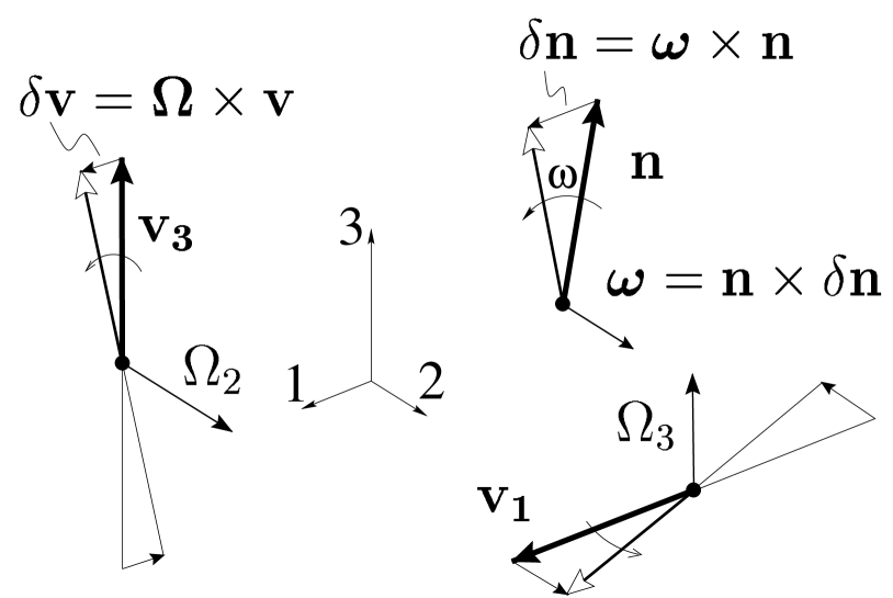
Figure 1: Rotation of ${\bf{n}}$ about an axis $\bm{\omega}$, and body rotations $\bm{\Omega}$ rotating vectors ${\rm\bf v}$. Only $\Omega_{2}$ and $\Omega_{1}$ (not shown) have any effect on vectors parallel to ${\bf{n}}$.

The net rotation of ${\bf{n}}$ with respect to the matrix inflicted by the relative rotation $\bm{\Omega}-\bm{\omega}$ of the matrix ($\bm{\Omega}$) relative to the changing director ($\bm{\omega}$) accordingly gives a relative change in ${\bf{n}}$ of:

$$\delta{\rm\bf n}=(\bm{\Omega}-\bm{\omega})\times{\bf{n}}\ .$$

The directors ${\bf{n}}$ and ${\bf{n}}_{0}$ before and after application of strain are not distinguished in the first terms of equation (II) for small director rotation, but clearly must be in the relative rotation coupling terms in $F$.

The tensor $\underline{\underline{{{\tilde{\varepsilon}}}}}$ is the strain before it has been made traceless, that is, it still has volume changes ${\rm Tr}\left(\underline{\underline{{{\tilde{\varepsilon}}}}}\right)$ in it. Since rubber is a soft material, its deformations are at constant volume and we neglect the first two terms in equation (II) since they involve volume change. The geometry of the remaining strains is vital and shown in fig. 2.

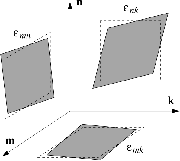
Figure 2: The elements of strain in a uniaxially anisotropic medium. Dashed lines show the undistorted state, whereas the strained elements are shown by shaded areas. They divide into stretches ${\varepsilon}_{nn}$ along ${\bf{n}}$, stretches ${\varepsilon}_{mm}$ and ${\varepsilon}_{kk}$ and distortions ${\varepsilon}_{mk}$ in the plane perpendicular to ${\bf{n}}$, and distortions ${\varepsilon}_{nm}$ and ${\varepsilon}_{nk}$ encompassing ${\bf{n}}$ and the perpendicular plane.

The de Gennes de Gennes (1980) relative rotation couplings are unique to nematic networks because they require an independent, rotational degree of freedom, i.e., the rotations $\bm{\omega}$ of the director n. Its motion in the medium is coupled to the body rotation ${\bm{\Omega}}$. Hence, the elastic energy unusually involves antisymmetric components of shear strain. In section VI, we accordingly show how to extract the rotational component from any finite shear. The first coupling, $D_{1}$, purely resists the rotation of the director relative to a rotating, undeformed matrix. The $D_{2}$ term couples ${\bf{n}}$ to the symmetric part of shear in the plane that involves ${\bf{n}}$ (e.g. $\varepsilon_{zx}$ if $n_{0}=n_{z}$ in equilibrium). These are the shears ${\varepsilon}_{nm}$ and ${\varepsilon}_{nk}$ in fig. 2. Since infinitesimal, incompressible symmetric shear is equivalent to stretch along one diagonal and compression along another, it is reasonable that prolate molecules will reduce the cost of distortion by rotating their ordering direction to being as much as possible along the elongation diagonal, depicted in fig. 3. Oblate elastomers rotate their director toward the compression diagonal to achieve the appropriate elastic accommodation. The spheroid represents the anisotropic shape distribution of the crosslinked polymers from which the network is composed.

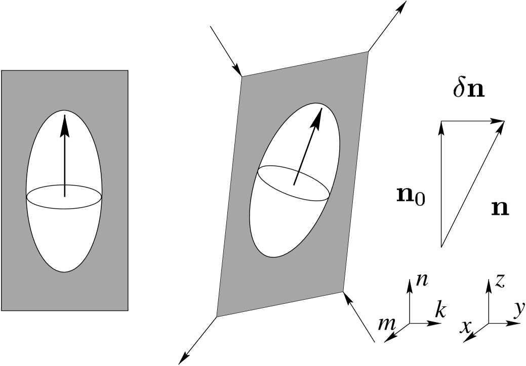
Figure 3: Symmetric shear induces director rotation toward the elongation diagonal. The respective elongations and compressions along the diagonals are shown. The chain shape distribution also rotates. When mechanical shape changes of a network accommodate the rotations of the chain distribution without distortions, such shape changes can take place at minimal energy cost.

A theorem of Golubovic and Lubensky (GL) Golubovic and Lubensky (1989) shows that on symmetry grounds any solid with an internal degree of freedom which is also capable of reaching an isotropic reference state must be invariant under the double set of rotations of both the reference and target states when considering elastic deformations. This has the remarkable consequence that some elastic deformations must be soft. This was discovered independently and in a superficially different form when studying at finite deformations the elastic response of nematic elastomers Warner et al. (1994). We sketch how this can be understood for elastomers in order to explain the complex soft modes we shall later discuss.

An effective shear modulus arises for an imposed elastic strain, when the nematic director is free to evolve optimally. The elastic modulus $\mu_{2}$ is reduced; by the symmetry argument it must vanish to give no overall energy cost. If the local rotational component $\bm{\Omega}$ of the deformation of the elastic matrix and the rotation of the director are coaxial, i.e. $\bm{\Omega}$ and $\bm{\omega}$ are parallel and uniform, the argument is simple. Minimising the relative-rotation part of the energy density (II), $\frac{1}{2}D_{1}[(\bm{\Omega}-\bm{\omega})\times{\bf n}]^{2}+\frac{1}{2}D_{2}\,{\bf n}\cdot{\underline{\underline{{{\varepsilon}}}}}\cdot[(\bm{\Omega}-\bm{\omega})\times{\bf n}]$, one obtains the optimal relative rotation for a given shear strain $\underline{\underline{{{{\varepsilon}}}}}$:

$$[(\bm{\Omega}-\bm{\omega})\times{\bf n}]=-\frac{D_{2}}{2D_{1}}({\bf n}\cdot\underline{\underline{{{{\varepsilon}}}}})\ {\rm or}\ \ (\bm{\Omega}-\bm{\omega})=-\frac{D_{2}}{2D_{1}}[{\bf n}\cdot\underline{\underline{{{{\varepsilon}}}}}\times{\bf n}]\ .$$ (2)

We now substitute this back into the energy density and obtain for the rotation-strain terms:

$$\textstyle\frac{1}{2}D_{1}[(\bm{\Omega}-\bm{\omega})\times{\bf n}]^{2}+\textstyle\frac{1}{2}D_{2}\,{\bf n}\cdot{\underline{\underline{{{\varepsilon}}}}}\cdot[(\bm{\Omega}-\bm{\omega})\times{\bf n}]$$ (3)

$$=-\frac{D_{2}^{2}}{8D_{1}}[{\bf n}\cdot\underline{\underline{{{{\varepsilon}}}}}\times{\bf n}]^{2}\equiv-\frac{D_{2}^{2}}{8D_{1}}\left({{\varepsilon}_{xz}}^{2}+{{\varepsilon}_{yz}}^{2}\right)\;.$$

The last expression is written in the specific coordinate frame where the initial director ${\bf n}_{0}$ is parallel to $z$-axis. We can now unite this expression with the rest of the elastic energy density, equation (II) and thus obtain the effective rubber-elastic energy which depends only on strains; the director does not appear. For instance, in the specific coordinates of fig. 2:

$$F = \textstyle\frac{1}{2}\mu_{0}\,{{\varepsilon}_{zz}}^{2}+\textstyle\frac{1}{2}\mu_{1}({{\varepsilon}_{xx}}^{2}+2{{\varepsilon}_{xy}}^{2}+{{\varepsilon}_{yy}}^{2})$$ (4)

$$+\textstyle\frac{1}{2}\left(\mu_{2}-\frac{D_{2}^{2}}{4D_{1}}\right)({{\varepsilon}_{xz}}^{2}+{{\varepsilon}_{yz}}^{2})\;.$$

The modulus $\mu_{2}$ is renormalised to $\mu_{2}-{D_{2}^{2}}/{(4D_{1})}$ which by the GL theorem must be zero, thus establishing a relation between the constants $\mu_{2}$, $D_{1}$, and $D_{2}$. The molecular model, required below for finite deformations, produces linear continuum limiting values which also give:

$$\mu_{2}^{\rm R}=\mu_{2}-\frac{D_{2}^{2}}{4D_{1}}\rightarrow 0\;.$$ (5)

Olmsted Olmsted (1994) first proposed this continuum mechanism behind the Golubovic–Lubensky theorem: shape depends on the orientation of an internal (nematic) degree of freedom, the rotation of which causes a natural shape change at zero cost for suitable solids. A general discussion of the GL argument and its extension to semi-softness and thresholds to rotation is given in Warner (1999). The experimental evidence for mechanically soft distortions is also discussed there.

One can picture the continuous rotation generating mechanical distortion at low energy cost, see Fig. 3. The natural long axis of the body, as defined by the principal axis of molecular shape, rotates in an attempt to follow the apparent extension axis. To the extent that macroscopic shape change can thus be imitated, there is no real accompanying distortion of polymer shape. We quantify this picture below when considering non-linear elasticity theory.

III Finite soft elasticity

A simple extension of classical rubber elasticity theory to nematic elastomers gives for the free energy density:

$$F=\textstyle\frac{1}{2}\mu{\rm Tr}\left(\underline{\underline{{{\ell}}}}_{\rm 0}\cdot\underline{\underline{{{\lambda}}}}^{\rm T}\cdot\underline{\underline{{{\ell}}}}^{-1}\cdot\underline{\underline{{{\lambda}}}}\right)$$ (6)

where $\mu$ is the rubber elastic shear modulus in the isotropic phase and $\lambda_{ij}=\partial R_{i}/\partial R_{0j}$ is the homogeneous deformation (gradient). If we take $\underline{\underline{{{\lambda}}}}$ to be $\underline{\underline{{{\lambda}}}}=\underline{\underline{{{\delta}}}}+\underline{\underline{{{u}}}}$, then the symmetric part of $\underline{\underline{{{u}}}}$ is identical to $\underline{\underline{{{\tilde{\varepsilon}}}}}$ of (II) in the infinitesimal limit.

The chains are no longer characterised by spherical Gaussian distributions as in the classical case, but in general by anisotropic distributions. Thus the effective step length tensors $\underline{\underline{{{\ell}}}}_{\rm 0}$ initially and $\underline{\underline{{{\ell}}}}$ currently after a distortion $\underline{\underline{{{\lambda}}}}$ are prolate (or oblate) spheroids defining the second moments that characterise the Gaussian distribution of chain spans ${\rm\bf R}$ in the the network, that is $\left<R_{i}R_{j}\right>=\frac{1}{3}\ell_{ij}L$ where $L$ is the arc length of a chain. Thus a measure of the mean size of a chain is $\underline{\underline{{{\ell}}}}^{1/2}$ where we shall soon define the roots of tensors more carefully. The tensor $\underline{\underline{{{\ell}}}}$ has one principal value $\ell_{\parallel}$ along ${\rm\bf n}$ and $\ell_{\bot}$ perpendicular to ${\rm\bf n}$; thus

$$\underline{\underline{{{\ell}}}}=\left(\begin{smallmatrix}\ell_{\bot}&0&0\\ 0&\ell_{\bot}&0\\ 0&0&\ell_{\parallel}\end{smallmatrix}\right)=\ell_{\bot}\left(\begin{smallmatrix}1&0&0\\ 0&1&0\\ 0&0&r\end{smallmatrix}\right),$$

where $r=\ell_{\parallel}/\ell_{\bot}$. The extracted $\ell_{\bot}$ factor from $\underline{\underline{{{\ell}}}}_{0}$ cancels with the $1/\ell_{\bot}$ factor extracted from $\underline{\underline{{{\ell}}}}^{-1}$ when both tensors appear together in the Trace formula (6) and we can henceforth just consider the $\underline{\underline{{{\ell}}}}$ tensors in their reduced form that simply depends on the intrinsic anisotropy $r$. Anisotropy varies between $r=1.1\rightarrow 60$. In this model of rubber elasticity the spontaneous elongation, $\lambda_{\rm m}$, on going from the isotropic to the nematic phase turns out to be $\lambda_{\rm m}=r^{\rm 1/3}$ and is thus a direct measure of $r$. Indeed spontaneous elongations in the range of $\lambda_{\rm m}\sim 1.03-4.00$ are observed.

Now distortions $\underline{\underline{{{\lambda}}}}$ are no longer small, but must continue to respect volume conservation, $\rm{Det}(\underline{\underline{{{\lambda}}}})=1$ in the non-linear regime. The directors ${\rm\bf n}_{\rm 0}$ and ${\rm\bf n}$, of the initial and current nematic states, may be greatly rotated from each other.

The remainder of this paper is concerned with explaining the character of the soft modes within finite elasticity theory and extending this picture to that of soft modes in biaxial nematic elastomers. We explore the role of rotations and the connections between the isolation of rotational components of strain at finite amplitude (the spherical decomposition theorem) and the relation of the roots of tensors to this picture.

IV Uniaxial softness

Consider the strain Olmsted (1994):

$$\underline{\underline{{{\lambda}}}}=\underline{\underline{{{\ell}}}}^{1/2}\cdot\underline{\underline{{{W}}}}_{\alpha}\cdot\underline{\underline{{{\ell}}}}^{-1/2}_{\rm 0}\;,$$ (7)

where $\underline{\underline{{{W}}}}_{\alpha}$ is an arbitrary rotation by an angle $\alpha$. There are two continuous degrees of freedom describing the rotation connecting ${\bf{n}}$ and ${\bf{n}}_{0}$ and three degrees of freedom for the rotation $\underline{\underline{{{W}}}}_{\alpha}$. Hence, the strain $\underline{\underline{{{\lambda}}}}$ is described by five continuous degrees of freedom and thus represents a large set of deformations.

If we insert such a strain into the Trace formula (6), as well as its transpose $\underline{\underline{{{\lambda}}}}^{\sf T}$ (equivalent to $\underline{\underline{{{\ell}}}}_{\rm 0}^{-1/2}\cdot\underline{\underline{{{W}}}}_{\alpha}^{\sf T}\cdot\underline{\underline{{{\ell}}}}^{1/2}$ since the $\underline{\underline{{{\ell}}}}$ are symmetric) we obtain:

$$F_{\rm el} = \textstyle\frac{1}{2}\mu{\rm Tr}\left(\underline{\underline{{{\ell}}}}_{\rm 0}\cdot\underline{\underline{{{\ell}}}}_{\rm 0}^{-1/2}\cdot\underline{\underline{{{W}}}}^{\sf T}_{\alpha}\cdot\underline{\underline{{{\ell}}}}^{1/2}\cdot\underline{\underline{{{\ell}}}}^{-1}\cdot\underline{\underline{{{\ell}}}}^{1/2}\cdot\underline{\underline{{{W}}}}_{\alpha}\cdot\underline{\underline{{{\ell}}}}^{-1/2}_{\rm 0}\right)$$ (8)

$$\equiv \textstyle\frac{1}{2}\mu{\rm Tr}\left(\underline{\underline{{{\delta}}}}\right)=\frac{3}{2}\mu\;.$$

Cancelling the middle section, $\underline{\underline{{{\ell}}}}^{1/2}\cdot\underline{\underline{{{\ell}}}}^{-1}\cdot\underline{\underline{{{\ell}}}}^{1/2}=\underline{\underline{{{\delta}}}}$, allows the $\underline{\underline{{{W}}}}$-terms to meet and gives $\underline{\underline{{{W}}}}^{\sf T}\cdot\underline{\underline{{{W}}}}=\underline{\underline{{{\delta}}}}$. Likewise disposing of the $\underline{\underline{{{\ell}}}}_{\rm 0}$ terms, one obtains the final expression $F_{\rm el}=\frac{3}{2}\mu$. This is identical to the free energy of an undistorted network. The non-trivial set of distortions $\underline{\underline{{{\lambda}}}}$ of this particular form, equation (7), have not raised the energy of nematic elastomer. From the results $\rm{Det}(\underline{\underline{{{A}}}}\cdot\underline{\underline{{{B}}}})=\rm{Det}(\underline{\underline{{{A}}}})\rm{Det}(\underline{\underline{{{B}}}})$, $\rm{Det}(\underline{\underline{{{A}}}}^{-1})=(\rm{Det}(\underline{\underline{{{A}}}}))^{-1}$ and $\rm{Det}(\underline{\underline{{{W}}}})=1$ for all rotations $\underline{\underline{{{W}}}}$, one can see that $\rm{Det}(\underline{\underline{{{\lambda}}}})=\rm{Det}(\underline{\underline{{{\ell}}}}^{1/2}\cdot\underline{\underline{{{W}}}}_{\alpha}\cdot\underline{\underline{{{\ell}}}}^{-1/2}_{\rm 0})=1$, that is these soft modes are volume-preserving.

We saw pictorially in fig. 3 that, on applying a stretch perpendicular to the initial director, rotation of the chain distribution is accommodated by the very elongation we have applied, together with a shear. Two remarkable consequences immediately follow from nematic elastomer response via rotation:

Impose an $x$-extension $\lambda_{xx}$. All the accompanying distortions must be in the plane of rotation, that is a transverse contraction $\lambda_{zz}$ and shears $\lambda_{xz}$ and $\lambda_{zx}$ accommodate the rotation of the distribution. No shears perpendicular to this plane, that is involving $y$-direction ($\lambda_{yy},\lambda_{yx},\dots$ etc.) are needed. For a classical isotropic elastomer $\lambda_{yy}=\lambda_{zz}=1/\sqrt{\lambda_{xx}}$ is demanded by incompressibility, whereas in soft elasticity there is no shrinkage in the $y$ direction ($\lambda_{yy}=1$) and the appropriate Poisson ratio is zero.

Fig. 4 shows the initial and final states of which the shear and partial rotation of fig. 3 is an intermediate step.

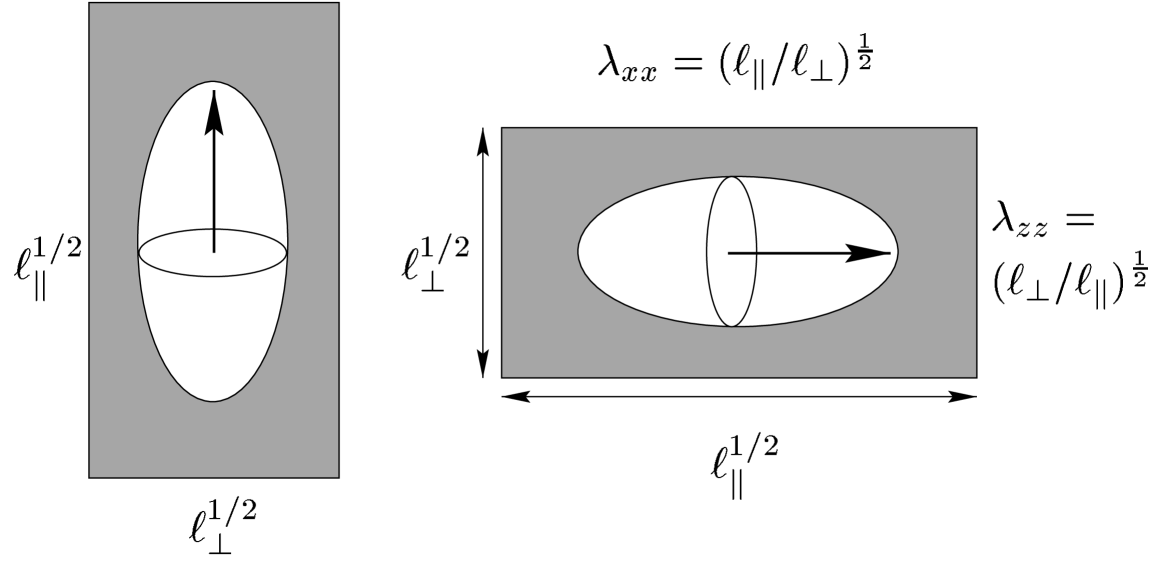
Figure 4: Chain shape distribution before and after rotations. The extent of soft extensions ($\lambda_{xx}$) perpendicular to the initial director is set by the anisotropy of the molecular shape distribution. The macroscopic dimensions are shown changing affinely with the distribution, for instance the $x$ dimension changing from $\sqrt{\ell_{\bot}}$ to $\sqrt{\ell_{\parallel}}$.

Softness must come to an end when the rotation is complete and the $z$ dimension has diminished in the proportion $\lambda_{zz}=\sqrt{\ell_{\bot}/\ell_{\parallel}}$ and the $x$ dimension extended in the proportion $\lambda_{xx}=\sqrt{\ell_{\parallel}/\ell_{\bot}}$. The original sizes $\sqrt{\ell_{\parallel}}$ and $\sqrt{\ell_{\bot}}$ have transformed to $\sqrt{\ell_{\bot}}$ and $\sqrt{\ell_{\parallel}}$ respectively. Thus softness would cease and director rotation be complete at $\lambda_{xx}=r^{1/2}\equiv\lambda_{\rm m}^{3/2}$. The strain $\lambda_{\rm m}=(\ell_{\parallel}/\ell_{\bot})^{1/3}$ is the spontaneous extension suffered on cooling to the nematic phase. Likewise one can imagine from an oblique form of figure 4 that if the initial director ${\bf{n}}_{0}$ (long axis of the shape ellipsoid) is not at $90^{\rm o}$ to the imposed strain, then rotation and softness is complete at a smaller $\lambda_{xx}<\lambda_{\rm m}$.

We give as a concrete example the set of soft distortions $\underline{\underline{{{\lambda}}}}_{\rm soft}=\underline{\underline{{{\ell}}}}^{1/2}_{\theta}\cdot\underline{\underline{{{\ell}}}}_{\rm 0}^{-1/2}$, simplified by the absence of the arbitrary rotation matrix $\underline{\underline{{{W}}}}_{\alpha}$. They are simply characterised (parametrically) by the angle $\theta$ by which $\underline{\underline{{{\ell}}}}_{\rm 0}$ is rotated to $\underline{\underline{{{\ell}}}}_{\theta}$, that is by which ${\bf{n}}_{\rm 0}$ is rotated to ${\bf{n}}$. Putting in the dyadic forms for $\underline{\underline{{{\ell}}}}_{\rm 0}^{-1/2}$ and $\underline{\underline{{{\ell}}}}^{1/2}_{\theta}$ into $\underline{\underline{{{\lambda}}}}_{\rm soft}$ gives:

$$\underline{\underline{{{\lambda}}}}_{\rm soft} = (\underline{\underline{{{\delta}}}}+(\sqrt{r}-1){\bf{n}}{\bf{n}}^{\sf T})\cdot(\underline{\underline{{{\delta}}}}+(\frac{1}{\sqrt{r}}-1){\bf{n}}_{\rm 0}{\bf{n}}_{0}^{\sf T})$$ (9)

$$= \underline{\underline{{{\delta}}}}+(1/\sqrt{r}-1){\bf{n}}_{\rm 0}{\bf{n}}_{0}^{\sf T}+(\sqrt{r}-1){\bf{n}}{\bf{n}}^{\sf T}$$

$$+({\bf{n}}.{\bf{n}}_{0})(2-\sqrt{r}-1/\sqrt{r}){\bf{n}}{\bf{n}}_{0}^{\sf T}\;.$$

If ${\bf{n}}_{\rm 0}$ is along $\hat{{\rm\bf z}}$ and is rotated by $\theta$ toward $\hat{{\rm\bf x}}$, it becomes ${\bf{n}}=\hat{{\rm\bf z}}\cos\theta+\hat{{\rm\bf x}}\sin\theta$. We can write down a particular representation of $\underline{\underline{{{\lambda}}}}_{\rm soft}$ (using the notation $s\equiv\sin\theta$ and $c\equiv\cos\theta$):

$$\underline{\underline{{{\lambda}}}}_{\rm soft} = \hat{{\rm\bf z}}\hat{{\rm\bf z}}^{\sf T}(1-(1-\frac{1}{\sqrt{r}})s^{2})+\hat{{\rm\bf x}}\hat{{\rm\bf x}}^{\sf T}(1+(\sqrt{r}-1)s^{2})$$ (10)

$$+\hat{{\rm\bf y}}\hat{{\rm\bf y}}^{\sf T}+\hat{{\rm\bf x}}\hat{{\rm\bf z}}^{\sf T}(1-\frac{1}{\sqrt{r}})sc+\hat{{\rm\bf z}}\hat{{\rm\bf x}}^{\sf T}(\sqrt{r}-1)sc$$

$$\equiv \begin{pmatrix}1+(\sqrt{r}-1)s^{2}&0&(1-1/\sqrt{r})sc\cr 0&1&0\cr(\sqrt{r}-1)sc&0&1-(1-1/\sqrt{r})s^{2}\end{pmatrix}\;.$$

The soft modes are neither simple nor pure shear, but a mixture of the two. Accordingly, the soft modes have an element of body rotation in addition to elongations, compressions and pure shears. The importance of body rotations is discussed before and after (2). The degree of body rotation is given in section VI. Note that the extensional and compressional strains $(\lambda_{xx}-1)$ and $(1-\lambda_{zz})$ are both proportional to $\sin^{2}\theta$. Thus the infinitesimal strains $u_{zz}$ and $u_{xx}$, at small rotations $\theta$, are proportional to $\theta^{2}$. By contrast $\lambda_{xz}$ and $\lambda_{zx}$ are proportional to $\sin\theta\,\cos\theta$ and hence the infinitesimals $u_{xz}$ and $u_{zx}$ are proportional to $\theta$ – a lower order than $u_{xx}$ and $u_{zz}$. There is no relaxation along $y$, perpendicular to the plane of rotation ${\rm\bf n}$, that is $\lambda_{yy}=1$. Also note that in the isotropic limit ($r=1$) this particular strain $\underline{\underline{{{\lambda}}}}_{\rm soft}=\underline{\underline{{{\delta}}}}$ while the general soft deformation (7) reduces to the null strain, $\underline{\underline{{{W}}}}_{\alpha}$, a simple body rotation. Both are the trivial cases evidently preserving the elastic energy at its minimum. The soft modes become non-trivial deformations when the material becomes a nematic elastomer.

The soft modes start at no strain, $\underline{\underline{{{\lambda}}}}=\underline{\underline{{{\delta}}}}$, and as the director $\theta$ rotates from 0 to $\pi/2$, they eventually end at

$$\underline{\underline{{{\lambda}}}}=\left(\begin{smallmatrix}\sqrt{r}&0&0\\ 0&1&0\\ 0&0&1/\sqrt{r}\end{smallmatrix}\right),$$

that is an extension $\lambda_{xx}=\sqrt{r}$ and a transverse contraction $\lambda_{zz}=1/\sqrt{r}$.

The director rotation is taken up by a shape change so that there is no entropically expensive deformation of the chain distribution as when a conventional elastomer deforms. The shape tensor’s anisotropy $r=\ell_{\parallel}/\ell_{\bot}$ characterises the ratio of the mean square size along the director to that perpendicular to the director. The square root of this ratio, $\sqrt{r}$, gives the characteristic ratio of average dimensions of chains in the network. During a soft deformation, the solid must change shape such that the rotating ellipsoid $\underline{\underline{{{\ell}}}}^{1/2}$, characterising the physical dimensions of the distribution of chains, is accommodated without distortion. The ellipsoid is ${{\rm\bf R}}\cdot\underline{\underline{{{\ell}}}}^{-1}\cdot{{\rm\bf R}}=1$, or in a principal frame, $x^{2}/r+z^{2}=1$, that is in section the ellipse has semi-major axes of $\sqrt{r}$ and $1$. Fig. 5 illustrates soft deformations of a nematic elastomer with chains of anisotropy $r=2$. The distortions are parameterised by the director rotation, $\theta$, which ranges between $0$ and $\pi/2$. The chain shape tensor, $\underline{\underline{{{\ell}}}}^{1/2}$, rotates without distortion, just fitting into the solid into which it embedded.

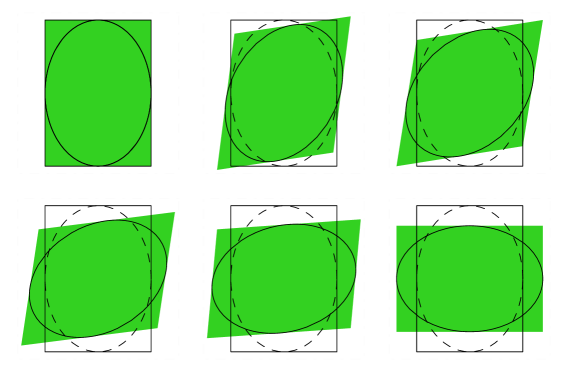
Figure 5: Soft deformations of a nematic elastomer with anisotropy $r=2$. The deformations correspond to director rotations of $\theta=0$, $\pi/6$, $\pi/4$, $\pi/3$, $5\pi/12$ and $\pi/2$ which parametrically generate the distortions as discussed above. Note that the prolate spheroid characterising the distribution of chains, embedded in the distorting solid (shaded and shown in section), when rotated by $\theta$ can be accommodated without distortion. The reference, undeformed body is shown in outline; the original distribution shown dashed.

The soft deformations of fig. 5 and equations (9) and (10) of the body are in general non-symmetric. Below we decompose these into pure shears plus rotations. One can think of $\underline{\underline{{{\lambda}}}}_{\rm soft}=\underline{\underline{{{\ell}}}}^{1/2}_{\theta}\cdot\underline{\underline{{{\ell}}}}_{\rm 0}^{-1/2}$ as converting the initial ellipsoid of fig. 5 to a sphere by the action of the inverse $\underline{\underline{{{\ell}}}}_{\rm 0}^{-1/2}$ and then recreating an ellipsoid at an angle $\theta$ with the action of $\underline{\underline{{{\ell}}}}^{1/2}_{\theta}$. This is precisely the scheme of deSimone and Dorfmann (2000); Lubensky et al. (2001) who consider an isotropic reference state (the intermediate created after the action of $\underline{\underline{{{\ell}}}}_{\rm 0}^{-1/2}$). We discuss this rotational invariance again below.

V Biaxial Softness

Biaxial nematic phases are rare. They have been found (Finkelmann et al Hessel and Finkelmann (1987); Leube and Finkelmann (1991)) in nematic polymers since one has more complex molecular structural possibilities. In principle such polymers could be used to make biaxially nematic elastomers. They would have rich mechanical properties.

The shape tensor of a biaxial polymer is

$$\underline{\underline{{{\ell}}}}=\left(\begin{smallmatrix}\ell_{1}&0&0\\ 0&\ell_{2}&0\\ 0&0&\ell_{\parallel}\end{smallmatrix}\right).$$

Now the step lengths in the two directions perpendicular to ${\bf{n}}$, $\ell_{1}$ and $\ell_{2}$, are distinguished. The tensor is reduced by taking out a factor of the mean perpendicular step length, $\ell_{\bot}=\textstyle\frac{1}{2}(\ell_{1}+\ell_{2})$, to give:

$$\underline{\underline{{{\ell}}}} = \left(\begin{smallmatrix}1+p/2&0&0\cr 0&1-p/2&0\cr 0&0&r\end{smallmatrix}\right)$$

$$\equiv r{\bf{n}}{\bf{n}}^{\sf T}+(1+\frac{p}{2}){\rm\bf m}{\rm\bf m}^{\sf T}+(1-\frac{p}{2}){\rm\bf k}{\rm\bf k}^{\sf T}$$

$$\equiv \underline{\underline{{{\delta}}}}+(r-1){\bf{n}}{\bf{n}}^{\sf T}+\frac{p}{2}{\rm\bf m}{\rm\bf m}^{\sf T}-\frac{p}{2}{\rm\bf k}{\rm\bf k}^{\sf T}$$

where the axes of the ellipsoid are ${\bf{n}}$, ${\rm\bf m}$ and ${\rm\bf k}$ (with the latter a third perpendicular axis given by ${\rm\bf k}={\bf{n}}\times{\rm\bf m}$), see fig. (6). The biaxiality is $p=2\frac{\ell_{1}-\ell_{2}}{\ell_{1}+\ell_{2}}=\frac{\ell_{1}-\ell_{2}}{\ell_{\bot}}$.

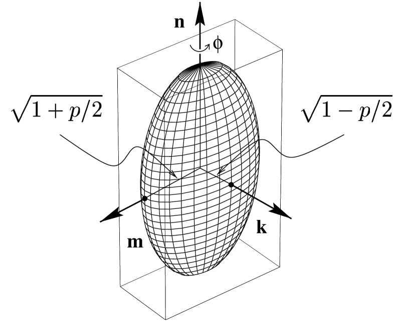
Figure 6: The shape ellipsoid for a biaxially nematic polymer. The section perpendicular to ${\bf{n}}$ is not circular, but has semi-axes of length $\sqrt{1\pm p/2}$. Rotations $\phi$ about ${\bf{n}}\equiv{\bf{n}}_{0}$ generate distortions in the $xy$ plane that softly accommodate the non-circular shape as it rotates.

With fixed ${\bf{n}}$, in the biaxial case one can rotate the anisotropic transverse section $mk$ of the square root of the shape tensor, $\underline{\underline{{{\ell}}}}^{1/2}$, and accommodate it without distortion by inducing shape changes in the $mk$ plane. These distortions are soft for exactly the same reasons as in the uniaxial case when ${\bf{n}}$ suffered rotations in the $nk$ or $nm$ planes, see figs. 5. Given that there are (now in the Lab. frame) $\lambda_{xy}$ soft modes as well as the $\lambda_{zx}$ and $\lambda_{zy}$ forms (which are now no longer equivalent modes), the order of softness has become very much greater.

V.1 Explicit examples of soft modes arising from biaxiality

The situation is exactly parallel to that of the soft shears (9) and (10). Now the soft modes are given by $\underline{\underline{{{\ell}}}}^{1/2}_{\phi}\underline{\underline{{{\ell}}}}^{-1/2}_{\rm 0}$ where $\phi$ is instead the angle of rotation about the principal director ${\bf{n}}$. The tensor $\underline{\underline{{{\ell}}}}_{\rm 0}^{1/2}$ is

$$\underline{\underline{{{\ell}}}}^{1/2}_{0}=\left(\begin{smallmatrix}\sqrt{1+p/2}&0&0\\ 0&\sqrt{1-p/2}&0\\ 0&0&\sqrt{r}\end{smallmatrix}\right),$$ (11)

which will then be rotated by $\phi$. By analogy with fig. 5, the anisotropy in the $xy$ part of the matrix which is to be rotated is $\sqrt{r_{\bot}}=\sqrt{\frac{1+p/2}{1-p/2}}\equiv\sqrt{\frac{\ell_{1}}{\ell_{2}}}$. This measures the anisotropy of actual (root mean square) chain dimensions in the plane perpendicular to the director. The resulting soft shears in the $xy$-plane arising from rotations $\phi$ about ${\bf z}={\bf n}_{0}$ are:

$$\underline{\underline{{{\lambda}}}}_{\rm biaxial}=\left(\begin{smallmatrix}1-(1-1/\sqrt{r_{\bot}})s^{2}_{\phi}&(1-\sqrt{r_{\bot}})s_{\phi}c_{\phi}&0\cr(1/\sqrt{r_{\bot}}-1)s_{\phi}c_{\phi}&1+(\sqrt{r_{\bot}}-1)s_{\phi}^{2}&0\cr 0&0&1\end{smallmatrix}\right)\;.$$ (12)

More complicated soft shears are possible if these shears are combined with those previously found in the uniaxial case. For example, in the uniaxial case, section (IV) above, subsequent rotation about ${\bf{n}}$ after the rotation of ${\bf{n}}$ itself had no effect since there was symmetry about ${\bf{n}}$. Now that this is lost, such rotations will reorient the perpendicular directors ${\rm\bf m}$ and ${\rm\bf k}$ and thereby induce additional soft shears.

V.2 General biaxial softness

If, however, the axis of rotation does not coincide with a principal axis as in the previous examples, we discover soft modes of lower symmetry, which only lead back to an undeformed body after the chain distribution has been rotated by $2\pi$. Consider as an example of reduced symmetry the situation when the chain distribution is rotated around a general axis in the $xy$ plane at an angle $\beta$ to the $x$ axis (fig. 7): a rotation of $\pi$ (fig. 8) transfers the director ${\bf n}$ (along the $z$-axis) into $-{\bf n}$, but the unit vectors ${\bf m}$ and ${\bf k}$ along the other two principal axes end up in a general position in the $xy$-plane. The same final position of the ellipsoid of chain distribution can be obtained by a rotation around the $z$-axis by an appropriate angle. The corresponding body deformation leaves all $z$-coordinates invariant, but transforms the the $xy$-coordinates as if they have suffered a body rotation of $2\beta$ about $z$.

If we were to choose the axis of rotation in an arbitrary way, we would not observe this feature of invariant $z$-components after a rotation of $\pi$. Only a full rotation of $2\pi$ would lead back into a state of higher symmetry, in this case, of course, the identity.

By rotating the ellipsoid of chain distribution, we create soft modes, which are closely related to the underlying symmetry, which is the crystal class of the biaxial ellipsoid, the dipyramidal orthorhombic class.

Comparing with equation (7), we see that so far we have set the rotation $\underline{\underline{{{W}}}}_{\alpha}$ to be the identity. If, however, we were to allow a general rotation, we would find an even larger set of deformations, in fact described by six degrees of freedom: the additional rotations $\underline{\underline{{{W}}}}_{\alpha}$ and the rotations connecting the principal frames of the initial and final ellipsoids each introduce three degrees of freedom.

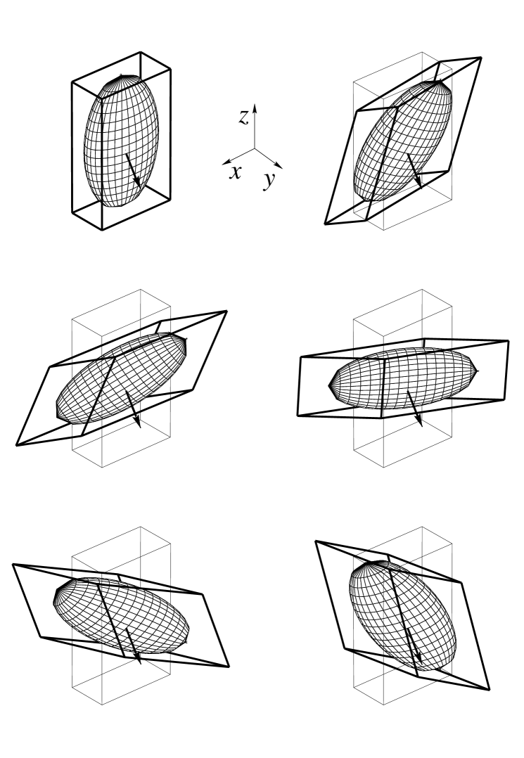
Figure 7: Rotation of the chain distribution around an axis (arrow) in the $xy$-plane at an angle of $\pi/3$ with the $x$-axis. The figure shows intermediate states of rotation at an angle of 0, $\pi$, $\frac{1}{6}\pi$,$\frac{1}{3}\pi$,$\frac{1}{2}\pi$,$\frac{2}{3}\pi$ and $\frac{5}{6}\pi$. Fig. (8) shows the final stage of a rotation by an angle of $\pi$. The fine outline shows the initial body shape, whereas the highlighted outline illustrates the body deformation as the the ellipsoid of the internal chain distribution rotates. Here, we have chosen $p=6/5$ and $r=200/45$, or, equivalently, the principal axes of the ellipsoid to be 6, 3 and 10 respectively.

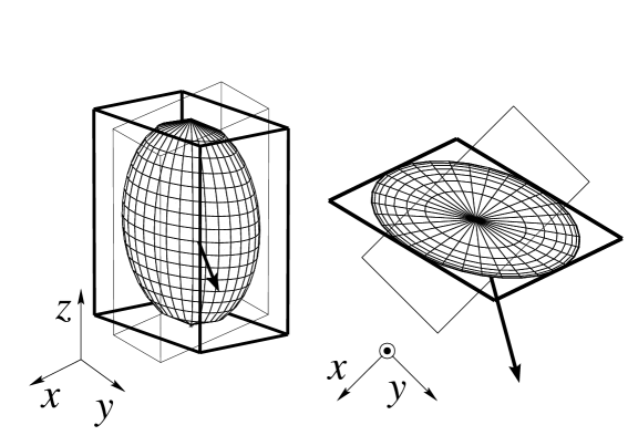
Figure 8: Rotation of the chain distribution by $\pi$ around an axis in the $xy$-plane at an angle of $\pi/3$ with the $x$-axis. The figure shows two views of the same situation: the final ellipsoid together with the outlines of the bodies which indicate the corresponding soft mode deformation. The outline of the deformed body is highlighted. The parameters are the same as in fig. (7).

VI Rotations, symmetric strains and the roots of tensors

We have seen in equations (II)–(4) yielding softness that rotations are vital to understanding soft elasticity. The cartoon of fig. 5 shows that soft shears are not symmetric and hence there must be a component of body rotation present. Here we explore the role of rotations in symmetry requirements. We then explicitly extract the rotational component from general distortions and from soft deformations in particular. The requirements for extracting the rotational components of the strain tensor are intimately related to finding the square roots of tensors which we discuss here since they are used in constructing soft deformations.

Any general matrix $\underline{\underline{{{M}}}}$ can be broken down into products $\underline{\underline{{{S}}}}\cdot\underline{\underline{{{O}}}}$ or $\underline{\underline{{{O}}}}\cdot\underline{\underline{{{S}}}}^{\prime}$ of symmetric matrices $\underline{\underline{{{S}}}}$ and $\underline{\underline{{{S}}}}^{\prime}$ and orthogonal matrices $\underline{\underline{{{O}}}}$ and $\underline{\underline{{{O}}}}^{\prime}$, which can be restricted to proper rotations. In effect, one has a pure shear preceded or followed by a body rotation (the Polar Decomposition Theorem Horn and Johnson (1991)).

Note that in the infinitesimal case, we have $\underline{\underline{{{S}}}}=\underline{\underline{{{1}}}}+\underline{\underline{{{\delta S}}}}$ and $\underline{\underline{{{O}}}}=\underline{\underline{{{1}}}}+\underline{\underline{{{\delta O}}}}$, hence $\underline{\underline{{{\delta S}}}}=\underline{\underline{{{\delta S}}}}^{\sf T}$ and $\underline{\underline{{{\delta O}}}}=-\underline{\underline{{{\delta O}}}}^{\sf T}$. Analogous statements hold for the matrices $\underline{\underline{{{S}}}}^{\prime}$ and $\underline{\underline{{{O}}}}^{\prime}$. This shows that the rotation matrices $\underline{\underline{{{O}}}}$ and $\underline{\underline{{{O}}}}^{\prime}$ are related to the antisymmetric part of the deformation in the infinitesimal limit.

Applied to the deformation $\underline{\underline{{{\lambda}}}}$, we write:

$$\underline{\underline{{{\lambda}}}}=\underline{\underline{{{\lambda}}}}^{\rm L}\cdot\underline{\underline{{{V}}}}\;\;\;\ {\rm or}\;\;\;\underline{\underline{{{U}}}}\cdot\underline{\underline{{{\lambda}}}}^{\rm R},$$ (13)

where the rotations are denoted by $\underline{\underline{{{V}}}}$ or $\underline{\underline{{{U}}}}$ depending upon whether they act on the reference or target spaces respectively of the deformation. The form of the accompanying symmetric deformations will depend on the order; they are denoted by $\underline{\underline{{{\lambda}}}}^{\rm R}$ and $\underline{\underline{{{\lambda}}}}^{\rm L}$ respectively and yield the Cauchy-Green tensors $\underline{\underline{{{C}}}}$ and $\underline{\underline{{{B}}}}$ respectively: $\underline{\underline{{{C}}}}=\underline{\underline{{{\lambda}}}}^{\sf T}\cdot\underline{\underline{{{\lambda}}}}$ and $\underline{\underline{{{B}}}}=\underline{\underline{{{\lambda}}}}\cdot\underline{\underline{{{\lambda}}}}^{\sf T}$.

We summarise classical elasticity theory to highlight the differences with nematic rubber elasticity. The deformation (gradient) is:

$$\lambda_{ij}=\partial R_{i}/\partial R_{0j}\;.$$ (14)

If the target space ($S_{T}$) deforms under rotations represented by the matrix $\underline{\underline{{{U}}}}$, as ${{\rm\bf R}}^{\prime}=\underline{\underline{{{U}}}}\cdot{{\rm\bf R}}$, and the reference space ($S_{R}$) deforms under rotations $\underline{\underline{{{V}}}}$ as ${{\rm\bf R}}_{0}^{\prime}=\underline{\underline{{{V}}}}\cdot{{\rm\bf R}}_{0}$, then the deformation tensor deforms as

$$\lambda^{\prime}_{ij} = U_{ik}\partial R_{k}/\partial R_{0l}V^{\rm\sf T}_{lj}$$ (15)

$$\underline{\underline{{{\lambda}}}}^{\prime} = \underline{\underline{{{U}}}}\cdot\underline{\underline{{{\lambda}}}}\cdot\underline{\underline{{{V}}}}^{\rm\sf T}\quad{\rm or}\quad\underline{\underline{{{\lambda}}}}=\underline{\underline{{{U}}}}^{\rm\sf T}\cdot\underline{\underline{{{\lambda}}}}^{\prime}\cdot\underline{\underline{{{V}}}}\;.$$ (16)

Thus $\underline{\underline{{{\lambda}}}}$ records the character of both the target and reference states, a property that will be essential in non-ideal nematic elastomers where an isotropic reference state cannot be reached. The connection with both spaces is quite different in character from that of the Cauchy tensors. Thus the combination

$$\underline{\underline{{{C}}}} = \underline{\underline{{{\lambda}}}}^{\rm\sf T}\cdot\underline{\underline{{{\lambda}}}}=\underline{\underline{{{V}}}}^{\rm\sf T}\cdot{\underline{\underline{{{\lambda}}}}^{\prime}}^{\sf T}\cdot\underline{\underline{{{U}}}}\cdot\underline{\underline{{{U}}}}^{\rm\sf T}\cdot\underline{\underline{{{\lambda}}}}^{\prime}\cdot\underline{\underline{{{V}}}}$$ (17)

$$= \underline{\underline{{{V}}}}^{\rm\sf T}\cdot{\underline{\underline{{{\lambda}}}}^{\prime}}^{\sf{T}}\cdot\underline{\underline{{{\lambda}}}}^{\prime}\cdot\underline{\underline{{{V}}}}=\underline{\underline{{{V}}}}^{\rm\sf T}\cdot\underline{\underline{{{C}}}}^{\prime}\cdot\underline{\underline{{{V}}}}$$

is manifestly invariant under body rotations $\underline{\underline{{{U}}}}$ of the final (target) space $S_{T}$ and transforms as a second rank tensor in $S_{R}$. Since isotropic systems are invariant to rotations $\underline{\underline{{{V}}}}$ of $S_{R}$, the system’s final energy must be invariant to rotations of $S_{R}$. Thus $F$ is a function of the rotational (in $S_{R}$) invariants of $\underline{\underline{{{C}}}}$ and is assured by the above of being invariant under rotations of $S_{T}$. As an example, the isotropic rubber elastic free energy, setting $\underline{\underline{{{\ell}}}}^{\rm 0}=\underline{\underline{{{\ell}}}}^{\rm-1}=\underline{\underline{{{\delta}}}}$ in equation (6) is

$$F = \textstyle\frac{1}{2}\mu{\rm Tr}\left(\underline{\underline{{{C}}}}\right)=\textstyle\frac{1}{2}\mu{\rm Tr}\left(\underline{\underline{{{V}}}}^{\rm\sf T}\cdot\underline{\underline{{{C}}}}^{\prime}\cdot\underline{\underline{{{V}}}}\right)$$ (18)

$$= \textstyle\frac{1}{2}\mu{\rm Tr}\left(\underline{\underline{{{C}}}}^{\prime}\cdot\underline{\underline{{{V}}}}\cdot\underline{\underline{{{V}}}}^{\rm\sf T}\right)=\textstyle\frac{1}{2}\mu{\rm Tr}\left(\underline{\underline{{{C}}}}^{\prime}\right)$$ (19)

(by cyclical properties of the trace). Likewise, $\underline{\underline{{{B}}}}=\underline{\underline{{{\lambda}}}}\cdot\underline{\underline{{{\lambda}}}}^{\rm\sf T}$, is invariant to rotations of the reference state and transforms like a second rank tensor in the target state.

Thus we see that “objectivity”, frame indifference, is built into classical elasticity theory from the outset. Nematic elastomers are much more subtle. In continuum theory we have seen that rotations and symmetric shears enter, both separately (through the de Gennes $D_{1}$ term) and coupled (through the $D_{2}$ term). In finite elasticity, we see in the Trace formula that the initial and final orientations of the solid and its directors enters via the tensors $\underline{\underline{{{\ell}}}}^{\rm 0}$ and $\underline{\underline{{{\ell}}}}^{\rm-1}$ and there are not combinations like $\underline{\underline{{{B}}}}$ and $\underline{\underline{{{C}}}}$ which eliminate rotations. For instance, inserting $\underline{\underline{{{U}}}}\cdot\underline{\underline{{{\lambda}}}}^{\rm R}$ into the trace result, one obtains:

$$F=\textstyle\frac{1}{2}\mu{\rm Tr}\left(\underline{\underline{{{\ell}}}}_{\rm 0}\cdot\underline{\underline{{{\lambda}}}}^{\rm R\;{\sf T}}\cdot[\underline{\underline{{{U}}}}^{\rm\sf T}\cdot\underline{\underline{{{\ell}}}}^{-1}\cdot\underline{\underline{{{U}}}}]\cdot\underline{\underline{{{\lambda}}}}^{\rm R}\right)$$ (20)

where the $[\dots]$ have been inserted to emphasise that a body rotation of $S_{T}$ effectively adds to the rotation of ${\bf{n}}$. That is, a new $\underline{\underline{{{\ell}}}}^{\prime}$ evolves: ${\underline{\underline{{{\ell}}}}^{\prime}}^{-1}=\underline{\underline{{{U}}}}^{\sf T}\underline{\underline{{{\ell}}}}^{-1}\underline{\underline{{{U}}}}$. (The additional rotation is not necessarily coaxial with that which took ${\bf{n}}_{\rm 0}$ to ${\bf{n}}$.) Not unexpectedly, we see the effect of $\underline{\underline{{{U}}}}$ compounded with the rotations implicit in $\underline{\underline{{{\ell}}}}^{-1}$ since they both live in the target space.

Other approaches have been taken deSimone and Dorfmann (2000); Lubensky et al. (2001) to soft elasticity which apparently circumvent the necessity to follow orientations in both spaces, and restore objectivity. One can measure all deformations $\underline{\underline{{{\lambda}}}}$ from an isotropic reference state, that is there is encoded into the $\underline{\underline{{{\lambda}}}}$ first a spontaneous deformation to current conditions of temperature, then a deformation imposed with respect to this intermediate state. Under these conditions the free energy must automatically be invariant under operations of $\underline{\underline{{{V}}}}$, since the reference state is isotropic and without a director ${\rm\bf n}_{\rm 0}$ to keep track of. Difficulties arise then when nematic elastomers are only semi-soft, that is, they do not deform entirely at constant free energy, because they do not have a high temperature isotropic reference state. However they do suffer director rotation, very low energy trajectories in $\underline{\underline{{{\lambda}}}}$ space and a lack of $\lambda_{yy}$ relaxation perpendicular to the plane of ${\rm\bf n}$’s rotation Verwey et al. (1996). In these cases, the complete cancellation rendering $\mu_{2}^{\rm R}=\mu_{2}-\frac{D_{2}^{2}}{4D_{1}}\rightarrow 0$ fails, but nevertheless deformations are qualitatively soft and one has to keep track of both directions ${\rm\bf n}_{\rm 0}$ and ${\rm\bf n}$ as strain evolves.

VI.1 Square roots of tensors and the Polar Decomposition Theorem

We quote the classical conditionsHorn and Johnson (1991) for the square roots of tensors, that arise too in the all-important condition for polar decomposition that is required for nematic elastomers.

If $\underline{\underline{{{A}}}}$ is non-singular, with $\mu$ distinct eigenvalues and with $\nu$ Jordan blocks, then $\underline{\underline{{{A}}}}$ has $\geq 2^{\mu}$ and $\leq 2^{\nu}$ non-singular square roots. At least one of these roots is a polynomial in $\underline{\underline{{{A}}}}$.

The proof of the Polar Decomposition Theorem (PDT) also offers a practical algorithm for decomposition: take a non-singular $\underline{\underline{{{\lambda}}}}$ and construct the manifestly symmetric $\underline{\underline{{{\lambda}}}}^{\rm\sf T}\underline{\underline{{{\lambda}}}}$. Take the square root, $\underline{\underline{{{G}}}}$, of $\underline{\underline{{{\lambda}}}}^{\rm\sf T}\underline{\underline{{{\lambda}}}}$ that is a polynomial in $\underline{\underline{{{\lambda}}}}^{\rm\sf T}\underline{\underline{{{\lambda}}}}$. Since $\underline{\underline{{{\lambda}}}}^{\rm\sf T}\underline{\underline{{{\lambda}}}}$ is symmetric, then so is $\underline{\underline{{{G}}}}=\sqrt{\underline{\underline{{{\lambda}}}}^{\rm\sf T}\underline{\underline{{{\lambda}}}}}$. Then define $\underline{\underline{{{Q}}}}=\underline{\underline{{{G}}}}^{\rm-1}\underline{\underline{{{\lambda}}}}$. Clearly $\underline{\underline{{{Q}}}}^{\rm\sf T}\underline{\underline{{{Q}}}}=\underline{\underline{{{\delta}}}}$, that is $\underline{\underline{{{Q}}}}$ represents rotations. From this one recovers $\underline{\underline{{{\lambda}}}}=\underline{\underline{{{G}}}}\;\underline{\underline{{{Q}}}}$.

VI.2 Symmetric strain and body rotation of soft modes

We investigate the special case of uniaxial soft modes in the $xz$ plane. They are achieved by rotating the chain distribution around the the $y$ axis. The resulting deformation keeps the $y$-components of the body constant. Hence these soft modes are effectively $2\times 2$ and can be easily related to equation (10) and fig. 5.

An explicit example of the PDT for decomposing a general $xz$-distortion $\underline{\underline{{{\lambda}}}}$ into a combination of symmetric distortion, $\underline{\underline{{{\lambda}}}}^{\rm R}$, followed by a body rotation, $\underline{\underline{{{U}}}}$, about the $y$-axis by an angle $\alpha$ is:

$$\underline{\underline{{{\lambda}}}}_{\rm soft}=\begin{pmatrix}\lambda_{xx}&\delta\cr\delta^{\prime}&\lambda_{zz}\end{pmatrix}=\begin{pmatrix}c&s\cr-s&c\end{pmatrix}\,\begin{pmatrix}a&d\cr d&b\end{pmatrix}\equiv\underline{\underline{{{U}}}}\cdot\underline{\underline{{{\lambda}}}}^{\rm R}\;.$$

(with $s=\sin\alpha$ and $c=\cos\alpha$). One can confirm that the rotation is:

$$\tan\alpha=(\delta-\delta^{\prime})/(\lambda_{xx}+\lambda_{zz})$$ (21)

and thus for instance for $\sin\alpha$:

$$\sin\alpha=\frac{1}{\Delta}(\delta-\delta^{\prime})\ {\rm with}\ \Delta^{2}=(\lambda_{xx}+\lambda_{zz})^{2}+(\delta-\delta^{\prime})^{2}\;.$$

Of course there is no body rotation for $\underline{\underline{{{\lambda}}}}$ symmetric, that is $\delta=\delta^{\prime}$. One can also confirm that the symmetric shear tensor is :

$$\underline{\underline{{{\lambda}}}}^{\rm R}=\frac{1}{\Delta}\left(\begin{smallmatrix}\lambda_{xx}(\lambda_{zz}+\lambda_{xx})-\delta^{\prime}(\delta-\delta^{\prime})&\lambda_{xx}\delta+\delta^{\prime}\lambda_{zz}\cr\lambda_{xx}\delta+\delta^{\prime}\lambda_{zz}&\lambda_{zz}(\lambda_{zz}+\lambda_{xx})+\delta(\delta-\delta^{\prime})\end{smallmatrix}\right).\qquad$$ (22)

The results (21) and (22) break the soft modes down into a symmetric shear $\underline{\underline{{{\lambda}}}}^{\rm R}$ followed by a body rotation $\underline{\underline{{{U}}}}$ through an angle $\alpha$ about the $y$-axis. Thus the soft mode is $\underline{\underline{{{\lambda}}}}_{\rm soft}=\underline{\underline{{{U}}}}\cdot\underline{\underline{{{\lambda}}}}^{\rm R}$. We continue to parameterise them with the director rotation $\theta$. The body rotation is through an angle $\alpha$ given by

$$\tan\alpha = \frac{\sin\theta\,\cos\theta(\sqrt{r}-1)^{2}}{2\sqrt{r}+\sin^{2}\theta(\sqrt{r}-1)^{2}}$$ (23)

$$= \frac{\tan\theta(\sqrt{r}-1)^{2}}{2\sqrt{r}+\tan^{2}\theta(r+1)}\;.$$

For small shear (small director rotation $\theta$), the component of body rotation is small too and proportional to $\theta$:

$$\alpha\approx\theta\frac{(\sqrt{r}-1)^{2}}{2\sqrt{r}}\;.$$ (24)

For large rotations, $\theta\approx\pi/2$, the rotation $\alpha$ vanishes as we have seen in fig. 5. Thus it is only at first that body rotation plays a part in accommodating the rotating chains. As the rotation of chains approaches $\pi/2$, the body is simply extended or compressed along the principal axes of the original chain distribution.

The corresponding symmetric shear strain $d$, the off-diagonal component of $\underline{\underline{{{\lambda}}}}^{R}$, is

$$d=\frac{1}{\Delta}\frac{\sin\theta\,\cos\theta(r-1)}{\sqrt{r}}$$

which, for small distortions is also proportional to $\theta$, bearing in mind that $\Delta$ is constant at first order in $\theta$:

$$d=\frac{1}{\Delta}\frac{\theta(r-1)}{\sqrt{r}}.$$ (25)

As we have seen in fig. 5, it also vanishes at $\theta=\pi/2$, where no further accommodation of the shape tensor by rotation is possible. In fig. 9, we show the rotation and off-diagonal element of the symmetric shear occurring during soft deformations between $\theta=0$ and $\pi$.

Figure 9: Off-diagonal element $d$ of the symmetric shear $\underline{\underline{{{\lambda}}}}^{\rm R}$, and angle $\alpha$ of the rotation $\underline{\underline{{{U}}}}$ (dotted line) plotted against director rotation $\theta$ for the soft deformations of fig. 5 for a nematic elastomer with anisotropy $r=20$.

Notice that both quantities are linear in $\theta$ for small distortions. As the director of the chain distributions is rotated beyond $\pi/2$, the solid body rotation $\alpha$ and the off-diagonal element of the shear $d$ become negative. At a director rotation of $\pi$, the original body shape is recovered, as it should be in an uniaxial nematic system under reflection of the director ${\bf n}\rightarrow-{\bf n}$.

Similarly, the behaviour of the pure shear is instructive: for this purpose, we plot in fig. 10 the two eigenvalues of $\underline{\underline{{{\lambda}}}}^{\rm R}$, which serve as a good measure of the net presence of shear.

Figure 10: The two eigenvalues of the pure shear $\underline{\underline{{{\lambda}}}}^{\rm R}$ for a nematic elastomer with anisotropy $r=20$. For a director rotation of $\pi/2$, the soft mode deformation becomes a pure shear with extension and compression ratio $\sqrt{r}$ or $1/\sqrt{r}$ respectively.

Note that, due to incompressibility, the product of the two eigenvalues is constant to 1. Both eigenvalues are linear for small $\theta$, saturate at values $\sqrt{r}$ and $1/\sqrt{r}$ respectively for a director rotation of $\pi/2$, where the soft mode becomes a simple compression and extension along the principal axes. At a rotation of $\pi$, we recover the eigenvalues of the identity matrix.

¿From equation (10), we see that the compression and extension in the $x$ and $y$ directions are quadratic in $\theta$ for small director rotations. In other words, $u_{zz}$ and $u_{xx}$ too are proportional to $\theta^{2}\propto\alpha^{2}\propto d^{2}$ (by equations (25) and (24)).

VII conclusions

Soft deformations of nematic elastomers result from the rotation of the anisotropic chain shape distribution without distortion and therefore without rubber elastic free energy cost. This is by contrast to classical rubber, where distorsion of the distribution lowers entropy and raises the free energy. Explicit forms of these soft modes are derived in the case of biaxial nematic elastomers using the Olmsted method of the square roots of tensors developed for the uniaxial case. For both cases we show geometrically what these deformations look like. They correspond to rotations of prolate distributions being accommodated by elastic strains of the body they are inscribed into.

The elasticity of nematic elastomers depends, unlike in classical elastomers, on body rotations (since these can be with respect to the underlying nematic director). At finite strains it is important to isolate the rotational component of the generally non-symmetric deformations. We make contact with the Polar Decomposition Theorem in this context. In doing so we discuss the roots of tensors that are employed in finding the manifold of soft deformation tensors.

References

Küpfer and Finkelmann (1994)
J. Küpfer
and
H. Finkelmann,
Macromol. Chem. Phys. 195,
1353 (1994).
Finkelmann
et al. (2001)
H. Finkelmann,
E. Nishikawa,
G. Pereira, and
M. Warner,
Phys. Rev. Lett. 87,
015501 (2001).
Warner et al. (1994)
M. Warner,
P. Bladon, and
E. M. Terentjev,
J. Phys. II France 4,
93 (1994).
de Gennes (1980)
P. de Gennes, in
Liquid Crystals of One and Two-Dimensional Order,
edited by W. Helfrich
and G. Heppke
(Springer, Berlin, 1980).
Golubovic and Lubensky (1989)
L. Golubovic
and
T. C. Lubensky,
Physical Review Letters 63,
1082 (1989).
Olmsted (1994)
P. D. Olmsted,
J. Phys II France 4,
2215 (1994).
Warner (1999)
M. Warner,
J.
Mech. Phys. Solids 47, 1355
(1999).
deSimone and Dorfmann (2000)
A. deSimone
and
G. Dorfmann,
Physica D 136,
175 (2000).
Lubensky
et al. (2001)
T. C. Lubensky,
R. Mukhopadhyay,
L. Radzihovsky,
and X. Xing,
Phys. Rev. E (submitted) ??,
??? (2002).
Hessel and
Finkelmann (1987)
F. Hessel
and
H. Finkelmann,
Makromol. Chem. 188,
1597 (1987).
Leube and
Finkelmann (1991)
H. Leube
and
H. Finkelmann,
Makromol. Chem. 192,
1317 (1991).
Horn and Johnson (1991)
R. A. Horn
and
C. R. Johnson,
Topics in Matrix Analysis
(Cambridge University Press, Cambridge,
1991).
Verwey et al. (1996)
G. Verwey,
M. Warner, and
E. Terentjev,
J. de Phys. II 6,
1273 (1996).