Portfolio Optimization and the Random Magnet Problem

Abstract

Diversification of an investment into independently fluctuating assets reduces its risk. In reality, movement of assets are are mutually correlated and therefore knowledge of cross–correlations among asset price movements are of great importance. Our results support the possibility that the problem of finding an investment in stocks which exposes invested funds to a minimum level of risk is analogous to the problem of finding the magnetization of a random magnet. The interactions for this “random magnet problem” are given by the cross-correlation matrix C of stock returns. We find that random matrix theory allows us to make an estimate for C which outperforms the standard estimate in terms of constructing an investment which carries a minimum level of risk.

Challenging optimization problems are encountered in many branches of science. Typical examples include the traveling salesman problem [1, 2, 3] and the traveling tourist problem [4]. Another type of optimization problem occurs when system parameters are not accurately known and only estimates are available, such as in the problem of finding the least risky investment in the stock market which earns a given return. Such an investment is called an optimal portfolio. It has been suggested [5] that the calculation of an optimal portfolio has an analogy in pure physics: finding the ground state of a random magnet. However, the portfolio optimization problem is more intricate due to the fact that many ”system” parameters such as correlations are not known with any degree of accuracy, but can only be estimated from empirical data.

Two relevant pieces of information are necessary for an investor to judge the quality of an investment: the investor must know (i) the expected relative change in price (“return”), and (ii) the uncertainty of the return (“risk”), usually measured by the standard deviation of the returns over some preselected time intervals. Given two investments with the same return, the investment with smaller risk is preferred. One way to reduce risk is to diversify the investment, i.e., to buy stocks of not one, but of $N$ different companies [6]. Diversifying the investment would work best if the fluctuations of stock prices were completely uncorrelated; the risk would then decrease with $N$ as $1/\sqrt{N}$. In reality, the price fluctuations of different stocks are correlated. The challenging optimization problem is to choose the fraction of money to be invested into each stock $m_{i}$ where $i$ runs over all $N$ stocks, in such a way as to minimize the effect of correlations on risk of the N-stock portfolio. We define the return $G_{i}$ as the relative price change of stock $i$, $i=1...N$, and denote the expected total return by $R\equiv\sum_{i=1}^{N}m_{i}R_{i}$ with $R_{i}=\langle G_{i}\rangle$, the return of an investment in company $i$ over the investment period (in our empirical study half a year).

The variance of $R$ is

$$D^{2}=\sum_{i,j=1}^{N}(C_{ij}\sigma_{i}\sigma_{j})m_{i}m_{j}\;,$$ (1)

where the cross-correlation matrix C is the covariance matrix normalized by the standard deviations $\{\sigma_{i}\}$ of individual stocks [7, 8, 9]. To study the influence of the cross-correlation matrix on investment decisions we consider a straightforward investment problem first, where short selling of stocks (i.e. borrowing stocks and selling them) is allowed at no extra cost. In addition, we consider a problem where all the capital is invested in stocks. Enforcing the constraints of fixed return $R$ and fixed total capital $\sum_{i=1}^{N}m_{i}=1$ by Lagrange multipliers $\mu$ and $h$, the optimal portfolio is defined as the set $\{m_{i}\}$ found by minimizing the function [6]

$$F={1\over 2}\sum_{i,j=1}^{N}\left(C_{ij}\,\sigma_{i}\sigma_{j}\right)\,m_{i}m_{j}-\mu\sum_{i=1}^{N}m_{i}R_{i}-h\sum_{i=1}^{N}m_{i}\;,$$ (2)

which is equivalent to the free energy of an Ising model with random couplings $C_{ij}\,\sigma_{i}\sigma_{j}$ and a random magnetic field $R_{i}$. From a physics point of view, selecting an optimal portfolio amounts to calculating the mean field magnetizations $m_{i}$ of this random Ising model with the constraint of total magnetization one. An analytical solution exists since the free energy is quadratic. The expected return $R$ is a monotonically increasing function of the standard deviation $D$. Thus, for accepting a large standard deviation (risk) the investor is rewarded with a high expected return.

For the calculation of an optimal portfolio, one requires the $2N$ expectation values for future returns and standard deviations of stock returns, and estimates for the $N(N-1)/2$ independent elements $C_{ij}$. In practice, returns and standard deviations are estimated by combining historical values with the judgement of analysts [10]. In contrast, cross-correlations are estimated purely from historical time series as analysts usually have expertise in a specific industry and therefore have difficulties evaluating cross-correlations between different industries.

The problem of estimating cross-correlations is similar to knowing only Monte Carlo time series for the dynamics of spins and estimating the interactions between them from their correlations. In this physics problem, interactions are stationary in time and one can in principle calculate the exact correlation matrix by using infinitely long time series. In the stock market problem, correlations may not be stationary, and the use of long time series may not be possible. Estimating correlations from short time series is plagued by considerable statistical error.

Random matrix theory (RMT) allows one to separate noise and information in C by comparing the statistical properties of C to the properties of a random control R constructed from i.i.d. time series [11, 12]. Agreement between C and R is a signature of noise, whereas deviations indicate meaningful information [7, 8, 9, 13, 14, 15, 16, 17]. Specifically, it was found that only the few eigenvectors with eigenvalues larger than the upper edge $\lambda_{+}$ of the random part of C contain information about groups of correlated firms [9] and are useful for the construction of optimal portfolios [9, 15, 17]. Here, we go considerably beyond the analysis in previous approaches. We (i) compare portfolios constructed with RMT methods to those constructed under the standard assumption that the only common influence on different stocks is the whole market and (ii) systematically study whether portfolios constructed with the RMT method have the lowest possible risk.

We diagonalize C and rank-order its eigenvalues $\lambda_{k}$ such that $\lambda_{k+1}>\lambda_{k}$. To filter from C the effects of the random part, we calculate the upper edge $\lambda_{+}$ of the random part of C and find that $\lambda_{989}$ is the smallest eigenvalue larger than $\lambda_{+}$. In order to keep only the part of C which contains information about correlated groups of companies, we construct a ‘filtered’ diagonal matrix $\Lambda^{\prime}$, whose elements are

$$\Lambda_{ii}^{\prime}\equiv\cases{0&$1\leq i<989$\cr\lambda_{i}&$989\leq i\leq 1000$.}$$ (3)

We obtain the filtered correlation matrix C^′ by transforming $\Lambda^{\prime}$ to the basis of C. In addition, we set the diagonal elements to one as every time series is completely correlated with itself.

We compare the proposed method to a method in which the cross-correlation matrix C^′′ is calculated under the assumption that the only common influence on two stocks is the whole market, i.e. the one factor model [6]. This assumption is wide spread as on the one hand it is known that the price of a market index as the S&P500 (comprising the 500 largest US stocks) has big influence on the price of individual stocks. On the other hand, there have been many attempts to identify further factors influencing the price of groups of stocks but none of these models was found to have larger predictive power than the simple assumption that only the market index influences stock prices [6]. If $G^{\rm M}(t)$ denotes the return of the market index (we use the S&P500 index), then the return of stock $i$ is $G_{i}(t)=R_{i}+\beta_{i}G^{\rm M}(t)+\epsilon_{i}(t)$, where $\epsilon_{i}(t)$ are random variables describing the component of the return of stock $i$ which is both independent of the market and independent of all other stocks, and $\beta_{i}$ describes the response of stock $i$ to a price change of the market. The cross-correlation matrix C^′′ has elements $C^{\prime\prime}_{ij}=\beta_{i}\beta_{j}\sigma_{\rm M}^{2}/(\sigma_{i}\sigma_{j})$, where the standard deviations of $G^{\rm M}$ and $\epsilon_{i}$ are $\sigma_{\rm M}$ and $\sigma_{i}$,

To compare the quality of the RMT forecast with that of the control, we analyze 30-min returns of $N=1000$ largest US stocks for the year 1994 [18]. We partition the year 1994 into two six-month periods A and B and use the first period to calculate the RMT forecast C^′ and the one-factor model forecast C^′′ for the empirical matrix C^B in the second period. As can be seen from Eq.(2) one needs the future returns and standard deviations as an input in addition to C in order to calculate a portfolio. In practice these quantities are estimated by specialists [10]. We use instead the returns and volatilities actually realized in the second period [6, 15]. In this way, we probe only the effect of randomness in the correlations coefficients and our results are not influenced by uncertainties in returns and standard deviations. With this input we calculate optimal portfolios, i.e., the weights $\{m_{i}\}$ of investment made into stock $i$ for C^A, C^′, and C^′′. Given these weights, we calculate the risk for a given value of return.

We use three different tests to evaluate the performance of the RMT method as regards reducing risk. First, we compare the predicted risk to the risk which would have been realized if someone had invested using the set of weights $\{m_{i}\}$. We calculate this realized risk by using the empirical cross-correlation matrix C^B in Eq.(1). In agreement with [6, 15] we find that the empirical matrix C^A is a very poor forecast for C^B as the realized risk is 170% higher than the predicted one (relative difference). For portfolios constructed with the RMT forecast C^′ [15] and with the standard forecast C^′′ the relative difference between predicted and realized risk is only 22% and 33%, respectively. In addition to the higher accuracy in forecasting risk, the realized risk for both C^′ and C^′′ is considerably smaller than for the empirical matrix C^A (Fig. 1).

Next, we compare portfolios constructed with the standard forecast C^′′ against portfolios constructed with the RMT forecast C^′. We find that for a return of 15% the realized risk for the “filtered” portfolios is 5% smaller than the realized risk for the “standard” portfolios. A similar reduction of risk is also apparent for other expected returns (Fig. 2). Thus, the RMT method not only provides better estimates of future risks than the standard method, but also allows to calculate portfolios with a considerably reduced realized risk.

Finally, we study whether the RMT method really suggests the optimal number of eigenvalues which should be kept when constructing the cleaned cross-correlation matrix. We calculate a family of cross-correlation matrices C${}^{\prime}_{p}$ by keeping the largest $p$ eigenvalues in the diagonal matrix $\Lambda^{\prime}$ instead of keeping 12 as in Eq.(3). In Fig. 3 the realized risk for 15% return is plotted against the number $p$ of eigenvalues. For a range of $4\leq p\leq 25$ the level of realized risk fluctuates around the risk for $p=12$ (RMT suggestion) . Hence we conclude that the RMT method provides a good estimate for the forecast of future cross-correlations.

Having found that the cleaned cross-correlation matrix C^′ is indeed a good choice for portfolio optimization, we want to come back to the random magnet analogy and ask to what type of random magnet the portfolio problem corresponds. For an investment in the stock market as described by a linear constraint fixing the total invested capital Eq.(2), one cannot find a phase transition. Instead, the covariance matrix acts like a susceptibility and the amount of invested capital depends on the ratio of expected return to expected volatility of an eigenmode. Alternatively, one can study an investment in futures markets, where the investor is asked to leave a deposit proportional to the value of the asset. This leads to a nonlinear constraint $\sum_{i=1}^{n}|m_{i}|$ instead of the magnetic field term in Eq.(2). Extrema of the free energy are described by coupled equations [5] for the signs $S_{i}={\rm sign}[m_{i}]$

$$S_{i}={\rm sign}\left[\sum_{i=1}^{N}J_{ij}\left(\mu R_{j}+\nu S_{j}\right)\right]\ \ ,$$ (4)

where $\left({J^{-1}}\right)_{ij}=C_{ij}\sigma_{i}\sigma_{j}$. In Ref. [5] this optimization problem was studied for a historical cross–correlation matrix and found to be related to spin glasses. Here, we argue that for the cleaned matrix C^′ one has to solve the problem of ferromagnetic clusters in a random magnetic field. To see the difference, we compare the eigenvectors of C and C^′. For each eigenvector, we are interested in the number $N_{s}$ of significant components which can be measured by one over the inverse participation ratio (IPR) [19]. We analyze the eigenvectors of the matrices $C^{\rm A}_{ij}\sigma_{i}\sigma_{j}$ and $C^{\prime}_{ij}\sigma_{i}\sigma_{j}$. The number of significant components of the eigenvectors of these matrices (which are also the eigenvectors of the inverse matrices used in Eq.(4)) is displayed in Fig. 4. Many of the eigenvectors of C^A have more than 200 significant components and describe long range frustrated interactions giving rise to a spin glass type magnetic problem [5]. On the other hand, all but one of the eigenvectors of C^′ have less than 30 significant components. The eigenvector corresponding to the largest eigenvalue has 285 significant components and describes the influence of the whole market on the price dynamics of an individual stock. In terms of the magnetic model, it describes a long range ferromagnetic interaction. The 999 eigenvectors with a small number of significant component describe the fluctuations of individual stocks or ferromagnetic interaction of small clusters of stocks which can be identified as business sectors [9]. Hence we suggest that the magnetic problem equivalent to the portfolio problem with a cleaned cross–correlation matrix is a random field ferromagnet.

In summary, we used random matrix theory to estimate cross-correlations and find that this method allows us to find investments with substantially reduced risk compared to conventionally used methods. To accomplish this, we exploited a formal analogy with the “random magnet problem”, and analyzed the cross-correlation matrix C of stock returns for short time intervals extending over a one-year period. We find an estimate for C that outperforms the standard estimate, and allows us to construct an investment which exposes the invested capital to only a minimum level of risk.

Acknowledgement: We thank J.-P. Bouchaud, L.A.N. Amaral and L. Viceira for interesting discussions, and the National Science Foundation for support.

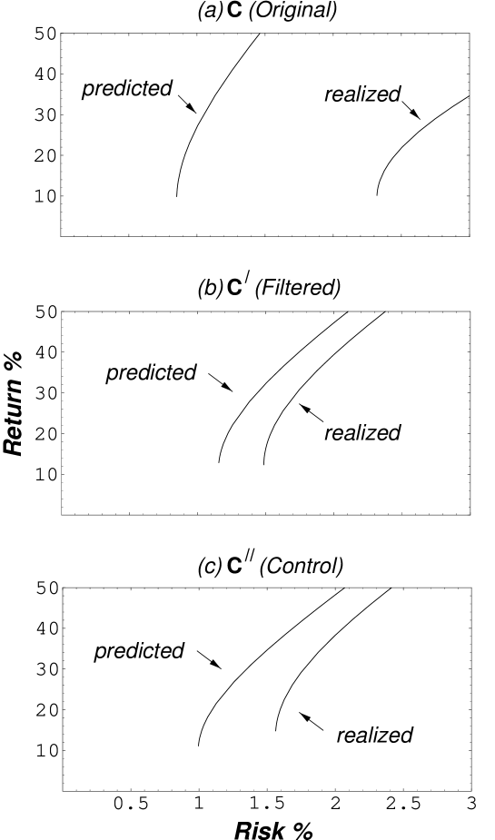
FIG. 1.: Portfolio return $R$ as a function of risk $D$ for the families of optimal portfolios constructed from (a) the original matrix C, (b) the filtered matrix C^′, and (c) the control C^′′. The curves on the left show the predicted level of risk, whereas the curves on the right show the realized risk $D$ calculated using the correlation matrix C^B for the second half of 1994. The ratio of realized to predicted risk is smallest for the RMT method (b), followed by the control (c), and largest for the original matrix (a)

FIG. 2.: Comparison of the realized risk for the family of portfolios constructed from C^′ (RMT method) and C^′′(conventional method). For a given return, the RMT portfolios are characterized by a lower level of risk than the the conventional portfolios.

FIG. 3.: Dependence of the realized risk on the number of eigenvalues kept in the calculation of the cleaned cross-correlation matrix C^′. For this plot, the level of realized return is chosen as 15% . RMT suggests that keeping 12 eigenvalues is the best choice for minimizing risk.

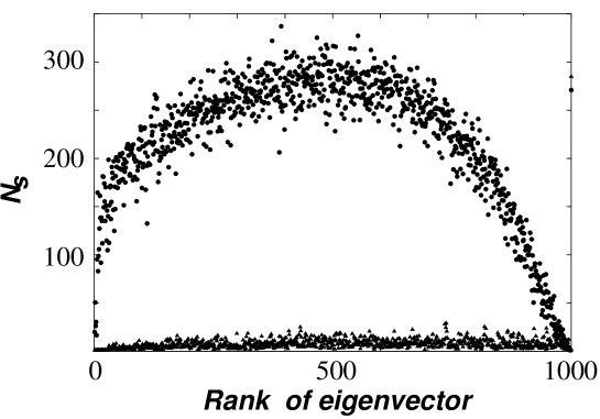
FIG. 4.: The number $N_{s}$ of significant components of the eigenvectors of C^A (circles) and C^′ (triangles) is plotted against the rank of the eigenvector. $N_{s}$ is defined as one over the inverse participation ratio. Most of the eigenvectors of C^A have a large $N_{s}$, whereas all but one of the eigenvectors of C^′ have a small $N_{s}$ indicating individually fluctuating stocks or interactions between small clusters of stocks. The last eigenvector with $N_{s}=285$ describes the influence of the whole market and corresponds to a long range ferromagnetic interaction in the magnetic analogy.

REFERENCES

- [1] S. Kirkpatrick, G. D. Gelatt and M. P. Vecchi, Science 220, 671 (1983).
- [2] G. Baskaran, Y. Fu, and P. W. Anderson, J. Stat. Phys. 45, 1 (1986).
- [3] M. Mézard and G. Parisi, Europhys. Lett. 2, 913 (1986).
- [4] G. F. Lima, A. S. Martinez, and O. Kinouchi, Phys. Rev Lett. 87, 010603 (2001)
- [5] S. Galluccio, J.-P. Bouchaud, and M. Potters, Physica A 259, 449 (1998).
- [6] E. J. Elton and M. J. Gruber, Modern Portfolio Theory and Investment Analysis (J. Wiley, New York, 1995).
- [7] L. Laloux et al, Phys. Rev. Lett. 83, 1469 (1999).
- [8] V. Plerou et al., Phys. Rev. Lett. 83, 1471 (1999).
- [9] P. Gopikrishnan et al., Phys. Rev. E 64, 035106(R) (2001); see also cond-mat/0011145.
- [10] F. Black and R. Litterman, Financial Analysts Journal September/October 1992, 28 (1992).
- [11] E. P. Wigner, Ann. Math. 53, 36 (1951).
- [12] T. Guhr, A. Müller-Groeling, and H. A. Weidenmüller, Phys. Reports 299, 189 (1998).
- [13] S. Drozdz et al, Physica A 287, 440 (2000).
- [14] J. D. Noh, Phys. Rev. E 61, 5981 (2000).
- [15] L. Laloux, Int. J. Theor. Appl. Finance 3, 391 (2000).
- [16] Z. Burda, et al. cond-mat/0103108.
- [17] P. Gopikrishnan et al., cond-mat/0108023.
- [18] Analyzed are data taken from the Trades and Quotes database published by the New York Stock Exchange, for the 1-year period 1994, recorded at 30-minute intervals. Only those companies that survive the entire period are considered in our analysis.
- [19] For a normalized eigenvector with components the IPR is defined as . The interpretation of the IPR can be made plausible by considering two limiting cases. For (i) a vector with equal components the IPR is , whereas for (ii) a vector with one component equal to one and all other components equal to zero the IPR is one. In both cases, the inverse of the IPR is the number of significant components.