The Hartree-Fock Based Diagonalization
- an Efficient Algorithm for the Treatment
of Interacting Electrons in Disordered Solids

Abstract

The Hartree-Fock based diagonalization is a computational method for the investigation of the low-energy properties of correlated electrons in disordered solids. The method is related to the quantum-chemical configuration interaction approach. It consists in diagonalizing the Hamiltonian in a reduced Hilbert space built of the low-energy states of the corresponding disordered Hartree-Fock Hamiltonian. The properties of the method are discussed for the example of the quantum Coulomb glass, a lattice model of electrons in a random potential interacting via long-range Coulomb interaction. Particular attention is paid to the accuracy of the results as a function of the dimension of the reduced Hilbert space. It is argued that disorder actually helps the approximation.

and

1 Introduction

In recent years there has been a strong interest in the electronic properties of correlated electrons in the presence of disorder, e.g., in connection with the fractional quantum Hall effect, heavy-fermion systems or the apparent metal-insulator transition of the two-dimensional electron gas in Si-MOSFETs. If both disorder and interactions are strong, the usual analytic theories often do not work well. For instance, a complete analytic description of the localized, insulating phase of disordered interacting electrons has not been achieved. Therefore, computational methods are particularly important in this area.

However, the numerical simulation of disordered many-particle systems is one of the most complicated problems in computational condensed matter physics. First, the size of the many-particle Hilbert space to be considered grows exponentially with the system size. Second, in the presence of disorder many samples with different disorder configurations have to be simulated in order to obtain averages or typical values of physical quantities. Since many interesting quantities like the conductance are non-self-averaging, often the entire distribution function of an observable is desired, requiring at least of the order of 10³ samples. Moreover, the basic interaction between the electrons, the Coulomb interaction, is long-ranged. While in the metallic phase it is often possible to use an effective model with screening already built in, the long-range Coulomb interaction has to be retained for a correct description of the insulating phase when screening breaks down. This drastically increases the numerical effort required.

One way to overcome the problem of the exponentially (in the number of particles) large Hilbert space is to use mean-field ideas to reduce the system to a self-consistent effective single-particle problem. The simplest way to do this are the Hartree and Hartree-Fock approximations (see [1, 2] for applications of the Hartree-Fock approximation to lattice models of disordered interacting electrons). In the more sophisticated form of the density functional theory this effective single-particle approach has proven to be successful in predicting the electronic structure of a wide variety of materials. In general, the effective single-particle methods permit the simulation of rather large systems ($>10^{3}$ sites) but the approximations involved are uncontrolled and can usually not be improved systematically. Effective single-particle methods usually work well on energy scales of eV. At low temperatures and energies of the order of meV electronic correlations become more important and new physical phenomena beyond the scope of effective single-particle theories emerge. Here methods are desired which give numerically exact results or which can be taken, at least in principle, to arbitrary accuracy. However, most of these methods are severely restricted when simulating disordered interacting electrons.

Exact diagonalization requires the diagonalization of a matrix whose dimension is that of the full many-particle Hilbert space. Therefore, it works only for very small systems (e.g., with up to about $4\times 4$ lattice sites in two dimensions) [3, 4]. For one-dimensional systems the density-matrix renormalization group (DMRG) method [5] is a very efficient tool to obtain the low-energy properties. It is, however, less effective in higher dimensions. Moreover, the long-range Coulomb interaction strongly complicates the original real-space based DMRG. Later, momentum-space based versions of the DMRG method have also been tested [6]. However, it turned out that their accuracy is generically less than that of the the real-space DMRG under favorable conditions [7]. Quantum Monte-Carlo [8] methods are another means of simulating disordered many-particle systems. They are very effective for bosons at finite temperatures. Very low temperatures are, however, hard to reach. Moreover, simulations of fermions suffer from the notorious sign problem, although this turned out to be less severe in the presence of disorder. Recently, the sign-problem could be further reduced using a multilevel blocking Monte-Carlo method [9].

In this paper we present an alternative method for simulating disordered interacting electrons, the Hartree-Fock based diagonalization (HFD). It is related to the configuration interaction method [10]. This is one of the early methods for treating interacting electrons which is particularly popular in quantum chemistry. We will show that the Hartree-Fock based diagonalization is a very suitable method for strongly disordered interacting electrons. In fact, the algorithm benefits from the presence of disorder. The remainder of this paper is organized as follows. In Sec. 2 we present the method and discuss its properties. In Sec. 3 we show the results of various test calculations for the quantum Coulomb glass Hamiltonian. Section 4 summarizes a few important physical results obtained using the HFD method. We conclude in Sec. 5.

2 Hartree-Fock based diagonalization

The Hartree-Fock based diagonalization (HFD) is similar to the configuration interaction method [10] used in quantum chemistry, but adapted for disordered lattice Hamiltonians. The main idea of the HFD is to diagonalize the Hamiltonian in a small subspace of the Hilbert space spanned by the low-energy eigenstates of the corresponding Hartree-Fock approximation. A schematic of the Hartree-Fock based diagonalization method is shown in Fig. 1.

do for each disorder configuration solve HF approximation construct many-particle HF states find lowest-in-energy HF states transform Hamiltonian to basis of low-energy HF states diagonalize Hamiltonian transform observables to HF basis and calculate their values enddo

Figure 1: Structure of the Hartree-Fock (HF) based diagonalization method.

The first step of the HFD method consists in solving the Hartree-Fock approximation of the Hamiltonian. Due to the presence of disorder this is a non-trivial single-particle problem which can only be solved numerically. In the second step many-particle Slater states are constructed from the single-particle states of the Hartree-Fock approximation. An elaborate Monte-Carlo algorithm is then used to find the many-particle states with the lowest energy expectation values. In the third step the Hamiltonian is transformed into the basis formed by these states and diagonalized. Finally, the operators of the desired observables are also transformed into the new basis, and their values are calculated.

Since the Hartree-Fock states are comparatively close in character to the exact eigenstates in the entire parameter space the Hartree-Fock based diagonalization works well for all parameters while related methods based on non-interacting or classical eigenstates [12, 13] instead of Hartree-Fock states are restricted to small parameter regions. The presence of strong disorder actually helps the method because it breaks possible symmetries in the Hamiltonian and lifts the related degeneracies of the eigenenergies which usually pose severe problems for Hartree-Fock calculations.

In the following we will illustrate the application of the HFD method for the example of the quantum Coulomb glass, a model of interacting electrons in a random potential. The model is defined on a regular hypercubic lattice with $\mathcal{N}=L^{d}$ ($d$ is the spatial dimensionality) sites occupied by $N=K\mathcal{N}$ electrons ($0\!<\!K\!<\!1$). To ensure charge neutrality each lattice site carries a compensating positive charge of $Ke$. The Hamiltonian is given by

$$H=-t\sum_{\langle ij\rangle}(c_{i}^{\dagger}c_{j}+c_{j}^{\dagger}c_{i})+\sum_{i}\varphi_{i}n_{i}+\frac{1}{2}\sum_{i\not=j}(n_{i}-K)(n_{j}-K)U_{ij}$$ (1)

where $c_{i}^{\dagger}$ and $c_{i}$ are the electron creation and annihilation operators at site $i$, respectively, and $\langle ij\rangle$ denotes all pairs of nearest neighbor sites. $t$ is the strength of the hopping term, i.e., it corresponds to the kinetic energy, and $n_{i}$ is the occupation number of site $i$. We parametrize the Coulomb interaction $U_{ij}=e^{2}/r_{ij}$ by its value $U$ between nearest neighbor sites. For a correct description of the insulating phase the Coulomb interaction has to be kept long-ranged, since screening breaks down in the insulator. The random potential values $\varphi_{i}$ are chosen independently from a box distribution of width $2W_{0}$ and zero mean. For $U_{ij}=0$ the quantum Coulomb glass becomes identical to the Anderson model of localization and for $t=0$ it turns into the classical Coulomb glass. We note that (1) describes a system of spinless electrons. However, the inclusion of the electron spin is straightforward (see Sec. 4; it just doubles the number of degrees of freedom).

We now give a more detailed description of the HFD method for the quantum Coulomb glass. For each disorder configuration the first step consists in numerically diagonalizing the Hartree-Fock approximation

$$H_{\rm HF}= -t \sum_{\langle ij\rangle}(c_{i}^{\dagger}c_{j}+c_{j}^{\dagger}c_{i})+\sum_{i}\varphi_{i}n_{i}$$ (2)

$$+ \sum_{i\not=j}n_{i}~{}U_{ij}\langle n_{j}-K\rangle-\sum_{i,j}c_{i}^{\dagger}c_{j}~{}U_{ij}\langle c_{j}^{\dagger}c_{i}\rangle,$$

of the Hamiltonian as described in Ref. [2]. Here $\langle\ldots\rangle$ represents the expectation value with respect to the Hartree-Fock ground state which has to be determined self-consistently. This calculation results in an orthonormal set of single-particle Hartree-Fock states $|\psi_{\nu}\rangle=b_{\nu}^{\dagger}|0\rangle$ which defines a unitary transformation $b_{\nu}^{\dagger}=\sum_{i}S_{\nu i}c_{i}^{\dagger}$ .

In the second step of the HFD method we construct many-particle states, i.e., Slater determinants,

$$|\{\nu\}\rangle=b_{\nu_{1}}^{\dagger}\ldots b_{\nu_{N}}^{\dagger}|0\rangle~{}.$$ (3)

Note that for the two limiting cases mentioned above, i.e for the Anderson model of localization and for the classical Coulomb glass, these states are also eigenstates of the full Hamiltonian (1). We then determine the set of many-particle states (3) which have the lowest expectation values $\langle\{\nu\}|H|\{\nu\}\rangle$ of the energy. This set varies from disorder realization to disorder realization in a non-trivial way making it difficult to use an efficient deterministic algorithm for this task. Since the total number of states is too high for a complete enumeration we employ a Monte-Carlo method. It is based on the thermal cycling method [11] in which the system is repeatedly heated and cooled. In addition, at the end of each cycle a systematic local search around the current configuration is performed. While performing the Monte-Carlo simulation we keep an archive containing the $B$ states with the lowest energies encountered so far. When no new low-energy states have been found for a certain number of Monte-Carlo steps we stop. The set of low-energy many-particle states found in this way spans the sub-space of the Hilbert space relevant for the low-energy properties. Its dimension $B$ determines the accuracy of the results. (If we choose $B$ equal to the full Hilbert space dimension the results will be exact since all we have done is a unitary transformation).

The third HFD step consists in transforming the Hamiltonian from the original site representation to the Hartree-Fock representation and calculating the matrix elements $\langle\{\nu\}|H|\{\mu\}\rangle$. The resulting Hamiltonian matrix $H_{\{\nu\}\{\mu\}}$ of size $B\times B$ is then diagonalized using standard library routines. Note that $H_{\{\nu\}\{\mu\}}$ is usually not very sparse: if $|\{\nu\}\rangle$ and $|\{\mu\}\rangle$ differ in the occupation of at most 4 single-particle states, the matrix element is non-zero. Moreover, number and position of the non-zero matrix elements differ between different disorder configurations. Thus, specialized codes for sparse matrices will not increase the performance significantly. The diagonalization gives the eigenenergies and the eigenstates in the Hartree-Fock basis $|\{\nu\}\rangle$. In order to calculate physical observables like occupation numbers or transport properties we transform their operators to the Hartree-Fock representation. This is usually faster than transforming the eigenstates states back to site or momentum representation.

3 Test calculations for the quantum Coulomb glass model

In order to test the method and to check the dependence of the results on the size $B$ of the basis we have carried out extensive simulations for systems with $4\times 4$ sites. We have compared the results to those of exact diagonalizations which are easily possible for spinless electrons on a $4\times 4$ lattice. First we have investigated the dependence of the ground state energy $E_{0}^{B}$ on $B$ and compared it with the exact result $E_{0}$. A typical example of such a calculation for one particular disorder realization is presented in Fig. 2.

Figure 2: Dependence of the ground state energy $E_{0}^{B}$ and its relative error $(E_{0}^{B}-E_{0})/E_{0}$ on the size $B$ of the basis used for a system of 8 electrons on $4\times 4$ sites, $W_{0}=1,~{}t=0.1,~{}U=1$. The solid line in the inset is a fit to an exponential law. For comparison, the energy of the first excited state is $E_{1}=-24.73$.

As usual the ground state energy is not very sensitive to the accuracy of the approximation. Already the relative energy error of the Hartree-Fock approximation ($B=1$ in Fig. 2) is as low as $2*10^{-4}$. This is about 2.5% of the energy separation between the ground and the first excited state. Keeping a basis size of 300 within the HFD method reduces the error by a factor of 10. Further increasing the basis size to 1000 (which is still less than 10% of the total Hilbert space dimension of 12870) gives a relative error of less than $10^{-6}$. For the basis sizes covered in our calculation the convergence of the ground state energy is approximately exponential (see inset of Fig. 2).

Since the ground state energy is not a very sensible indicator to judge the quality of the approximate ground state we also studied the overlap between the approximate and the exact eigenstates. Results for one disorder realization for several parameter sets are shown in Fig. 3.

Figure 3: Overlap between the HFD eigenstates and the corresponding exact eigenstates for a system of 8 electrons on $4\times 4$ sites, $W_{0}=1,~{}U=1$ and several values of $t$. Ground state: $\circ$, 1st to 4th excited state: $\square\bigtriangleup\oplus\times$. Note that the overlap axis has a quadratic scale.

In all cases a basis size of $B=100$ is sufficient to achieve an overlap larger than 0.99 between the approximate and the exact ground states. The approximation works very well for small $t$ because the system is close to the classical limit ($t=0$) where the Hartree-Fock approximation will become exact. It will also work well for $t\gg 1$ when the system approaches the non-interacting limit because the Hartree-Fock approximation is exact in this limit, too. The excited states in general converge slower than the ground state. For $t=0.3$ and 0.5 a basis size of $B=100$ is not sufficient to obtain more than the first excited state with an accuracy comparable to that of the ground state.

In addition to the ground state energy and the overlaps between the approximate and exact eigenstates we have investigated the convergence properties of several ground state expectation values. Figure 4 shows the convergence of the occupation numbers as a function of basis size $B$ for the same system as in Fig. 2.

Figure 4: Ground state occupation numbers $\langle n_{i}\rangle$ of selected sites $i$ vs. basis size $B$ for a system of 8 electrons on $4\times 4$ sites, $W_{0}=1,~{}t=0.1,~{}U=1$.

While some of the occupation numbers have significant errors within Hartree-Fock approximation, the HFD method with a basis size of 100 gives all occupation numbers with a satisfactory accuracy of better than $10^{-2}$.

As a last example for the comparison between HFD and exact results we want to discuss the frequency dependent conductance. It is calculated from the Kubo-Greenwood formula [15] which relates the conductance to the current-current correlation function in the ground state. Using the spectral representation of the correlation function the real (dissipative) part of the conductance (in units of the quantum conductance $e^{2}/h$) is obtained as

$$\Re~{}G^{xx}(\omega)=\frac{2\pi^{2}}{\omega}L^{d-2}\sum_{\alpha}|\langle 0|j^{x}|\alpha\rangle|^{2}\delta(\omega+E_{0}-E_{\alpha})$$ (4)

where $j^{x}$ is the $x$ component of the current operator and $\alpha$ denotes the eigenstates of the Hamiltonian. The finite life time $\tau$ of the eigenstates in a real d.c. transport experiment results in an inhomogeneous broadening $\gamma=1/\tau$ of the $\delta$ functions in the Kubo-Greenwood formula. Here we have chosen $\gamma=0.05$ which is of the order of the single-particle level spacing. While we expect the conductance values to slightly vary with $\gamma$ the qualitative dependence on disorder or interaction strength will be independent of the broadening value. According to eq. (4) the accuracy of the conductance depends not only on the accuracy of the ground state but also on that of the excited states. For this reason, the conductance is very sensitive to the quality of the approximation. Figure 5 shows the relative error of the conductance as a function of the basis size $B$ for different frequencies and parameter sets (for one particular disorder realization).

Figure 5: Relative error of the conductance $G(\omega)$ as a function of basis size $B$ for a system of 8 electrons on $4\times 4$ sites, $W_{0}=1,~{}U=1$. Upper row: $t=0.1$, different frequencies ($\lambda$ is the number of the contributing excited state), lower row: contribution of the first excited state for different $t$.

Clearly, the convergence of the conductance is much slower than that of the other quantities considered so far. However, a basis size of $B=300$ is sufficient to reduce the error to a few percent in all cases. The upper row in Fig. 5 also shows that the convergence becomes slower at higher frequencies. This is to be expected since higher excited states are necessary to calculate the conductance at higher frequency. We have carried out similar test calculations for other observables of interest like the single-particle density of states and the return probability of single-particle excitations [16]. Since these quantities also involve excited states their convergence properties are overall very similar to that of the conductance.

We now turn to the question how to judge the quality of the approximation for larger systems sizes when no exact diagonalization results are available for comparison. In this case we use a heuristic method. We carry out several calculations with increasing basis sizes and check how much the results change. If this change becomes sufficiently small we stop. In Fig. 6 such a series of calculations is shown for the conductance of a system of 18 electrons on $6\times 6$ lattice sites. The dimension of the full Hilbert space is $9.1*10^{9}$.

Figure 6: Conductance as a function of frequency for a system of 18 electrons on $6\times 6$ sites, $W_{0}=1,~{}t=0.1,~{}U=0.1$. The data points represent logarithmic averages over 400 disorder realizations.

The figure shows that with too small a basis ($B=10$) the low-frequency conductance values are too small by a sizeable factor of around 3. However, already a basis size of $B=100$ gives a very small error for frequencies smaller than $\omega=0.2$. A further increase of $B$ leaves the low-frequency part of the conductance curve essentially unchanged but systematically improves the results at higher frequencies. This happens because higher excited states are responsible for the conductance at higher frequency. With increasing basis size more and more of these states can be calculated with sufficient accuracy.

4 Selected results obtained with the HFD method

In the last few years we have used the HFD method to study various transport and localization properties of interacting electrons in a random potential. The interest in this topic resurged during the 1990’s because new experimental and theoretical results had cast doubt on the established theories based on perturbation theory for weak disorder and interactions. In this section we will briefly summarize a few of the key results obtained.

Since a realistic description has to include the spin degrees of freedom we have generalized the quantum Coulomb glass (1) to electrons with spin. A system with $\mathcal{N}$ lattice sites now contains $N=N_{\uparrow}+N_{\downarrow}=2K\mathcal{N}$ electrons ($0\!<\!K\!<\!1$) and has a compensating positive charge of $2Ke$ on each lattice site. The Hamiltonian is given by

$$H = -t\sum_{\langle ij\rangle,\sigma}(c_{i\sigma}^{\dagger}c_{j\sigma}+c_{j\sigma}^{\dagger}c_{i\sigma})+\sum_{i,\sigma}\varphi_{i}n_{i\sigma}$$

$$+~{}\frac{1}{2}\sum_{i\not=j,\sigma,\sigma^{\prime}}U_{ij}~{}(n_{i\sigma}-K)(n_{j\sigma^{\prime}}-K)+U_{\rm H}\sum_{i}n_{i\uparrow}n_{i\downarrow}$$

where $c_{i\sigma}^{\dagger}$, $c_{i\sigma}$, and $n_{i\sigma}$ are the creation, annihilation and occupation number operators for electrons at site $i$ with spin $\sigma$. Two electrons on the same site interact via a Hubbard interaction $U_{\rm H}$.

Figure 7 shows the typical conductance values of a system of $4\times 4$ lattice sites at half filling as a function of the interaction $U$ for different hopping matrix elements $t$.

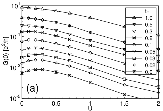
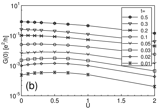
Figure 7: d.c. conductance $G(0)$ as a function of interaction $U$ for a system of $4\times 4$ sites occupied by (a) 8 spin-up and 8 spin-down electrons and (b) 8 spinless fermions. The Hubbard energy is $U_{H}=U$, and the HFD basis size is $B=500$. The inhomogeneous broadening is $\gamma=0.0625$.

Panel (a) shows results for an occupation of 8 spin-up and 8 spin-down electrons while panel (b) is for 8 spinless fermions. Since the logarithm of the conductance rather than the conductance itself is a self-averaging quantity in a disordered system, we calculate the typical conductance by averaging the logarithms of the conductances of 1000 (400 in the spinless case) disorder configurations. The data show that weak electron-electron interactions reduce the d.c. conductance for large kinetic energy $t$. For small $t$, i.e., in the localized regime, small and moderate interactions significantly enhance the d.c. conductance. For larger interaction strength the conductance drops no matter what $t$ is, indicating the crossover to a Wigner crystal or Wigner glass. The data also show that the spin degrees of freedom do not change the qualitative behavior in the parameter region investigated. In fact, after rescaling the conductance of the system with spins by 1/2 and the interaction strength by 2 the two sets of curves nicely fall on top of each other within the statistical accuracy. Therefore we conclude that for the systems considered the Coulomb interaction plays the essential role for the delocalizing tendency for weak interactions as well as for the localizing tendency for strong interactions.

In addition to the conductance we have also studied the localization properties of single-particle excitations which we characterize by the single-particle return probability [17]

$$R_{\sigma}(\omega)=\frac{1}{g(\omega)}\frac{1}{\mathcal{N}}\sum_{i}\lim_{\delta\to 0}\frac{\delta}{\pi}\,G_{i\sigma i\sigma}^{R}(\omega+i\delta)\,G_{i\sigma i\sigma}^{A}(\omega-i\delta).$$ (6)

Here $G_{i\sigma j\sigma^{\prime}}^{R,A}(\omega)$ are the retarded and advanced single-particle Greens functions. $g(\omega)$ denotes the single-particle density of states. In an interacting system the return probability (6) entangles localization and decay information, since $R_{\sigma}$ is decreased from 1 not only by delocalization but also by decay of the quasi-particles. In order to extract the localization of the quasi-particles we normalize $R_{\sigma}(\omega)$ by the square of the quasiparticle weight, $Z_{\sigma}(\omega)$. The resulting normalized return probability is presented in Fig. 8.

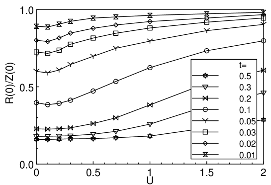
Figure 8: Normalized single-particle return probability at the Fermi energy, $R_{\sigma}(0)/Z_{\sigma}(0)$ for a system of $4\times 4$ sites occupied by 8 spin-up and 8 spin-down electrons. The parameters are as in Fig. 7

The figure shows that, in general, interactions tend to localize the single-particle excitations. The delocalization at low interaction strength and small kinetic energy is a much smaller effect than the corresponding increase in the conductance discussed above. This is in agreement with earlier results [2] based on the Hartree-Fock approximation. The reason for the strong single-particle localization is the Coulomb gap in the single-particle density of states which effectively reduces the overlap between excitations close to the Fermi level. The density of states of the particle-hole excitations responsible for the conductance has a much weaker gap, if any.

For a more detailed presentation of our results see, e.g., Refs. [18, 19, 20] for studies of spinless fermions in one, two and three dimensions or Ref. [21] for investigations of electrons with spin.

5 Summary and conclusions

In this paper we have discussed an efficient numerical method, the Hartree-Fock based diagonalization, for the simulation of interacting electrons. It is based on diagonalizing the Hamiltonian in a subspace of the Hilbert space spanned by the low-energy Hartree-Fock eigenstates. The method is very general, we have used it to study a variety of systems including quantum nano-structures [22]. However, it is particularly suited for the investigation of strongly disordered systems because the disorder lifts most of the degeneracies which complicate the application of the Hartree-Fock approximation and thus also the Hartree-Fock based diagonalization.

We have presented an evaluation of the method for the example of the quantum Coulomb glass, a lattice model of interacting electrons in a random potential. We have shown that the ground state occupation numbers and the ground state energy converge very rapidly with increasing size of the subspace used. The convergence of the ground state energy is approximately exponential in the parameter range studied. The convergence of dynamic observables whose calculation involves excited states is less quick. However, we were able to achieve satisfactory accuracy with very small subspace sizes.

In the last few years we have used the Hartree-Fock based diagonalization to investigate a variety of transport and localization properties of strongly disordered interacting electrons. We have calculated the conductance, the charge stiffness and various localization properties of single-particle excitations. We found that weak electron-electron interactions tend to increase the transport in the localized regime but decrease the transport in the metallic regime. Sufficiently strong interactions always localize the system which then forms a Wigner crystal or a Wigner glass.

This work was supported in part by the German Research Foundation under grant no. SFB 393/C2.

References

- [1] M. Milovanovic, S. Sachdev, and R.N. Bhatt, Phys. Rev. Lett. 63, 82 (1989); G. Bouzerar and D. Poilblanc, J. Phys. (Paris) I 7, 877 (1997)
- [2] F. Epperlein, M. Schreiber, and T. Vojta, Phys. Rev. B 56, 5890 (1997); phys. stat. sol. (b) 205, 233 (1998)
- [3] E. Dagotto, Rev. Mod. Phys. 66, 763 (1994); R. Berkovits and Y. Avishai, Phys. Rev. Lett. 76, 291 (1996)
- [4] T. Vojta, F. Epperlein, and M. Schreiber, phys. stat. sol. (b) 205, 53 (1998)
- [5] S. R. White, Phys. Rep. 301, 187 (1998)
- [6] T. Xiang, Phys. Rev. B 53, 10445 (1996)
- [7] S. Nishimoto et al., cond-mat/0110420
- [8] W. von der Linden, Phys. Rep. 220, 53 (1992)
- [9] R. Egger, W. Haeusler, C.H. Mak, and H. Grabert, Phys. Rev. Lett. 82, 3320 (1999)
- [10] P. Fulde, Electron correlations in molecules and solids, Springer, Berlin (1995)
- [11] A. Möbius, A. Neklioudov, A. Diaz-Sanchez, K.H. Hoffmann, A. Fachat, and M. Schreiber, Phys. Rev. Lett. 79, 4297 (1997)
- [12] A. L. Efros and F. G. Pikus, Solid State Commun. 96, 183 (1995)
- [13] J. Talamantes, M. Pollak, and L. Elam, Europhys. Lett. 35, 511 (1996)
- [14] S. V. Kravchenko et al., Phys. Rev. Lett. 77, 4938 (1996)
- [15] K. Kubo, J. Phys. Soc. Jpn. 12, 576 (1957); D. A. Greenwood, Proc. Phys. Soc., London 71, 585 (1958)
- [16] F. Epperlein, Numerische Simulation des Transport in ungeordneten Vielelektronensystemen, Dissertation, Technische Universität Chemnitz (1999)
- [17] E.N. Economou and M.H. Cohen, Phys. Rev. Lett. 25, 1445 (1970)
- [18] T. Vojta, F. Epperlein, and M. Schreiber, Phys. Rev. Lett 81, 4212 (1998)
- [19] M. Schreiber, F. Epperlein, and T. Vojta, Physica A 266, 443 (1999)
- [20] T. Vojta and F. Epperlein, Ann. Phys. (Leipzig) 7, 493 (1998)
- [21] T. Vojta and M. Schreiber, Phil. Mag. B 81, 1117 (2001)
- [22] J. Siewert, M. Schreiber, and T. Vojta, in Proc. 25th Int. Conf. Physics of Semiconductors, N. Miura and T. Ando (Eds.), Springer Proceedings in Physics 87, 1061 (2001)