Spectral Properties of High-T_c Cuprates via a Cluster-Perturbation Approach

Abstract

Angular-resolved photoemission data on half-filled doped cuprate materials are compared with an exact-diagonalization analysis of the three-band Hubbard model, which is extended to the infinite lattice by means of a perturbation in the intercluster hopping (cluster perturbation theory). A study of the band dispersion and spectral weight of the insulating cuprate Sr₂CuO₂Cl₂ allows us to fix a consistent parameter set, which turns out to be appropriate at finite dopings as well. In the overdoped regime, our results for the spectral weight and for the Fermi surface give a good description of the experimental data on Bi₂Sr₂CaCu₂O_8+δ. In particular, the Fermi surface is hole-like and centered around $k=(\pi,\pi)$. Finally, we introduce a hopping between two layers and address the issue of bilayer splitting.

PACS numbers: 74.72.-h, 74.72.Hs, 79.60.-i.

1 INTRODUCTION

Angle-resolved photoemission spectroscopy (ARPES) has provided significant insight into the single-particle properties of high-temperature superconductors (HTSC), providing a measure of the $k$-dependent spectral function below the Fermi surface, which is suitable for a direct comparison with theoretical models. Recently, particular attention has been devoted to the spectral properties of undoped antiferromagnetic parent compounds of the HTSC, mainly Sr₂CuO₂Cl₂ due to its ideal experimental characteristics. A series of photoemission measurements [1, 2, 3] of these half-filled cuprates provides a detailed view of the quasiparticle dispersion of the highest electron-removal state, commonly known as the Zhang-Rice-Singlet (ZRS) [4]. In a number of previous works, the wave-vector dependence of this band has been theoretically analyzed on basis of exact-diagonalization (ED) and quantum monte-carlo (QMC) studies of Hubbard [5], t-J [6] and three-band models [7, 8, 9]. On the other hand, it is clear that an appropriate inclusion of the most relevant orbitals (Cu3d${}_{x^{2}-y2}$, O2p_x and O2p_y) of the CuO₂ unit cell, i. e., based on the three-band Hubbard model should provide a more complete description of the system. The trouble is that an exact-diagonalization analysis of this model has to be necessarily restricted to a rather limited number of unit cells, due to the rapid increase of the size of the Hilbert space. Even QMC simulations of larger systems were still severly restricted, providing informations on only a few k-points in the Brillouin zone.

To remedy this problem, we follow here the idea [10] of extending the results of the exact diagonalization of a small cluster to the whole lattice within a lowest-order perturbation in the intercluster hopping. This technique has been shown to produce quite good results for the Hubbard [10] model and has been successfully applied to the study of the stripe phase in the cuprate materials [11, 12]. It has the advantage to treat accurately short-range correlations, which are believed to be the most important ones in these systems [13]. Furthermore, at the same time, it accesses all $k$ points of the Brillouin zone, while in ordinary ED only few $k$ points are available. This last property is, of course, crucial if one wants to analyze a dispersion or determine a Fermi surface with sufficient details.

As a matter of fact, recent advances in experimental ARPES techniques allowed for a direct mapping of the Fermi surface, which has been experimentally analyzed in detail in overdoped Bi₂Sr₂CaCu₂O_8+δ (Bi2212) [14, 15, 16, 17, 18, 19, 20]. Unfortunately, there seems to be disagreement between results obtained at different photon energies. Measurements taken at a photon energy of 22eV typically show a Fermi surface closed around ${\bf k}=(\pi,\pi)$ (”hole-like”), whereas at 33eV photon energy the same materials show a shape closed around ${\bf k}=(0,0)$ (”electron-like”). To understand this issue, we extend our analysis to an overdoped system with 25 % doping, where we keep the same parameters obtained at half filling. Our results give a quasiparticle dispersion which is compatible with the experiments on the overdoped cuprates, exhibiting a hole-like Fermi surface closed around ${\bf k}=(\pi,\pi)$.

In the final part of the paper, we present results obtained by coupling two layers with an interlayer hopping $t_{\perp}=0.1t_{pd}$, and study its effects on the Fermi-surface splitting, comparing with experimental results.

2 MODEL AND TECHNIQUE

Common property of all HTSC and of their parent compounds is the presence of stacked CuO₂ layers. The general agreement is that the relevant excitations of these materials take place within these layers. A generic model considers three relevant orbitals, namely, Cu${}_{d_{x^{2}-y^{2}}}$, O${}_{p_{x}}$ and O${}_{p_{y}}$ orbitals[21, 13, 22]. Restricting to the on-site Coulomb interactions within the $d$ copper orbitals only, this gives the three-band Hubbard Hamiltonian [23]

$$H_{3b} = -t_{pd}\sum_{\left<ij\right>,\sigma}\alpha_{ij}\left(d^{\dagger}_{i,\sigma}p_{j,\sigma}+p^{\dagger}_{j,\sigma}d_{i,\sigma}\right)$$ (4)

$$-t_{pp}\sum_{\left<jj^{\prime}\right>,\sigma}\alpha^{\prime}_{jj^{\prime}}\left(p^{\dagger}_{j,\sigma}p_{j^{\prime},\sigma}+p^{\dagger}_{j^{\prime},\sigma}p_{j,\sigma}\right)$$

$$+\frac{U_{d}}{2}\sum_{i,\sigma,\sigma^{\prime}}d^{\dagger}_{i,\sigma}d_{i,\sigma}d^{\dagger}_{i,\sigma^{\prime}}d_{i,\sigma^{\prime}}$$

$$+\Delta\sum_{j,\sigma}p^{\dagger}_{j,\sigma}p_{j,\sigma},$$

where the operators $d^{\dagger}_{i\sigma}$ and $p^{\dagger}_{j,\sigma}$ create holes in the Cu 3d and in the O 2p orbitals, respectively, and $\alpha_{ij}$ and $\alpha^{\prime}_{jj^{\prime}}$ give the usual orbital phase factors. $\left<...\right>$ denotes summation over nearest neighbours.

Exact diagonalizations of $H_{3b}$ are usually limited to $4$ unit cells, allowing for just $3$ inequivalent wave vectors, which are not enough to address questions of quasiparticle dispersion or of Fermi surface. Nevertheless, since the important correlations of these strongly-correlated materials should be relatively short range (a celebrated example is the Zhang-Rice singlet [4]) one can still envisage to capture these short-range correlations by exact diagonalization of a small cluster, and then continue the cluster properties to the infinite lattice within a perturbation in the inter-cluster hopping elements. This idea has been suggested by Sénéchal and coworkers[10] and has been termed “Cluster-Perturbation Theory”(CPT). A closely related method has been previously suggested to treat the coupling between one-dimensional Luttinger liquids, and to address the problem of the crossover from one to higher dimensions [24, 25, 26].

Central piece of this method is the Green function of the cluster $G_{ij\sigma}(z)$, which is obtained from Lanczos diagonalization. At the lowest order in the CPT, the full cluster Green’s function is non-diagonal in the momenta, as the partition into clusters produces a smaller “superlattice” Brillouin zone (BZ). More specifically, one has

$${\cal G}^{CPT}_{{{\bf q}+{\bf G}_{1}},{{\bf q}+{\bf G}_{2}},\sigma}(z)=\frac{1}{N_{0}}\sum_{{\bf r}_{1},{\bf r}_{2}}^{cluster}e^{i{\bf q}\cdot\left({{\bf r}_{1}}-{{\bf r}_{2}}\right)}e^{i{\bf G}_{1}\cdot{{\bf r}_{1}}-i{\bf G}_{2}\cdot{\bf r}_{2}}{\cal G}_{{\bf r}_{1},{\bf r}_{2},\sigma}({{\bf q}},z)\;,$$ (5)

where ${\bf G}_{i}$ are vectors of the reciprocal superlattice, ${\bf r}_{i}$ are cluster sites, ${\bf q}$ is restricted within the superlattice BZ, and $N_{0}$ is the number of unit cells of the cluster. Here, the cluster Green’s Function in the superlattice representation ${\cal G}_{{\bf r}_{1},{\bf r}_{2},\sigma}({{\bf q}},z)$ can be written as

$${\cal G}_{{\bf r}_{1},{\bf r}_{2},\sigma}({{\bf q}},z)=\left[{{\bf G}}_{\sigma}(z)^{-1}-{{\bf V}}({{\bf q}})\right]^{-1}_{{\bf r}_{1},{\bf r}_{2}}\;,$$ (6)

where both the cluster Green’s function ${{\bf G}}_{\sigma}(z)$ as well as the Fourier-transformed intercluster hopping $\bf{V({\bf q})}$ are $N_{0}\times N_{0}$ matrices in the cluster-site indices. $V({\bf q})$ is the only term connecting different clusters and, thus, displaying a ${\bf q}$-dependence. More specifically, let $T_{{\bf r}_{1},{\bf r}_{2}}({\bf\Delta})$ be the amplitude of hopping of a particle from a site ${\bf r}_{1}$ in cluster ${\bf R}$ and a site ${\bf r}_{2}$ in cluster ${\bf R}+{\bf\Delta}$ (which, for a translation-invariant system, only depends on the relative position, ${\bf\Delta}$, of the two clusters) then ${\bf V}({\bf q})$ is given by

$$V({\bf q})_{{\bf r}_{1},{\bf r}_{2}}=\sum_{{\bf\Delta}}e^{-i{\bf q}\cdot{\bf\Delta}}\ T_{{\bf r}_{1},{\bf r}_{2}}({\bf\Delta})\;.$$

This method obviously allows for a perturbative treatment of intracluster hopping terms as well. These can be included via the intercluster part $T_{{\bf r}_{1},{\bf r}_{2}}({\bf\Delta}={\bf 0})$. This gives the possibility of diagonalizing the cluster with periodic boundary conditions (BC), which is, clearly, more convenient numerically, but which contains unphysical hopping terms within the cluster. These additional terms, which are not present in the original problem, are then removed perturbatively via a $T_{{\bf r}_{1},{\bf r}_{2}}({\bf\Delta}={\bf 0})$ term with the opposite sign.

The non-diagonal terms ${\bf G}_{1}\not={\bf G}_{2}$ in Eq. (5) are produced by the different treatment of the intra- and intercluster hopping terms. Within the CPT, these terms are neglected, and one takes only the ${\bf G}_{1}={\bf G}_{2}$ part of the Green’s function to evaluate the spectral properties. Of course, in our multiband Hubbard model, the Green’s function is additionally a $3\times 3$ matrix in the orbitals of a single cell. The spectral function plotted in figures 1 and 2 is given by the sum of the diagonal elements of the Green’s-function matrix.

Notice, that the lowest-order CPT becomes exact in the trivial case of vanishing intercluster hopping and for non-interacting systems. This is due to the fact that corrections to Eq. (5) with Eq. (6) are given by higher-order cumulants, which are vanishing when Wick’s theorem holds, i. e. for non-interacting electrons. This fact makes the CPT an appealing interpolation between the strong- and the weak-coupling limits.

Our cluster consists of $N_{0}=2\times 2$ unit cells of the $3$-band model, for a total of $12$ lattice sites. For a single doped hole, the calculation of the Green’s Function requires 156 diagonalizations of $H_{3b}$ with at most 48400 basis states.

In principle, if we require that the hole density of the cluster fixes the doping of the system, the lowest doping we that can treat (beyond half filling) is $\delta=\frac{1}{4}$. Even so, we have to average the Green’s function between the two situations where the additional particle in the cluster has spin up or down.

As a matter of fact, one can also treat any doping between $\delta=0$ and $\delta=25\%$, by considering the cluster as being in a grand-canonical ensemble with fixed chemical potential $\mu$ between hole numbers $n_{h}=4$ and $n_{h}=4+1$. For finite temperature $T$, one can always fine-tune $\mu$ so that the average $n_{h}$ is the desired one $n_{h}=4(1+\delta)$. In the $T\to 0$ limit, this is obtained by using as a cluster Green’s function to insert in Eq. (6) the weighted sum of the two Green’s functions at $n_{h}=4$ and $n_{h}=5$ ($G_{n=4}$ and $G_{n=5}$, respectively), i. e., $G_{<n_{h}>=4+x}=x\ G_{n_{h}=5}+(1-x)\ G_{n_{h}=4}\quad\quad$ ( with $0\leq x\leq 1$), at the appropriate chemical potential. This is, physically, what one expects to occur in a cluster embedded in a larger system with $\delta=\frac{x}{4}$, namely, the particle number of the cluster $n$ will mainly fluctuate between $n=4$ and $n=5$.

3 RESULTS

First, we will discuss the dispersion of the highest electron removal states on the basis of the most recent experimental studies of the half-filled cuprate Sr₂CuO₂Cl₂. Up to few exceptions [3], these studies provide a consistent picture of the quasiparticle dispersion of the HTSC parent compounds [1, 2], showing two parabolas centered at $k=(\pi/2,0)$ and $k=(\pi/2,\pi/2)$. A characteristic energy difference $\Delta_{a}\approx 100-150meV$ between the maxima of the parabolas is observed. The total width W of the first band is about $300-400meV$ (compare figure 1 for experimental data). In accordance with earlier numerical studies [7, 8, 9, 21] of the three-band model, we find that the parameter set $t_{pp}=0.4t_{pd}$ , $U=6t_{pd}$ and $\Delta=4t_{pd}$ gives the best agreement with the experimental band structure. With the value of the copper-copper hopping matrix element[21] taken from the literature, $t_{pd}=1.3eV$, our calculations yield $\Delta_{a}=150meV$ and $W=400meV$. For the charge transfer gap we get $\Delta_{ct}=1.8eV$ in good agreement with the experimental value of $1.5-2eV$ [27, 28]. All these quantities are well within the margins of the experimental constraints. Therefore, these parameters should give a rather good description of the materials.

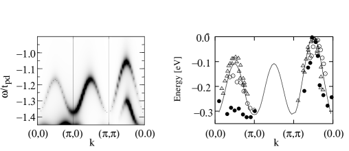
Figure 1: Grayscale plot of the spectral density of the half filled three-band Hubbard model, Eq. (4), with $t_{pp}=0.4$, $U_{d}=6$ and $\Delta=4$ (in units of $t_{pd}=1.3eV$), as obtained from CPT (left). The points mark the peak positions. The right panel shows the band dispersion obtained from different experiments (circles [1], filled circles [20] and triangles [2]).

Figure 1 shows a density plot of the single-particle spectral function $A(k,\omega)$ along the high-symmetry directions of the Brillouin zone (left panel). On the right panel we show corresponding ARPES data for comparison[3, 1, 2]. The dispersion of the band is reproduced quite well by our calculation. On the other hand, the spectral weight is too strong in the region $(\pi,0)$ to $(\pi,\pi)$, and too weak in the region between $(0,0)$ to $(\pi,0)$. This apparent disagreement is discussed in more detail below. Note that the scale of the binding energy is not absolute, since we are dealing with insulators.

We now comment on previous analyses of the experimental band dispersion displayed in Fig. 1 which have been based on the t-J model. This model is believed to be an effective low-energy version of the three-band Hubbard model[29]. The t-J model is more appropriate for numerical analysis, since his Hilbert space is smaller for a given number of unit cells. However, our results obtained by a CPT analysis of the three-band Hubbard model clearly differs from what one generally obtains from the t-J model. The latter predicts, in contrast to experiments, a flat band close to the Fermi energy at $(\pi,0)$ and $(\pi,0)-(0,\pi)$ [30]. A solution to this shortcoming of the t-J model has been suggested, by introducing longer-range hopping and interaction terms. In fact, a mapping of the three-band Hubbard model into a generalized t-J model has been recently proposed [31], which is consistent with results of the self-consistent Born approximation calculations and experimental data [32, 30, 33]. In particular, these latter results exhibit a dispersion in excellent agreement with our calculations of Fig. 1.

From Fig. 1, one can see that our calculation underestimates the spectral weight along $(0,0)-(\pi,0)$, which is usually strong in ARPES. One reason could be related to the small cluster in which the self-energy is evaluated, which takes only partially into account the electron correlations. Moreover, it was established numerically [10] that quasiparticles contained in the cluster are reproduced correctly, but they loose coherence over the cell boundary. Alternatively, the different spectral weight could be caused by intrinsic limitation of the model. For example, neglected orbitals [34] – although distant in energy – could possible give significant contributions to the spectral weight.

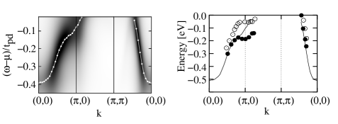
Figure 2: Spectral density of the overdoped ($\delta=0.25$) three-band Hubbard model as obtained by CPT (left panel). Parameters are as in Fig. 1. The white dots mark the peak positions. Corresponding experimental results from Ref. mars1996 are included for comparison (right panel). Empty circles denote the overdoped, filled circles the underdoped case. The solid line marks the CPT result.

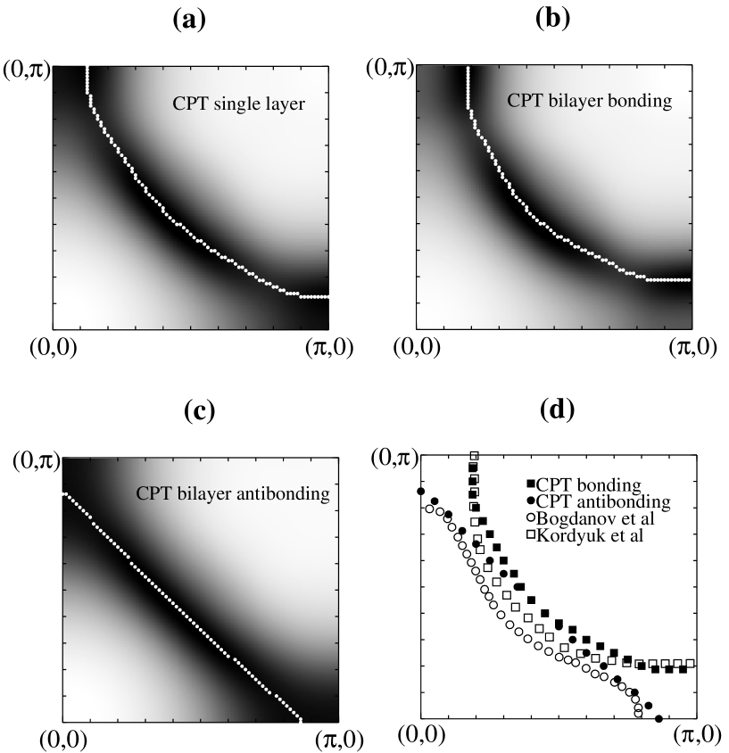
Figure 3: Spectral weight at the Fermi energy giving an estimate of the position of the Fermi surface. Results are displayed for a single CuO₂ layer (a) and for the bonding (b) and antibonding (c) band of a bilayer with interlayer hopping $t_{\perp}=0.1t_{pd}$. The white dots indicate the maxima of the spectral weight on a given branch. Panel (d) shows the comparison with experimental results on overdoped (Bi,Pb)-2212 at 22eV photon energy [35](empty squares) and and slightly overdoped (Bi,Pb)-2212 at 55eV photon energy [19](empty circles). Filled squares and circles denote the results of the CPT calculation for the bonding and antibonding branch, respectively.

We now turn to the doped systems. Here, we assume, as a first guess, that the parameters are not significantly dependent on the doping and on the particular material, and we keep the same ones for the doped region. The minimum doping that can be achieved with a 12-site cluster by adding an additional electron is $\delta=0.25$. This undoubtedly high doping is nevertheless well suited to be compared to the detailed experimental results on dispersion [20] and Fermi surface [14, 15, 16, 17, 18, 19] of the overdoped cuprates. The results of our calculation are plotted in Fig. 2. The quasiparticle dispersion from $k=(0,0)$ to $k=(\pi,\pi)$ exhibits a steep ascent beginning at a binding energy of $\sim-0.5eV$ and crossing the Fermi energy shortly before $k=(\pi/2,\pi/2)$. Starting from $k=(0,0)$ and going along (1,0), the dispersion reaches a saddle point at $\sim k=(\pi,0)$ well below the Fermi energy at $\sim-100meV$. A similar saddle-point dispersion is observed in the experimental data for Bi₂Sr₂CaCu₂O_8+δ [20], shown for comparison in the right panel of Fig. 2. The good qualitative agreement of our numerical results with the experimental ones suggests that our approach of taking the same parameter values in the undoped and in the overdoped systems is quite reasonable. This was also found earlier by intensive QMC simulation [8].

The magnitude of the spectral weight at the Fermi energy is displayed as a grayscale plot in Fig. 3 for the whole Brillouin zone. The darkest regions, thus, give an estimate of the location of the Fermi surface. The data clearly show a hole-like barrel closed around $k=(\pi,\pi)$, as usually observed in ARPES experiments on the overdoped cuprates [14, 17, 35, 36], mostly at a photon energy of $E_{\nu}\approx 22eV$. On the other hand, experiments carried out at a higher energy [15, 19, 37] $E_{\nu}=33eV$ disagree with these results, and report an electron-like Fermi surface. This is quite puzzling, and there is not yet a full consensus about this issue. Some recent papers suggest that the observation of two different Fermi surfaces is actually due to the splitting from the coupling between the bilayers [19, 16]. Nevertheless, our data suggest that, if the bilayer splitting is not relevant, the Fermi Surface should be hole-like.

The coupling between two layers can be treated without further difficulties within our method. Again, we diagonalize a $2\times 2$ unit cell exactly and include an interlayer hopping term $t_{\perp}$ within the CPT treatment. Since the effective hopping $t_{\perp}$ under consideration is relatively small and CPT amounts to a perturbation in the intercluster hopping, we believe that this is a good procedure.

The interplane hopping has been analized in studies based on LDA calculations and has been mapped on effective multi-orbital models by integrating out high-energy degrees of freedom [34]. This approach provides results which are consistent with the experimentally observed bilayer splitting [16]. In our calculation, we adopt this idea by treating the orbital phase factors of the various interplane hoppings accordingly. We take a value of $t_{\perp}\approx 0.1t_{pd}$, which is sufficient to produce an observable splitting of the Fermi surface.

Figure 3 (right panel) displays our results obtained for the bilayer. Different experimental results are shown in the last panel for comparison. Two branches can be distinguished, one being almost a square closed around $k=(\pi,\pi)$, The other one is closing around ${k=(0,0)}$, forming an electron-like Fermi surface as observed in Ref. bogd2001. Similar results have also been found by first-principle calculations of ARPES in Bi2212 [38]. These results suggests, that a possible reason for the crucial differences in the experimental observations might be found in interlayer processes. An explanation of the apparent dependence of the Fermi surface on the photon energy would require the consideration of matrix element effects which have not been addressed within this paper, but are treated in detail elsewhere [39].

4 CONCLUSION

This paper reports a systematic study of single-particle spectral properties of the three-band Hubbard model in the half-filled and in the doped region. In order to obtain sufficiently accurate results and to sort out details of the band dispersion we adopt a method (so-called CPT) combining exact diagonalization of small clusters with a perturbation in the intercluster hopping. This analysis allows us to determine a parameter set, which appropriately describes both the insulating as well as the overdoped region and gives a good agreement with ARPES data. The Fermi surface obtained at high dopings is hole like, although an interlayer hopping of about $t_{\perp}\approx 0.1t_{pd}$ produces a splitting into an electron and a hole-like Fermi surface , in agreement with ARPES experiments.

References

- [1] C. Dürr et al., Phys. Rev. B 63, 014505 (2001).
- [2] S. LaRosa et al., Phys. Rev. B 56, R525 (1997).
- [3] B. O. Wells et al., Phys. Rev. Lett. 74, 964 (1995).
- [4] F. C. Zhang and T. M. Rice, Phys. Rev. B 37, 3759 (1988).
- [5] R. Preuss, W. Hanke, and W. von der Linden, Phys. Rev. Lett. 75, 1344 (1995).
- [6] R. Eder, Y. Ohta, and G. A. Sawatzky, Phys. Rev. B 55, R3414 (1997).
- [7] G. Dopf, A. Muramatsu, and W. Hanke, Phys. Rev. B 41, 9264 (1990).
- [8] G. Dopf et al., Phys. Rev. Lett. 68, 353 (1992).
- [9] G. Dopf et al., Phys. Rev. Lett. 68, 2082 (1992).
- [10] D. Senechal, D. Perez, and M. Pioro-Ladriere, Phys. Rev. Lett. 84, 522 (2000).
- [11] M. G. Zacher et al., Phys. Rev. Lett. 85, 2585 (2000).
- [12] M. G. Zacher et al., cond-mat/0103030.
- [13] P. Fulde, Electron Correlations in Molecules and Solids (Springer, Berlin, 1995).
- [14] H. Fretwell et al., Phys. Rev. Lett. 84, 4449 (2000).
- [15] A. D. Gromko et al., cond-mat/0003017 (2000).
- [16] D. L. Feng et al., Phys. Rev. Lett. 86, 5550 (2001).
- [17] J. Mesot et al., Phys. Rev. B 63, 224516 (2001).
- [18] M. S. Golden et al., Physica C 341–348, 2099 (2000).
- [19] P. V. Bogdanov et al., cond-mat/0005394 (2000).
- [20] D. S. Marshall et al., Phys. Rev. Lett. 76, 4841 (1996).
- [21] W. Brenig, Phys. Rep. 251, 153 (1995).
- [22] Z.-X. Shen, and D. S. Dessau, Phys. Rep. 253, 1 (1995).
- [23] V. J. Emery, Phys. Rev. Lett. 58, 2794 (1987); V. J. Emery and G. Reiter Phys. Rev. B 38, 4547 (1988).
- [24] E. Arrigoni, Phys. Rev. Lett. 80, 790 (1998).
- [25] D. Boies, C. Bourbonnais, and A.-M. S. Tremblay, Phys. Rev. Lett. 74, 968 (1995).
- [26] E. Arrigoni, Phys. Rev. Lett. 83, 128 (1999).
- [27] S. Uchida et al., Phys. Rev. B 43, 7942 (1991).
- [28] S. L. Cooper et al., Phys. Rev. B 47, 8233 (1993).
- [29] M. S. Hybertsen et al., Phys. Rev. B 41, 11068 (1990).
- [30] T. Tohyama and S. Maekawa, Supercond. Sci. Technol. 13, R17 (2000).
- [31] J. M. Eroles, C. D. Batista, and A. A. Aligia, cond-mat/9812325 (1998).
- [32] F. Lema and A. A. Aligia Physica C 307, 307 (1998).
- [33] A. Damascelli, D. H. Lu, and Z. X. Shen, J. Electron Spectr. Relat. Phenom. 117–118, 165 (2001).
- [34] O. K. Andersen et al., J. Phys. Chem. Solids 56, 1573 (1995).
- [35] A. A. Kordyuk et al., cond-mat/0104294 (2001).
- [36] S. Legner et al., Phys. Rev. B 62,154 (2000).
- [37] Y. D. Chuang et al., Phys. Rev. Lett. 83, 3717 (1999).
- [38] A. Bansil and M. Lindroos, Phys. Rev. Lett. 83, 5154 (1999).
- [39] C. Dahnken and R. Eder, cond-mat/0109036.