On the connection between off-equilibrium response and statics in non disordered coarsening systems

Abstract

The connection between the out of equilibrium linear response function and static properties established by Franz, Mezard, Parisi and Peliti for slowly relaxing systems is analyzed in the context of phase ordering processes. Separating the response in the bulk of domains from interface response, we find that in order for the connection to hold the interface contribution must be asymptotically negligible. How fast this happens depends on the competition between interface curvature and the perturbing external field in driving domain growth. This competition depends on space dimensionality and there exists a critical value $d_{c}=3$ below which the interface response becomes increasingly important eventually invalidating the connection between statics and dynamics as the limit $d=1$ is reached. This mechanism is analyzed numerically for the Ising model with $d$ ranging from $1$ to $4$ and analytically for a continuous spin model with arbitrary dimensionality.

I Introduction

The off-equilibrium character of the time evolution of a system undergoing a phase ordering process, such as a ferromagnet quenched below the critical point, is clearly manifested by the aging property observed in the response function. If the system is cooled in zero field and left in the low temperature phase for a time $t_{w}$ before applying an external field, for $t_{w}$ sufficiently large the time dependent magnetization displays a behavior of the type

$$M(t,t_{w})\simeq M_{st}(t-t_{w})+M_{ag}(t,t_{w})$$ (1)

where $M_{st}(t-t_{w})$ is a stationary time translation invariant (TTI) contribution and the remaining term $M_{ag}(t,t_{w})$ is the aging contribution obeying the scaling form

$$M_{ag}(t,t_{w})=t_{w}^{-a}{\cal M}\left(\frac{t}{t_{w}}\right).$$ (2)

A structure of the same type shows up also in the autocorrelation function given by

$$C(t,t_{w})\simeq C_{st}(t-t_{w})+C_{ag}\left(\frac{t}{t_{w}}\right).$$ (3)

Behaviors like (1) and (3) are common features of slow relaxation and are the object of very intensive study especially in glassy systems, with and without disorder [1].

In the case of systems evolving via domain coarsening, structures of this type can be readily interpreted in terms of two independent variables responsible, respectively, of the fast thermal fluctuations within domains and of the slow out of equilibrium interface dynamics. The splitting of the order parameter into thermal and ordering components was used some time ago [2] as the key ingredient in the theory of phase ordering. Therefore, the stationary contributions in (1) and (3) are due to equilibrium thermal fluctuations in the bulk of domains, while the aging terms come from the remaining out of equilibrium fluctuations occurring at the passage of interfaces [3, 4].

In the study of glassy systems, along with the realization that in these systems the out of equilibrium properties are of foremost importance, recently there has been a pair of developments which have further enhanced the interest in the dynamics of slow relaxation. The first has been the off-equilibrium generalization of the fluctuation dissipation theorem (FDT), first derived by Cugliandolo and Kurchan [5] in the context of mean field models for spin glasses. This amounts to the statement that for $t_{w}\rightarrow\infty$ the magnetization depends on the time variables only through the autocorrelation function

$$M(t,t_{w})=M[C(t,t_{w})]$$ (4)

and the deviation from the ordinary FDT can be expressed through the so called fluctuation dissipation ratio (FDR)

$$X(C)=-\frac{dM(C)}{dC}$$ (5)

which obeys $X(C)=1$ in equilibrium. The second is a theorem by Franz, Mezard, Parisi and Peliti (FMPP) [6] which allows to retrieve the structure of the equilibrium state from dynamic properties during relaxation. Under certain hypothesis, they have established the identity

$$\left.\frac{dX(C)}{dC}\right]_{C=q}=P(q)$$ (6)

where $P(q)$ is the overlap probability distribution in the equilibrium state [7]. This latter development is of particular significance, since it opens a way around the difficulty of static computations for systems with complex equilibrium states.

In this context, the phase ordering process in pure systems is of considerable interest as a simplified framework where the chain of connections aging-FDR-statics can be analyzed and tested. The main point is that the phenomenology of phase ordering displays the typical features (1) and (3) of slow relaxation, and that the structure of the equilibrium state is exactly known, thus allowing for a detailed investigation of the relation between statics and dynamics. Work in this direction [3, 8, 9] has led to the conclusion that the aging term in the response function does not play any role asymptotically, therefore relegating the connection between static and dynamic properties in the somewhat trivial bulk contribution. The argument is based on the statement that interface response comes only from the spins on the border of growing domains, yielding the upper bound

$$M_{ag}(t,t_{w})\leq\rho_{I}(t_{w})\simeq L^{-1}(t_{w})$$ (7)

where $\rho_{I}(t_{w})$ is the interface density and $L(t_{w})\sim t_{w}^{1/z}$ is the typical domain size. This fits into the form (2) with $a=1/z$, where $z$ is the growth exponent.

However, this picture is at variance with exact analytical results for the one dimensional Ising model [10, 11] in the limit of infinite ferromagnetic coupling (the reason for taking this limit rather than the zero temperature limit will be discussed in Section 6). In this case one finds the opposite situation, namely there is no bulk response, while the interface response obeys (2) with $a=0$ and

$${\cal M}\left(\frac{t}{t_{w}}\right)=\frac{\sqrt{2}}{\pi}\arctan\sqrt{\frac{t}{t_{w}}-1}$$ (8)

yielding a finite asymptotic value independent of $t_{w}$

$$\lim_{t\rightarrow\infty}M_{ag}(t,t_{w})=\frac{1}{\sqrt{2}}.$$ (9)

Similarly, there is no stationary term in the autocorrelation function, while the aging term is given by [12, 13]

$$C_{ag}\left(\frac{t}{t_{w}}\right)=\frac{2}{\pi}\arcsin\left(\frac{2}{1+\frac{t}{t_{w}}}\right).$$ (10)

Hence, eliminating $t/t_{w}$ between (8) and (10) one finds (Fig. 1)

$$M(C)=\frac{\sqrt{2}}{\pi}\arctan\left[\sqrt{2}\cot\left(\frac{\pi}{2}C\right)\right]$$ (11)

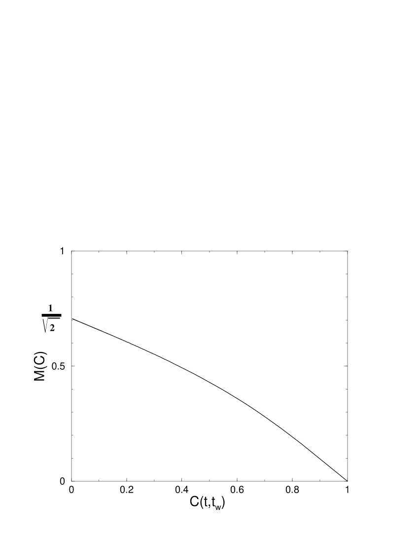
FIG. 1.: $M(C)$ for the $d=1$ Ising model with $J=\infty$.

showing that the response function obeys (4) for any $t_{w}$ giving rise to a non trivial FDR which, however, leads to a violation of the connection (6) between static and dynamic properties. This result indicates that the aging part of the response function for coarsening systems might not be as simple as (7). In order to address this problem [14], we have analyzed the behavior of the interface contribution to the response function as dimensionality is varied, finding through simulations for Ising spins and a phenomenological model for continuous spins that the interface contribution is indeed less trivial than hitherto believed. We find that the scaling form (2) holds with a scaling function and an exponent $a$ which depend on dimensionality, providing a unified coherent picture for the diverse behaviors observed at different dimensionalities. More specifically, we find that $d_{c}=3$ is the critical dimensionality such that:

i) for $d>d_{c}$ the response is actually due only to the polarization of the spins at the interfaces making (7) to hold

ii) for $d<d_{c}$ there is a new and non trivial behavior of the response function due to the competition in the motion of interfaces between the drive of the curvature, aiming to minimize surface tension, and the drive of the external field, aiming to minimize the magnetic energy of domains.

The paper is organized as follows. In Section 2 general concepts about the structure of phase space and time evolution are reviewed. Section 3 and Section 4 are devoted, respectively, to the relaxation process dominated by the fast degrees of freedom leading to equilibration and to the phase ordering process which is, conversely, dominated by the slow out of equilibrium degrees of freedom. Section 5 contains a short account of the FMPP scheme for the connection between static and dynamic properties. Section 6 and Section 7 contain results, respectively, for the Ising model in $d=1$ and in higher dimensions. The model for continuous spins is presented in Section 8 and concluding remarks are made in Section 9.

II Structure of phase space

Let us consider a spin system with hamiltonian ${\cal H}[s_{i}]$, for instance the ferromagnetic Ising model, in contact with a thermal reservoir at the temperature $T$. Below the critical temperature $T_{c}$ configuration space breaks up into ergodic components [15]

$$\Omega=\left(U_{\alpha}\Omega_{\alpha}\right)U\Omega_{b}$$ (12)

where by $\Omega_{\alpha}$, with $\alpha=\pm$ we have denoted the basins of attraction of pure states and by $\Omega_{b}$ the boundary between them [16]. The Gibbs state

$$\rho_{G}(\omega)=\frac{1}{Z}e^{-\frac{1}{T}{\cal H}(\omega)}$$ (13)

is the mixture of the two broken symmetry pure states

$$\rho_{G}(\omega)=w_{+}\rho_{+}(\omega)+w_{-}\rho_{-}(\omega)$$ (14)

where $Z=\sum_{\omega\in\Omega}e^{-\frac{1}{T}{\cal H}(\omega)}$, $\omega=[s_{i}]$ is a spin configuration, the pure states are given by

$$\rho_{\alpha}(\omega)=\left\{\begin{array}[]{ll}\frac{1}{Z_{\alpha}}e^{-\frac{1}{T}{\cal H}(\omega)}&\mbox{, if $\omega\in\Omega_{\alpha}$}\\ 0&\mbox{, if $\omega\notin\Omega_{\alpha}$}\end{array}\right.$$ (15)

and $w_{+}=w_{-}=1/2$. In each pure state there is spontaneous magnetization

$$m_{\pm}=\frac{1}{N}\sum_{i}\langle s_{i}\rangle_{\pm}=\pm m_{T}$$ (16)

and a finite correlation length $\xi_{T}$ which does not depend on the sign of the state and is related to the relaxation time within the pure state by

$$\tau^{1/z}\sim\xi_{T}.$$ (17)

In what follows $\tau$ will characterize the time scale of fast relaxation.

Alternatively, defining the overlap of two configurations by

$$Q(\omega,\omega^{\prime})=\frac{1}{N}\sum_{i}s_{i}s_{i}^{\prime}$$ (18)

the structure of a state $\rho(\omega)$ can be characterized through the probability [7] that $Q(\omega,\omega^{\prime})$ takes the value $q$ when $\omega$ and $\omega^{\prime}$ are configurations of two independent copies of the system

$$P(q)=\sum_{\omega,\omega^{\prime}}\rho(\omega)\rho(\omega^{\prime})\delta\left(Q(\omega,\omega^{\prime})-q\right).$$ (19)

Using (14) and (16), the overlap probability function in the Gibbs state is given by

$$P_{G}(q)=(w_{+}^{2}+w_{-}^{2})\delta(q-m_{T}^{2})+2w_{+}w_{-}\delta(q+m_{T}^{2})$$ (20)

where the mixed character of the state is revealed by the presence of the second $\delta$-function in the right hand side. For future reference, notice that from (19) follows

$$\int dqP(q)q=\frac{1}{N}\sum_{i}\left<s_{i}\right>^{2}.$$ (21)

Let us now consider the instantaneous quench process, where the system is initially prepared in some initial state $\rho_{0}(\omega)$ and, at the time $t=0$, is put in contact with the thermal reservoir at the temperature $T<T_{c}$. Taking $t>\tau$, the measure over $\Omega$ is given by

$$\rho(\omega,t)=\sum_{\alpha}\rho_{0}(\Omega_{\alpha})\rho_{\alpha}(\omega)+\rho_{b}(\omega,t)$$ (22)

where $\rho_{0}(\Omega_{\alpha})=\sum_{\omega\in\Omega_{\alpha}}\rho_{0}(\omega)$ and $\rho_{b}(\omega,t)$ is the measure over the boundary. Similarly, for the joint probability at times $t>t^{\prime}>\tau$ we may write

$$\rho(\omega^{\prime}t^{\prime},\omega t)=\sum_{\alpha}\rho_{0}(\Omega_{\alpha})\rho_{\alpha}(\omega^{\prime},\omega,t-t^{\prime})+\rho_{b}(\omega^{\prime}t^{\prime},\omega t)$$ (23)

where $\rho_{\alpha}(\omega^{\prime},\omega,t-t^{\prime})$ is the TTI pure state joint probability. From (22) and (23) it is quite clear that the properties of the system following a quench below $T_{c}$ are sensitive [15] to the choice of the initial condition $\rho_{0}(\omega)$, specifically to the weight given at the time $t=0$ to the different components.

At the level of the observables of interest, like magnetization $m(t)=\langle s_{i}(t)\rangle$ and correlation function $C(\mid i-j\mid,t,t^{\prime})=\langle s_{i}(t)s_{j}(t^{\prime})\rangle-\langle s_{i}(t)\rangle\langle s_{j}(t^{\prime})\rangle$, where space translation invariance is assumed to hold, the above results translate in the following way. From (22) follows that for $t>\tau$

$$m(t)=\sum_{\alpha}\rho_{0}(\Omega_{\alpha})m_{\alpha}+m_{b}(t)$$ (24)

where $m_{\alpha}$ is the equilibrium value of the magnetization in the pure states given by (16). Next, assuming that on the boundary $m_{b}(t)=0$, for $t>t^{\prime}>\tau$ and from (23) we have

$$C(\mid i-j\mid,t,t^{\prime}) = \left[\sum_{\alpha}\rho_{0}(\Omega_{\alpha})\right]C_{ps}(\mid i-j\mid,t-t^{\prime})$$ (25)

$$+ C_{b}(\mid i-j\mid,t,t^{\prime})+\Delta m$$ (26)

where

$$C_{ps}(\mid i-j\mid,t-t^{\prime})=\langle s_{i}(t)s_{j}(t^{\prime})\rangle_{\alpha}-m_{\alpha}^{2}$$ (27)

is the TTI correlation function in the equilibrium pure states which, for pure states related by symmetry, is independent of $\alpha$. Furthermore

$$C_{b}(\mid i-j\mid,t,t^{\prime})=\langle s_{i}(t)s_{j}(t^{\prime})\rangle_{b}$$ (28)

is the correlation function on the boundary and

$$\Delta m=\sum_{\alpha}\rho_{0}(\Omega_{\alpha})m_{\alpha}^{2}-\left[\sum_{\alpha}\rho_{0}(\Omega_{\alpha})m_{\alpha}\right]^{2}$$ (29)

gives the fluctuation of the magnetization over pure states. Properties of the pure state correlation function which will be needed in the following are

$$C_{ps}(\mid i-j\mid=0,t-t^{\prime}=0)=1-m_{T}^{2}$$ (30)

where we have used $s_{i}^{2}=1$, and

$$C_{ps}(\mid i-j\mid,t-t^{\prime})=0$$ (31)

for $\mid i-j\mid>\xi_{T}$ or $t-t^{\prime}>\tau$.

III Fast process: Relaxation to equilibrium

Let us now adjust the initial condition of the quench in order to have relaxation to the Gibbs state (13). From (14) and (15) the Gibbs state is the mixture of pure states with weights $w_{\alpha}=Z_{\alpha}/Z$. Hence, according to (22) relaxation to the Gibbs state can take place only if the initial condition is such that

$$\left\{\begin{array}[]{ll}\rho_{0}(\Omega_{\alpha})=\frac{Z_{\alpha}}{Z}\\ \rho_{0}(\Omega_{b})=0.\end{array}\right.$$ (32)

With such an arrangement, equilibrium is reached in the time scale $\tau$. Having now $\sum_{\alpha}\rho_{0}(\Omega_{\alpha})=1$, with $\rho_{0}(\Omega_{\alpha})=1/2$ independent of $\alpha$,  (24) and  (26) simplify to $m(t)=0$ and

$$C(|i-j|,t-t^{\prime})=C_{ps}(|i-j|,t-t^{\prime})+m_{T}^{2}$$ (33)

implying the no clustering property $C(|i-j|,t-t^{\prime})\geq m_{T}^{2}$. This behavior is illustrated in Fig. 2 depicting the autocorrelation function $C(t-t^{\prime})=C(|i-j|=0,t-t^{\prime})$ for the $d=2$ Ising model quenched to $T=0.969T_{c}$ with the initial condition $\rho_{0}(\omega)=\frac{1}{2}\delta(\omega-\omega_{+})+\frac{1}{2}\delta(\omega-\omega_{-})$ concentrating the measure on the bottom of the basins of attraction, where $\omega_{+}=[s_{i}=1,\forall i]$ and $\omega_{-}=[s_{i}=-1,\forall i]$.

FIG. 2.: Autocorrelation function for the $d=2$ Ising model with $J=1$ quenched to $T=0.969T_{c}$ ($m_{T}^{2}=0.61584$) from the initial condition $\rho_{0}(\omega)=\frac{1}{2}\delta(\omega-\omega_{+})+\frac{1}{2}\delta(\omega-\omega_{-})$ with $\omega_{+}=[s_{i}=1,\forall i]$ and $\omega_{-}=[s_{i}=-1,\forall i]$.

An observation important for what follows is that the form (33) of the correlation function corresponds to the splitting of the spin variable into the sum of two statistically independent components

$$s_{i}(t)=\psi_{i}(t)+\sigma$$ (34)

where $\psi_{i}(t)$ obeys the statistics of equilibrium thermal fluctuations in the pure state with expectations

$$\left\{\begin{array}[]{ll}\langle\psi_{i}(t)\rangle_{\alpha}=0\\ \langle\psi_{i}(t)\psi_{j}(t^{\prime})\rangle_{\alpha}=C_{ps}(|i-j|,t-t^{\prime}).\end{array}\right.$$ (35)

Instead, $\sigma$ is a time independent random variable, the ordering component, which takes the values $m_{\alpha}$ with probabilities $p(m_{\alpha})=\rho_{0}(\Omega_{\alpha})$ determined by the initial condition. Denoting the latter average by an overbar we have

$$\left\{\begin{array}[]{ll}\overline{\sigma}=0\\ \overline{\sigma^{2}}=m_{T}^{2}\end{array}\right.$$ (36)

and (33) can be rewritten as

$$C(|i-j|,t-t^{\prime})=\langle\psi_{i}(t)\psi_{j}(t^{\prime})\rangle_{\alpha}+\overline{\sigma^{2}}.$$ (37)

The next step is to study the response of the system to a perturbation. Suppose that at the time $t_{w}$ after the quench the hamiltonian ${\cal H}(\omega)$ is changed into

$${\cal H}_{h}(\omega)={\cal H}(\omega)-{\cal H}_{1}(\omega)$$ (38)

where

$${\cal H}_{1}(\omega)=\sum_{i}h_{i}s_{i}$$ (39)

is an uncorrelated gaussian random field (RF) with expectations

$$\left\{\begin{array}[]{ll}E_{h}(h_{i})=0\\ E_{h}(h_{i}h_{j})=h_{0}^{2}\delta_{ij}.\end{array}\right.$$ (40)

In the RF Ising model the lower critical dimensionality is raised from $d_{L}=1$ to $d_{L}=2$. Hence, for $d>2$ the component structure (12) of configuration space is not modified by the presence of the RF. Due to the presence of the perturbation the system will relax to a new equilibrium state

$$\rho^{*}(\omega)=\sum_{\alpha}\rho_{0}(\Omega_{\alpha})\rho_{\alpha,h}(\omega)$$ (41)

which is neither the perturbed

$$\rho_{G,h}(\omega)=\frac{1}{Z_{h}}e^{-\frac{1}{T}{\cal H}_{h}(\omega)}$$ (42)

nor the unperturbed Gibbs state (13), since the perturbation is present in the pure states, but not in the weights $\rho_{0}(\Omega_{\alpha})$. We will be interested in the linear response to the perturbation, since already in the simple context of fast relaxation it is possible to identify some of the basic elements of the connection between static and dynamic properties to be discussed in Section 5. Let us then consider the staggered magnetization defined by

$$M(t-t_{w})=\frac{T}{Nh_{0}^{2}}E_{h}\left[\langle{\cal H}_{1}(t)\rangle_{h}\right]=\frac{T}{Nh_{0}^{2}}E_{h}\left[\sum_{i}\langle s_{i}(t)\rangle_{h}h_{i}\right]$$ (43)

where $\langle\cdot\rangle_{h}$ denotes the thermal average for a given RF realization. Taking $t_{w}>\tau$, i.e. switching on the perturbation after the unperturbed system has reached equilibrium, this quantity depends only on the time difference. Since by definition $\langle\psi_{i}(t)\rangle=0$, we may write $\langle s_{i}(t)\rangle_{h}=\overline{\sigma_{i}(t)}^{h}$ where, due to the RF, the ordering component $\sigma$ acquires a site and time dependence. Expanding up to linear order in the field and recalling that the unperturbed average $\overline{\sigma}$ vanishes we have

$$\overline{\sigma_{i}(t)}^{h}=\sum_{j}\chi(|i-j|,t-t_{w})h_{j}+{\cal O}(h^{2})$$ (44)

where from (41)

$$\chi(|i-j|,t-t_{w})=\sum_{\alpha}\rho_{0}(\Omega_{\alpha})\chi_{\alpha}(|i-j|,t-t_{w})$$ (45)

and for pure states related by symmetry $\chi_{\alpha}(|i-j|,t-t_{w})$ is independent of $\alpha$. Inserting (44) and (45) into (43) we obtain

$$M(t-t_{w})=T\chi_{\alpha}(t-t_{w})$$ (46)

where $\chi_{\alpha}(t-t_{w})=\chi_{\alpha}(|i-j|=0,t-t_{w})$. Hence, $\lim_{t\to\infty}M(t-t_{w})=M_{\alpha}=T\chi_{\alpha}$ where, using (30), the static susceptibility in either one of the pure states is given by

$$\chi_{\alpha}=\frac{1}{T}\left[1-m_{T}^{2}\right].$$ (47)

This can also be rewritten as

$$M_{\alpha}=1-\int dqP_{\alpha}(q)q$$ (48)

where

$$P_{\alpha}(q)=\delta(q-m_{T}^{2})$$ (49)

is the overlap probability function of the unperturbed pure states. We call the attention here on the point that this result is different from what one obtains computing the susceptibility from the perturbed Gibbs state (42), which differs from (41) because the RF dependence enters also in the weights $w_{\alpha,h}$. In that case, in place of (47) one finds

$$\chi_{G}=\frac{1}{T}\left[1-\langle s_{i}\rangle_{G}^{2}\right]$$ (50)

where $\langle\cdot\rangle_{G}$ denotes the average over the unperturbed Gibbs state. Recalling (21), this can be rewritten as

$$\chi_{G}=\frac{1}{T}\left[1-\int dqP_{G}(q)q\right]$$ (51)

where now $P_{G}(q)$ is the overlap probability function (20) of the Gibbs state. However, the form  (50) or  (51) of the susceptibility cannot be reached dynamically. That is, by switching on the perturbation at the time $t_{w}$ after the quench, the $t\to\infty$ limit of the staggered magnetization is given by  (47) and not by  (50), which gives $\chi_{G}=1/T$ since $\langle s_{i}\rangle_{G}=0$.

Next, let us turn to the dynamical side of (46) and let us show, for pedagogical purposes, that (47) and (48) can also be obtained from a dynamical object like the linear response function

$$R(t-t^{\prime})=\left.\frac{\delta\langle s_{i}(t)\rangle}{\delta h_{i}(t^{\prime})}\right]_{h=0}$$ (52)

without resorting to knowledge of the equilibrium state. The response function $\chi_{\alpha}(t-t_{w})$ entering (46) and $R(t-t^{\prime})$ are related by

$$\chi_{\alpha}(t-t_{w})=\int_{t_{w}}^{t}dt^{\prime}R(t-t^{\prime})$$ (53)

and, given that the unperturbed system is in equilibrium, the linear response function and the pure state autocorrelation function are related by the FDT

$$R(t-t^{\prime})=\frac{1}{T}\frac{\partial C_{ps}(t-t^{\prime})}{\partial t^{\prime}}.$$ (54)

Since the constant term in (33) makes no contribution to the time derivative, we may replace $C_{ps}(t-t^{\prime})$ by the full autocorrelation function $C(t-t^{\prime})$, and inserting (54) in (53) we find

$$M(t-t_{w})=\int_{C(t-t_{w})}^{1}dq=\left[1-C(t-t_{w})\right].$$ (55)

This shows that when FDT holds the time dependence of $M$, or $\chi$, is entirely absorbed in the linear dependence on the autocorrelation function (Fig. 3).

FIG. 3.: $M(t-t_{w})$ against $C(t-t_{w})$ for the same quench as in Fig. 2. The horizontal dashed line represents the continuation of $M(C)$ into the unphysical region $C<m_{T}^{2}$.

From (55) $M(t-t_{w})$ reaches the equilibrium value (47) as $C(t-t_{w})$ reaches the lower bound $m_{T}^{2}$. Even though $C(t-t_{w})$ cannot fall below this value, we may extend the dependence of $M$ on $C$ into the unphysical region $C<m_{T}^{2}$ (horizontal dashed line in Fig. 3) by rewriting (55) as

$$M(C)=\int_{C}^{1}\theta(q-m_{T}^{2})dq$$ (56)

where $\theta$ denotes the Heaviside step function. Integrating by parts we find

$$M(C)=[1-C\theta(C-m_{T}^{2})]-\int_{C}^{1}dq\delta(q-m_{T}^{2})q$$ (57)

which yields

$$M(C)=\left\{\begin{array}[]{ll}1-C&\mbox{, for $m_{T}^{2}<C\leq 1$}\\ M_{\alpha}=1-m_{T}^{2}&\mbox{, for $C\leq m_{T}^{2}$}.\end{array}\right.$$ (58)

Taking $C=0$, from (57) we find $M_{\alpha}=1-\int_{0}^{1}dq\delta(q-m_{T}^{2})q$ recovering (48). In order to understand this result, notice that (56) can be regarded as obtained from (53) with the FDT in the modified form

$$R(t-t^{\prime})=\frac{X[C(t-t^{\prime})]}{T}\frac{\partial C(t-t^{\prime})}{\partial t^{\prime}}$$ (59)

where $X(C)=\theta(C-m_{T}^{2})$ is the FDR introduced in (5). Rewriting (57) as

$$M(C)=[1-CX(C)]-\int_{C}^{1}dq\frac{dX(q)}{dq}q$$ (60)

and taking again $C=0$ we find $M_{\alpha}=1-\int_{0}^{1}dq\frac{dX(q)}{dq}q$. Comparing with (48) then we find the relation (6) in the form

$$\left.\frac{dX(C)}{dC}\right]_{C=q}=P_{\alpha}(q)$$ (61)

showing that the piece of static information contained in $P_{\alpha}(q)$ is encoded into the relaxation properties through the FDR. Although this may seem an artificial exercise, it will turn out useful in the understanding of the connection between static and dynamic properties in the less trivial context of slow relaxation.

IV Slow relaxation: phase ordering

In the previous Section we have analyzed a quench process which yields equilibration in the Gibbs state within the time scale $\tau$. In order to achieve this the initial condition had to be chosen according to (32). Now we turn to phase ordering [17], where equilibrium is not reached within any finite time scale. We will find out that in order to have a phase ordering process the initial condition, in a sense, must be opposite to (32) with

$$\left\{\begin{array}[]{ll}\rho_{0}(\Omega_{\alpha})=0\\ \rho_{0}(\Omega_{b})=1.\end{array}\right.$$ (62)

Nonetheless, the fast equilibration process of the previous Section will turn out to dominate the short time behavior of phase ordering.

In order to assess how the phase ordering process fits in the general scheme of Section II, we relay on the behavior of the correlation function. Typically, the initial state is taken as the infinite temperature equilibrium state

$$\rho_{0}(\omega)=\prod_{i}p(s_{i})$$ (63)

with $p(s_{i})=1/2$ which yields the uniform measure $\rho_{0}(\omega)=2^{-N}$. Taking the shortest time after the quench $t^{\prime}$ sufficiently larger than $\tau$, the observed behavior of the correlation function is well represented by the sum of two contributions

$$C(|i-j|,t,t^{\prime})=C_{ps}(|i-j|,t-t^{\prime})+C_{ag}(|i-j|,t,t^{\prime})$$ (64)

where the first one is TTI and coincides with (27), while the second one displays aging through the scaling behavior [17, 18]

$$C_{ag}(|i-j|,t,t^{\prime})=m_{T}^{2}F_{ag}\left(\frac{|i-j|}{L(t^{\prime})},\frac{L(t)}{L(t^{\prime})}\right).$$ (65)

The characteristic length $L(t)$ grows with the power law $L(t)\sim t^{1/z}$ where $z=2$ for non conserved order parameter, as it will be considered in this paper. The scaling function $F_{ag}(x,y)$ has the properties

$$\left\{\begin{array}[]{ll}F_{ag}(0,1)=1\\ F_{ag}(x,1)\sim e^{-x^{2}}\quad,\quad\mbox{for $x\gg 1$}\\ F_{ag}(0,y)\sim y^{-\lambda}\quad\mbox{, for $y\gg 1$}\end{array}\right.$$ (66)

with $\lambda>0$. This shows that, contrary to the previous case, now $C(|i-j|,t,t^{\prime})$ becomes smaller than $m_{T}^{2}$ and eventually vanishes when $|i-j|$ or $t-t^{\prime}$ becomes large. This, in turn, implies that with the uniform initial state (63) condition (62) is realized, otherwise from (26) follows that it would not be possible for $C(|i-j|,t,t^{\prime})$ to vanish at large distances or large time separations. Therefore we must have

$$C(|i-j|,t,t^{\prime})=C_{b}(|i-j|,t,t^{\prime})$$ (67)

revealing that the structure (64) reflects a property of the evolution over the boundary $\Omega_{b}$. In the simplest case of the ferromagnetic system with two pure states, as we are considering, it is well known that the time evolution of configurations is given by the coarsening of domains of the two opposite equilibrium phases. Taking $t^{\prime}\gg\tau$ in order to separate the time scales of fast and slow dynamics, within each domain the system is in equilibrium in either one of the two pure states $\rho_{\pm}(\omega)$. Putting this together with (64), since in the time regime $t-t^{\prime}\ll t^{\prime}$ and for short distance $C_{ag}\simeq m_{T}^{2}$, we have that over short time and short distances the correlation function is indistinguishable from (33). Namely, we may regard the phase ordering process as a fast relaxation process of the type considered in the previous Section, followed by a quite different and much more slow relaxation taking place on the time scale set by $t^{\prime}$. This suggests the separation of the spin variable into a fast and a slow component, by generalization of the split (34) in the form [2, 4]

$$s_{i}(t)=\psi_{i}(t)+\sigma_{i}(t)$$ (68)

where, again, $\psi_{i}$ and $\sigma_{i}$ are two statistically independent variables. By analogy with  (34), we define the slow ordering component by

$$\sigma_{i}(t)=\pm m_{T}$$ (69)

according to the sign of the domain the site $i$ belongs to at the time $t$. Then, the statistics of the one time properties of $\sigma_{i}(t)$ is determined by the relative occurrence of domains of either sign, which yields the time independent probability $p(\sigma_{i})=1/2$ and the expectations

$$\left\{\begin{array}[]{ll}\overline{\sigma_{i}(t)}=0\\ \overline{\sigma_{i}^{2}(t)}=m_{T}^{2}\end{array}\right.$$ (70)

as in  (36). However, since $\sigma_{i}(t)$ changes sign whenever an interface passes through the site $i$, the two times statistics is determined by the out equilibrium interface motion. With this choice for the ordering component, $\psi_{i}$ represents the fast thermal fluctuations in the bulk of domains with the statistics of the equilibrium pure states, which is independent of the sign of domains. From  (68) then follows

$$C(|i-j|,t,t_{w})=\langle\psi_{i}(t)\psi_{j}(t_{w})\rangle_{\alpha}+\overline{\sigma_{i}(t)\sigma_{j}(t_{w})}$$ (71)

and comparing with  (64) we can make the identifications

$$\langle\psi_{i}(t)\psi_{j}(t_{w})\rangle_{\alpha}=C_{ps}(|i-j|,t-t_{w})$$ (72)

$$\overline{\sigma_{i}(t)\sigma_{j}(t_{w})}=C_{ag}(|i-j|,t,t_{w}).$$ (73)

After surveying the unperturbed phase ordering process, let us go over to the behavior of the staggered magnetization (43) after switching on the perturbation (39) at the time $t_{w}$. As mentioned above, with the RF the lower critical dimensionality is $d_{L}=2$. We will assume that the external field is so small that the bound on the size of domains imposed by the Imry Ma length $\xi(h_{0})$ for $d\leq 2$ is much larger than the size of domains $L(t)$ in the time region of interest. Therefore, we shall deal with coarsening, irrespective of dimensionality. Using the split (68) and following the argument of the previous Section we have again $\langle s_{i}(t)\rangle_{h}=\overline{\sigma_{i}(t)}^{h}$. Expanding up to linear order we generalize (44) by writing

$$\overline{\sigma_{i}(t)}^{h}=\sum_{j}\chi_{B}(|i-j|,t-t_{w})h_{j}+\chi_{I}(|i-j|,t,t_{w})h_{j}+{\cal O}(h^{2})$$ (74)

where the integrated response function has been separated into the sum of two contributions. The first one accounts for the change in the magnetization in the bulk of domains and, due to the separation of the time scales of fast and slow relaxation, is TTI. In other words, this contribution ignores the existence of interfaces and therefore under all respects is the same as the integrated response analyzed in the fast relaxation process of the previous Section, i.e. $\chi_{B}(t-t_{w})=\chi_{\alpha}(t-t_{w})$. Instead, the second contribution accounts for the extra response due to the existence of interfaces and is not TTI. Inserting in (43), in place of (46) we now have

$$M(t,t_{w})=T\chi_{B}(t-t_{w})+T\chi_{I}(t,t_{w}).$$ (75)

By definition, the bulk contribution obeys FDT and therefore, following the discussion of the previous Section, is related to the autocorrelation function by (58), with the difference that now the region $C<m_{T}^{2}$ is not unphysical.

For what concerns the interface contribution, in the first time regime with $t-t_{w}\ll t_{w}$ interfaces can be regarded as static and it is quite reasonable to take $\chi_{I}$ proportional to the interface density $\chi_{I}(t,t_{w})\simeq\rho_{I}(t_{w})\sim L^{-1}(t_{w})$. The question is what happens in the aging regime $t-t_{w}\gg t_{w}$ dominated by interface motion. The usual argument [3, 6, 9] is that $\chi_{I}$ keeps on being proportional to the interface density

$$\chi_{I}(t,t_{w})\sim\rho_{I}(t)$$ (76)

and therefore eventually disappears like $L^{-1}(t)$. If so, it is clear that by taking $t_{w}$ large enough the interface contribution can be made negligible with respect to the bulk contribution, leaving (58) to account for the relation between the whole response and the autocorrelation function. However, as explained in the Introduction and as we shall see later on, the interface response function turns out to have more structure than what (76) allows for. In particular, there is a dependence on space dimensionality which cannot be accounted for by (76).

V Statics from Dynamics

Let us now come to the problem of detecting the structure of the equilibrium state from the properties of the linear response function in the off-equilibrium regime. This requires, first of all, the generalization of FDT out of equilibrium. As we have seen in Section 3 when FDT holds the time dependence of $\chi(t-t_{w})$ is absorbed into the dependence on $C(t-t_{w})$. In the FDT generalization proposed by Cugliandolo and Kurchan [5], as stated in the Introduction, this holds also in the aging regime postulating that for large $t_{w}$

$$\chi(t,t_{w})=\chi[C(t,t_{w})].$$ (77)

In order to establish the connection between the FDR (5) and the static properties, FMPP have considered the general case in which at the time $t_{w}$ the hamiltonian is changed into ${\cal H}_{J}[s]={\cal H}_{0}[s]-{\cal H}_{p}[s]$ with a perturbation of the form ${\cal H}_{p}[s]=\sum_{i_{1}<..<i_{p}}J_{i_{1}..i_{p}}s_{i_{1}}..s_{i_{p}}$ where the couplings $J_{i_{1}..i_{p}}$ are independent gaussian variables. By considering the behavior of the expectation $E_{J}[\langle{\cal H}_{p}(t)\rangle_{J}]$ they have derived the connection between the FDR and the overlap probability function of the equilibrium state. Here, for simplicity, we reproduce the main steps of the argument in the particular case of $p=1$, when the perturbation ${\cal H}_{p}$ reduces to the form (39), referring to [6] for the treatment with arbitrary $p$.

The expectation entering in the definition of the staggered magnetization can be written as

$$E_{h}[\langle{\cal H}_{1}(t)\rangle_{h}]=E_{h}\sum_{\omega}\rho_{h}(\omega,t){\cal H}_{1}(\omega)$$ (78)

where $\rho_{h}(\omega,t)$ is the probability distribution evolving with the hamiltonian (38). Using the fact that $h_{i}$ are independent gaussian variables and integrating by parts

$$E_{h}\left[\langle{\cal H}_{1}(t)\rangle_{h}\right]=h_{0}^{2}E_{h}\left[\sum_{i}\frac{\partial}{\partial h_{i}}\left(\sum_{\omega}\rho_{h}(\omega,t)s_{i}\right)\right].$$ (79)

The same quantity can be evaluated dynamically in the Martin-Siggia-Rose formalism [6] and, assuming that (77) holds, one finds

$$E_{h}\left[\langle{\cal H}_{1}(t)\rangle_{h}\right] = \frac{h_{0}^{2}}{T}NE_{h}\Bigg{[}1-C_{h}(t,t_{w})X_{h}(C_{h}(t,t_{w}))$$ (80)

$$- \left.\int_{C_{h}(t,t_{w})}^{1}dq\frac{dX_{h}(q)}{dq}q\right]$$ (81)

where $X_{h}$ and $C_{h}$ are, respectively, the FDR and the autocorrelation function in the perturbed system. Taking the $t\rightarrow\infty$ limit and using $\lim_{t\rightarrow\infty}C_{h}(t,t_{w})=0$, from (79) and (81) follows

$$E_{h}\left[\sum_{i}\frac{\partial}{\partial h_{i}}\left<s_{i}\right>_{h,\infty}\right]=\frac{N}{T}\left[1-E_{h}\left(\int_{0}^{1}dq\frac{dX_{h}(q)}{dq}q\right)\right]$$ (82)

where $\langle\cdot\rangle_{h,\infty}$ denotes the average with the probability distribution

$$\lim_{t\rightarrow\infty}\rho_{h}(\omega,t)=\rho_{h}(\omega,\infty).$$ (83)

Therefore, what we have up to this point is that under assumption (77) there exists a relation between the susceptibility in the state (83) and the first moment of the FDR in the perturbed system. In the general case one has the same relation between the generalized susceptibility with respect to $J_{i_{1}...i_{p}}$ and the $p$-th moment of the FDR. In order to go further on, more must be known about the properties of $\rho_{h}(\omega,\infty)$. In the context considered by FMPP $\rho_{h}(\omega,\infty)$ coincides with the perturbed Gibbs state (42), from which follows

$$\frac{\partial}{\partial h_{i}}\left<s_{i}\right>_{G,h}=\frac{1}{T}\left[1-\left<s_{i}\right>_{G,h}^{2}\right].$$ (84)

Inserting this in the left hand side of (82) and using (21) one finds

$$E_{h}\int dqP_{G,h}(q)q=E_{h}\int_{0}^{1}dq\frac{dX_{h}(q)}{dq}q.$$ (85)

From this and from similar relations for the higher moments one may establish the identity $P_{G,h}(q)=\frac{d}{dq}X_{h}(q)$ which yields $\tilde{P}_{G}(q)=\frac{d}{dq}\tilde{X}(q)$ where $\tilde{P}_{G}(q)=\lim_{h\to 0}P_{G,h}(q)$ and $\tilde{X}(q)=\lim_{h\to 0}X_{h}(q)$. Eventually, after establishing under what conditions $\tilde{P}_{G}(q)$ and $\tilde{X}(q)$ may be identified, respectively, with the overlap function $P_{G}(q)$ of the unperturbed Gibbs state and with the FDR $X(q)$ of the unperturbed dynamics, one has the connection between the unperturbed statics and dynamics in the form

$$P_{G}(q)=\frac{dX(q)}{dq}.$$ (86)

Here, we call the attention on the fact that to establish (85) it is essential that (84) holds in order to use (21). Furthermore, the derivative with respect to $h_{i}$ in the left hand side of (82) acts according to how the RF enters in the asymptotic state (83). Therefore, if instead of reaching the Gibbs state (42) the asymptotic state $\rho_{h}(\omega,\infty)$ coincides with the state (41), in place of (85) one finds

$$E_{h}\int dqP_{\alpha,h}(q)q=E_{h}\int_{0}^{1}dq\frac{dX_{h}(q)}{dq}q$$ (87)

where $P_{\alpha,h}(q)$ is the overlap function of the perturbed pure state. Hence, following through the argument illustrated above, in place of (86) one concludes that the unperturbed FDR is related to the overlap function of the pure unperturbed state

$$P_{\alpha}(q)=\frac{dX(q)}{dq}.$$ (88)

In summary, the static information contained in the FDR depends on how the perturbation ${\cal H}_{p}$ enters in the asymptotic state (83). We must now see in what form the scheme applies to the phase ordering process. Suppose that the interface response function $\chi_{I}(t,t_{w})$ can be neglected in (75) for $t_{w}$ sufficiently large. Then, as explained in the previous Section, assumption (77) is verified and $M(C)$ obeys (58) leading to (61) which coincides with (88). This is confirmed by numerical simulations on the Ising model for $d\geq 2$ [8, 9] which show evidence for convergence toward the form (58) in the parametric plot of $M$ versus $C$ as $t_{w}$ becomes large. Therefore, a behavior of the type (58) is the signature that the interface contribution to the response function is negligible and the phase ordering process behaves as the fast relaxation process of Section III.

VI Ising model $d=1$

In this Section and the next one we analyze the linear response in the off-equilibrium dynamics of the Ising model beginning from the one dimensional case where analytical results are available.

The system is defined by the hamiltonian with nearest neighbor interaction ${\cal H}(\omega)=-J\sum_{i}s_{i}s_{i+1}$, where $J>0$ is the ferromagnetic coupling. From equilibrium statistical mechanics we know that the equilibrium correlation function behaves as $\langle s_{i}s_{j}\rangle_{G}=e^{-\frac{|i-j|}{\xi_{T}}}$ and the correlation length is given by $\xi_{T}=-\left[\ln\tanh\left(\frac{J}{T}\right)\right]^{-1}$. Therefore ergodicity is broken for $K=J/T=\infty$, which requires either $T=0$ for $J<\infty$ or $J=\infty$ and $T$ arbitrary. Solving dynamics with $K=\infty$, the two time correlation function obeys the form (64) where only the aging contribution (65) is present with $m^{2}_{T}=1$. The explicit form of the autocorrelation function is given by (10). The reason for the absence of the TTI contribution $C_{ps}(|i-j|,t-t^{\prime})$ is clear since with $K=\infty$ the ordering component $\sigma_{i}=\pm 1$ coincides with $s_{i}$ and $\psi_{i}$ in (68) vanishes identically. Namely, in the quench with $K=\infty$ domains are formed, phase space motion takes place over $\Omega_{b}$, as demonstrated by the aging behavior of the correlation function, but thermal fluctuations are absent within domains leading to the absence of the TTI contribution in the autocorrelation function.

It is interesting to consider also what happens in the quench with $K<\infty$. In this case there is no ergodicity breaking. Solving dynamics one finds the generalized scaling form [12] $C(|i-j|,t,t^{\prime})=F\left(\frac{|i-j|}{L(t^{\prime})},\frac{L(t)}{L(t^{\prime})},\frac{L(t^{\prime})}{\xi_{T}}\right)$ with the limiting behaviors

$$F \left(\frac{|i-j|}{L(t^{\prime})},\frac{L(t)}{L(t^{\prime})},\frac{L(t^{\prime})}{\xi_{T}}\right)=$$ (92)

$$\left\{\begin{array}[]{ll}F_{st}\left(\frac{|i-j|}{\xi_{T}},\frac{t-t^{\prime}}{\tau}\right)&\mbox{, \quad for $\frac{t^{\prime}}{\tau}\gg 1$}\\ F_{ag}\left(\frac{|i-j|}{L(t^{\prime})},\frac{L(t)}{L(t^{\prime})}\right)&\mbox{, \quad for $\frac{t-t^{\prime}}{\tau}\ll 1$ and $\frac{t^{\prime}}{\tau}\ll 1$}\end{array}\right.$$

where the equilibration time $\tau$ is defined by (17) with $z=2$. The meaning of (92) is, first of all, that after a finite time $\tau$ equilibrium is reached. Hence, taking $t^{\prime}/\tau>1$ one observes the TTI behavior pertaining to the stationary dynamics in the equilibrium state. However, if $\tau$ although finite is sufficiently large to allow for $t/\tau\ll 1$, then in the time regime $(t-t^{\prime})\ll\tau$ one observes the same behavior as in the $K=\infty$ case. This can be understood considering that for $K$ large $\tau\sim e^{4K}$ is the characteristic time needed to overturn one spin originally aligned with both of its neighbors. Then, taking $t^{\prime}\ll\tau$ means that one starts to look into the system when domains are still much smaller than $\xi_{T}$. Immediately after and as long as $t<\tau$ growth continues as in the $K=\infty$ case, i.e. without thermal fluctuations within domains. Thermal fluctuations do come into play only for $t\geq\tau$. When this happens, the creation of defects by thermal fluctuations balances the losses due to interface annihilation and leads to a halt in domain growth and to the establishment of thermal equilibrium.

Let us see what happens upon applying the RF at the time $t_{w}>0$. Recall that the master equation for the system evolving with the Glauber spin flip dynamics is given by

$$\frac{\partial\rho\left(\omega,t\right)}{\partial t}=\sum_{i}\left[w(-s_{i})\rho\left(R_{i}\omega,t\right)-w(s_{i})\rho\left(\omega,t\right)\right]$$ (93)

where $R_{i}\omega$ is the configuration $\omega$ with the $i$-th spin reversed and $w(s_{i})$ is the transition rate from $\omega$ to $R_{i}\omega$ given by

$$w(s_{i})=\frac{1}{2}(1-H^{int}_{i}s_{i})(1-H^{ext}_{i}s_{i})$$ (94)

where $H^{int}_{i}=\frac{\gamma}{2}(s_{i-1}+s_{i+1})$, $H^{ext}_{i}=\tanh\left(\frac{h_{i}}{T}\right)$ and $\gamma=\tanh(2K)$. Taking $K=\infty$, let us first consider the behavior of (94) before switching on the external field, in the interval $0<t<t_{w}$. Since $\gamma=1$, we have $H^{int}_{i}=1$ if $s_{i-1}s_{i+1}=1$ and $H^{int}_{i}=0$ if $s_{i-1}s_{i+1}=-1$. In the latter case the spin $s_{i}$ is at the interface between two domains of opposite sign with probability $1/2$ per unit time to flip or not to flip. Conversely, in the former case the spin flips with probability 1 if it is not aligned with its neighbors, while it does not flip with probability 1 in the opposite case, when it belongs to the bulk of a domain. As a consequence the only dynamics in the system is the unbiased random walk of interfaces, leading to the growth law $L(t)\sim t^{1/2}$.

After switching on the RF we are interested in the behavior of the staggered magnetization (43), which is now convenient to regard as the correlation function between the external field and magnetization. Right at the start $M(t_{w},t_{w})=0$, since at $t=t_{w}$ the RF and configurations are uncorrelated. However, for $t>t_{w}$ the transition rate (94) is modified by the factor involving $H^{ext}_{i}$ which introduces a bias in the flips at the interfaces in favor of the local field, while bulk flips remain forbidden. Accordingly, $M(t,t_{w})$ grows positive revealing that spin configurations tend to correlate with the field. However, a substantial difference arises in the two ways to produce the limit $K=\infty$. If $J<\infty$ and $T=0$, $M(t,t_{w})$ rises from zero to a plateau value $\widetilde{M}$ (Fig. 4) within a microscopic time $t_{0}$ and $\widetilde{M}$ depends on $t_{w}$ according to (inset of Fig. 4)

$$\widetilde{M}(t_{w})\sim L^{-1}(t_{w}).$$ (95)

FIG. 4.: $M(t,t_{w})$ for the $d=1$ Ising model with $J=1$ quenched to $T=0$ for different waiting times ($10,10^{2},3.16\cdot 10^{2},10^{3},3.162\cdot 10^{3},10^{4},3.162\cdot 10^{4},10^{5}$ from top to bottom). In the inset, the plateau value $\widetilde{M}(t_{w})$ is plotted against $t_{w}$. The solid line is the $t_{w}^{-1/2}$ behavior.

The reason for this is that after switching on the field the motion of interfaces continues for a short time until pinning takes place when the two opposite spins making up the defect at the interface fall into a defect of the same sign in the field configuration. At that point, since $H^{ext}_{i}=\mbox{sign}\,h_{i}$, the second factor in the right hand side of (94) vanishes and the interface does not move anymore. This explains reaching the plateau and the dependence (95) of $\widetilde{M}$ on $t_{w}$, since the contribution to the staggered magnetization comes only from the spins at the interfaces and goes like the interface density. Furthermore, since $T=0$ implies $h_{0}/T=\infty$ there is no way to access the linear response regime, no matter how small the external field is chosen. Conversely, if the $K=\infty$ limit is obtained taking $J=\infty$ and with no restrictions on the temperature, while the unperturbed dynamics remains the same, interesting behavior is obtained with RF since i) $T>0$ allows to overcome pinning of the interfaces letting also the bulk of domains to participate in the correlation of spin configurations with the RF and ii) the condition $h_{0}/T\ll 1$ can be realized making accessible the linear response regime.

In the following we will concentrate in the linear response regime with $J=\infty$ and $h_{0}/T\ll 1$. In this case the staggered magnetization is given by (8). The first observation, comparing with the general form (75), is that the TTI bulk contribution is missing, as expected from the above discussion on the absence of thermal fluctuations when $K=\infty$. Hence, the result (8) is entirely due to the second contribution in (75), which however is totally different from the behavior (76) which one would expect on the basis of a straightforward interface contribution. Rather than decreasing at large time, here $M(t,t_{w})$ displays a correlation of the spin configurations with the RF which grows with time, until reaching the finite limit (9) as $t\rightarrow\infty$ (Fig. 1). Having excluded a correlation effect due to thermal fluctuations or to spin polarization at the interfaces, the increase in the correlation can only be due to the fact that interface motion is driven by the field. As we shall now see, the field driven mechanism, without modifying the growth law $L(t)\sim t^{1/2}$, induces large scale domain drift in order to optimize the position of the bulk of domains with respect to the RF configuration. It must be stressed that although involving the bulk of domains, this contribution to the staggered magnetization has nothing to do with the bulk response function coming from thermal fluctuations, which are now absent.

An insight on how the field driven mechanism works comes from the behavior of (8) for $t-t_{w}\ll t_{w}$ from which we find

$$\chi_{I}(t,t_{w})=\frac{1}{T\pi}\left[\frac{2(t-t_{w})}{t_{w}}\right]^{\frac{1}{2}}.$$ (96)

Since in this time regime the system can be regarded as a set of non interacting interfaces and the density of interfaces $\rho_{I}(t)$ at the time $t\simeq t_{w}$ is given by $L^{-1}(t_{w})$, we can rewrite (96) in the form

$$\chi_{I}(t,t_{w})=\rho_{I}(t)\chi_{eff}(t,t_{w})$$ (97)

where

$$\chi_{eff}(t,t_{w})\sim(t-t_{w})^{\frac{1}{2}}$$ (98)

is the effective response associated to a single interface. Looking next to the large time behavior for $t-t_{w}\gg t_{w}$, from (8) follows $T\chi_{I}(t,t_{w})=1/\sqrt{2}-{\cal O}(t/t_{w})^{-1/2}$ which implies that the effective single interface response follows the behavior (98) also for large time.

In order to check on this interpretation we have computed analytically the behavior of $\chi_{I}(t,t_{w})$ when in the system there is a single interface. This is done by preparing the system at $t=0$ in a configuration $\omega$ containing only one interface at the origin, for instance taking $s_{i}=1$ for $i\leq 0$ and $s_{i}=-1$ for $i>0$. The computation of the response function can be carried out exactly (see Appendix A) yielding

$$\chi_{sing}(t-t_{w})\sim(t-t_{w})^{\frac{1}{2}}$$ (99)

which substantiates the above analysis. This unexpected result makes it clear that the interface response is not simply due to the polarization of the paramagnetic interfacial spins, but is a much more complex effect. At a generic time $t$ the interface has explored a region of order $(t-t_{w})^{1/2}$ and energy can only be released by reducing the contribution to ${\cal H}_{1}(\omega)$ coming from the visited region. This can be achieved if the interface motion produces a large scale optimization of the position of domains with respect to the random field.

In summary, from the analysis of the linear response function in the quench of the $d=1$ Ising model with $K=\infty$, we have uncovered a new and non trivial behavior different from the pattern outlined in Section IV, which is the one usually expected for coarsening systems. The role of the bulk and interface terms in (75) is reversed, the response being dominated by the latter one with all the new features illustrated above.

VII Ising model $D>1$

As stated in Section 4, for the Ising model in two and three dimensions there is numerical evidence that as $t_{w}$ becomes large the staggered magnetization displays the structure  (58). For this to happen, the interface contribution in (75) must vanish and only the bulk contribution must be left over. However, the exact analysis of the previous Section in the one dimensional case is a serious warning that the interface contribution might not disappear so easily as the argument (76) could make believe. Therefore, a careful analysis of the interface contribution is needed to find out whether the field driven mechanism of interface motion is at work also in higher space dimensions. In order to do so it is necessary to give an anambiguous definition of which degrees of feedom must be cosidered interfacial. In particular, it is necessary to make clear whether the flip of a spin in the interior of a domain belongs to a bulk fluctuation or makes a new interface. The definition we adopt is the following. Consider two configurations $\omega_{I+B}$ and $\omega_{I}$ evolving from the same initial condition with the same thermal history, under the influence of the same external field, if present. While $\omega_{I+B}$ evolves with the usual Glauber dynamics, $\omega_{I}$ is subjected to the restriction that flips of bulk spins are forbidden. A bulk spin is defined as being aligned with all its nearest neighbours. Then, all the spins surrounding topological defects in $\omega_{I}$ are considered interfacial spins. On the other hand $\omega_{I+B}$ contains defects which can be either associated to interfaces or to bulk fluctuations, the latter being determined by comparison with $\omega_{I}$. On the basis of this definition we have measured the interface response function $\chi_{I}(t,t_{w})$ by simulating the evolution of the ferromagnetic Ising model with nearest neighbor interaction for $d=1,2,3,4$ without bulk flips and starting from the high temperature uncorrelated initial condition (63). We have included the simulation of the $d=1$ case, for which the exact analytical results of the previous Section are available, in order to have a check on the numerical procedure.

For the effective response associated to a single interface $\chi_{eff}(t,t_{w})$ defined by (97), we have obtained (Fig. 5) the asymptotic behavior

$$\chi_{eff}(t,t_{w})\sim(t-t_{w})^{\alpha}$$ (100)

where the numerical values of $\alpha$ are consistent with

$$\alpha=\left\{\begin{array}[]{ll}\frac{3-d}{4}&\mbox{for $d<3$}\\ 0&\mbox{for $d>3$}.\end{array}\right.$$ (101)

For $d=3$ a power law fit yields $\alpha=0.03$. A fit of the same quality is obtained with the logarithmic form $T\chi_{eff}(t,t_{w})=0.33+0.066\cdot log(t-t_{w})$.

FIG. 5.: $\chi_{eff}(t,t_{w})$ in the Ising model without spin flips in the bulk. For $d=1,2,3,4$, the temperature, waiting time and linear system size of the simulations are $T=0.48,2.2,3.3,4.4$, $t_{w}=10^{3},10^{3},10^{2},10$ and $L=10^{6},512,200,42$ with $J=1$ and averages over $170,6045,114,922$ realizations. The dashed lines are power laws with the corresponding exponent $\alpha$. For $d=3$ the curve is well fitted by $T\chi_{eff}(t,t_{w})=0.33+0.066\cdot log(t-t_{w})$.

In order to check to what extent $\chi_{eff}(t,t_{w})$ is related to a single interface response, we have performed another set of simulations without flips in the bulk, starting with an initial condition containing one straight spanning interface in the middle of the system. The results of simulations are shown in Fig. 6 and indeed the data reproduce quite well the behavior of $\chi_{eff}(t,t_{w})$, except for $d=3$. In this case the logarithmic behavior found for $\chi_{eff}(t,t_{w})$ is followed up to a certain time, beyond which the response speeds up considerably. The analysis of this behavior, for which we do not have an adequate explanation, requires numerical investigation at much larger times and goes beyond the scope of the present work.

FIG. 6.: The single interface response, obtained from simulations without flips in the bulk and with an initial condition containing one single flat interface. For $d=1,2,3,4$ temperatures of the simulations are $T=0.48,2.2,3.3,4.4$, with $J=1$, $t_{w}=0$ and averages over $151600,19810,69891,3537$ realizations. The dashed lines are power laws with the corresponding exponent $\alpha$.

In summary, comparing Fig. 5 with Fig. 6, the identification of $\chi_{eff}(t,t_{w})$ with the response associated to a single interface $\chi_{sing}(t,t_{w})$ is on the whole well founded. We must now extract the meaning of the overall behavior as dimensionality is varied. The main feature is that the power law growth (100) weakens as $d$ rises from $d=1$ to $d=3$ and disappears above $d=3$. The explanation of this behavior can be conjectured recalling that in the unperturbed system interfaces perform an unbiased random walk in $d=1$, while are curvature driven for $d\geq 2$. In the perturbed system in $d=1$, as we have seen in the previous Section, interfaces are field driven. This mechanism operates also in higher dimensions, except that it enters in competition with the curvature mechanism. The effect of the curvature becomes comparatively more important as $d$ increases due to the increasing coordination number. According to our simulations $d_{c}=3$ is the critical value of the dimensionality, such that for $d>d_{c}$ the field driven mechanism is ineffective and interface motion is dominated by the curvature yielding $\alpha=0$. Therefore, for $d>d_{c}$, interfaces respond only through the polarization of the interfacial spins. This response saturates to the asymptotic value over a microscopic time scale (curves for $d=4$ in Fig.5 and Fig.6). Conversely, for $d<d_{c}$, the field driven mechanism competes with the curvature yielding $\alpha>0$ and this competition gets more effective as dimensionality is lowered. Finally, as the limit $d=1$ is reached from above, the curvature mechanism disappears and the effectiveness of the field driven mechanism becomes complete yielding $\alpha=1/2$.

VIII Continuous spin model

The discussion of the previous Section makes clear that dimensionality plays a crucial role in determining the relative importance of the bulk and interface response. In order to clarify further this point, in this Section we present an analytical calculation of $\chi_{I}(t,t_{w})$ in the framework of continuous spins which allows to vary dimensionality freely. The approximations involved in what follows are too crude for an accurate quantitative reproduction of the results of the simulations. Nonetheless, even in this form, the continuous model is quite useful to capture the overall qualitative picture.

The treatment of phase ordering with a continuous, scalar and non conserved order parameter $\phi(\vec{x},t)$ is usually based [17] on the time dependent Ginzburg-Landau equation

$$\frac{\partial\phi}{\partial t}=\nabla^{2}\phi+r\phi-g\phi^{3}+\eta(\vec{x},t)$$ (102)

where $r$ and $g$ are positive constants and $\eta(\vec{x},t)$ is a gaussian white noise with expectations

$$\left\{\begin{array}[]{ll}\langle\eta(\vec{x},t)\rangle=0\\ \langle\eta(\vec{x}^{\prime},t^{\prime})\eta(\vec{x},t)\rangle=2T\delta(t-t^{\prime})\delta(\vec{x}-\vec{x}^{\prime}).\end{array}\right.$$ (103)

The infinite temperature initial condition is imposed taking $\phi_{0}(\vec{x})=\phi(\vec{x},t=0)$ as an additional source of noise gaussianly distributed with expectations

$$\left\{\begin{array}[]{ll}\overline{\phi_{0}(\vec{x})}=0\\ \overline{\phi_{0}(\vec{x})\phi_{0}(\vec{x}^{\prime})}=\Delta\delta(\vec{x}-\vec{x}^{\prime}).\end{array}\right.$$ (104)

In past work on phase ordering kinetics most of the effort has been devoted to the study of the scaling properties of the equal time correlation function, that is, in the present language, to the study of $C_{ag}(\mid i-j\mid,t=t^{\prime})$ in (64) and (65). For this purpose, thermal fluctuations are usually neglected eliminating the thermal noise in (102). Then, one deals with the equation

$$\frac{\partial\phi}{\partial t}=\nabla^{2}\phi+r\phi-g\phi^{3}$$ (105)

where the only source of noise is the initial condition $\phi_{0}(\vec{x})$.

From the analytical point of view, one of the most successful tools of investigation of this problem has been the gaussian auxiliary field (GAF) approximation which goes back to the pioneering work of Ohta, Jasnow and Kawasaki [19, 17]. The method is suited to study the late stage, after local equilibrium within domains has been achieved. In the case of Eq. (105) this means that locally the order parameter must sit at the bottom of either one of the two degenerate minima of the potential satisfying

$$\phi(\vec{x},t)=\pm m_{0}$$ (106)

where $m_{0}=\sqrt{r/g}$ is the $T=0$ equilibrium value of the order parameter. The idea at the basis of the GAF approximation is that (106) can be implemented through a non linear transformation on an auxiliary field $u(\vec{x},t)$ over which perturbative methods can be applied. Different versions of the approximation correspond to different realizations of the non linear transformation. Here we take the transformation of the Kawasaki, Yalabik and Gunton [20] type

$$\phi(\vec{x},t)=\frac{u(\vec{x},t)}{\sqrt{1+\frac{u^{2}(\vec{x},t)}{m_{0}^{2}}}}.$$ (107)

Then, if the non linearity of $u(\vec{x},t)$ is mild, unbounded growth is allowed eventually yielding $\phi(\vec{x},t)=m_{0}sign[u(\vec{x},t)]$ which enforces the requirement (106). In order to actually carry out computations, one has to solve the dynamics of $u(\vec{x},t)$ induced by (105) via (107), as we shall do below.

After this brief survey of the GAF method, let us go back to the equation of motion (102) including thermal fluctuations. A systematic treatment of this problem based on the Martin-Siggia-Rose formalism and on the split of the order parameter into ordering and fluctuating components was worked out in Ref. [2]. Here, we follow the same idea working directly with the equation of motion. Let us split the order parameter as in (68)

$$\phi(\vec{x},t)=\psi(\vec{x},t)+\sigma(\vec{x},t)$$ (108)

with the aim of separating the fast thermal fluctuations from the slow ordering component. Inserting (108) in (102) we find

$$\frac{\partial\psi}{\partial t}+\frac{\partial\sigma}{\partial t} = \nabla^{2}\psi+\nabla^{2}\sigma+r\psi+r\sigma-g\psi^{3}-$$ (110)

$$3g\psi^{2}\sigma-3g\psi\sigma^{2}-3g\sigma^{3}+\eta$$

and let us decouple $\psi$ from $\sigma$ replacing the mixed terms by $3g\psi^{2}\sigma\rightarrow 3g\langle\psi^{2}\rangle\sigma$ and $3g\psi\sigma^{2}\rightarrow 3g\psi\overline{\sigma^{2}}$. Furthermore, let us assume that $T$ is sufficiently lower than $T_{c}$ to justify the self-consistent linearization $\psi^{3}\rightarrow 3\langle\psi^{2}\rangle\psi$. Stipulating that $\psi$ is driven by the thermal noise and that $\sigma$ is driven by the noise in the initial condition, we obtain the pair of equations

$$\frac{\partial\psi}{\partial t}=\nabla^{2}\psi+\left[r-3g\langle\psi^{2}(\vec{x},t)\rangle-3g\overline{\sigma^{2}(\vec{x},t)}\right]\psi+\eta$$ (111)

and

$$\frac{\partial\sigma}{\partial t}=\nabla^{2}\sigma+\left[r-3g\langle\psi^{2}(\vec{x},t)\rangle\right]\sigma-g\sigma^{3}$$ (112)

with the initial conditions $\psi(\vec{x},t=0)=0$ and $\sigma(\vec{x},t=0)=\phi_{0}(\vec{x})$. Let us make the assumption, to be verified a posteriori, that $\psi$ is the fast variable with relaxation time $\tau$. Defining $r_{eq}=r-3g\langle\psi^{2}\rangle_{eq}$ and making the additional assumption that within the same time scale $\sigma(\vec{x},t)$ reaches local equilibrium with $\overline{\sigma^{2}(\vec{x},t)}=m^{2}_{T}=\frac{r_{eq}}{g}$, for $t>\tau$ in place of (111) and (112) we may write

$$\frac{\partial\psi}{\partial t} = \nabla^{2}\psi-\xi_{T}^{-2}\psi+\eta(\vec{x},t)$$ (113)

$$\frac{\partial\sigma}{\partial t} = \nabla^{2}\sigma+r_{eq}\sigma-g\sigma^{3}$$ (114)

where the equilibrium correlation length $\xi_{T}$ is given by

$$\xi_{T}^{-2}=2r_{eq}.$$ (115)

From (108) follows that the autocorrelation function is given by the sum of two contributions as in (64) $C(t,t^{\prime})=C_{ps}(t-t^{\prime})+C_{ag}(t,t^{\prime})$ with the TTI piece

$$C_{ps}(t-t^{\prime})=\langle\psi(\vec{x},t)\psi(\vec{x},t^{\prime})\rangle=\langle\psi^{2}(\vec{x})\rangle_{eq}e^{-\frac{t-t^{\prime}}{\xi_{T}^{2}}}$$ (116)

and the aging contribution

$$C_{ag}(t,t^{\prime})=\overline{\sigma(\vec{x},t)\sigma(\vec{x},t^{\prime})}.$$ (117)

The latter one can be computed from (114) using the GAF approximation with the non linear transformation of the type (107) in which $m_{0}^{2}$ is replaced by $m^{2}_{T}$

$$\sigma(\vec{x},t)=\frac{u(\vec{x},t)}{\sqrt{1+\frac{u^{2}(\vec{x},t)}{m_{T}^{2}}}}.$$ (118)

From (116) indeed follows that $\psi(\vec{x},t)$ describes the fast equilibrating thermal fluctuations with the characteristic time $\tau=\xi^{2}_{T}$.

Consider, next, the effect on the ordering component of an RF with expectations analogue to (40)

$$\left\{\begin{array}[]{ll}E_{h}[h(\vec{x})]=0\\ E_{h}[h(\vec{x})h(\vec{x}^{\prime})]=h_{0}^{2}\delta(\vec{x}-\vec{x}^{\prime}).\end{array}\right.$$ (119)

For $t>t_{w}$ the equation of motion (114) is modified into

$$\frac{\partial\sigma}{\partial t}=\nabla^{2}\sigma+r_{eq}\sigma-g\sigma^{3}+h(\vec{x})$$ (120)

while (113) for $\psi(\vec{x},t)$ remains unaltered. In order to generalize the GAF approximation, notice that the external field affects the transformation (118) in two ways: i) through the auxiliary field $u(\vec{x},t)$ and ii) by shifting the saturation value $\pm m_{T}$ of domains. Therefore, we separate a bulk and an interface term writing $\sigma(\vec{x},t)=\sigma_{B}(\vec{x},t)+\sigma_{I}(\vec{x},t)$ where

$$\sigma_{B}(\vec{x},t)=\int d\vec{x}^{\prime}\chi_{B}(\vec{x}-\vec{x}^{\prime},t-t_{w})h(\vec{x}^{\prime})$$ (121)

and

$$\sigma_{I}(\vec{x},t)=\frac{u_{h}(\vec{x},t)}{\sqrt{1+\frac{u_{h}^{2}(\vec{x},t)}{m^{2}_{T}}}}.$$ (122)

The latter one is constructed to account only for the effect of the external field on the interface motion, by keeping the saturation value at the unperturbed level $\pm m_{T}$, while the former takes care of the remaining perturbation on the bulk of domains. Hence, for the staggered magnetization the decomposition (75) applies where, according to the discussion of Section IV, $\chi_{B}$ obeys FDT and is therefore related to the autocorrelation function by (58). Here we are interested in the interface contribution

$$\chi_{I}(t,t_{w})=\frac{1}{h_{0}^{2}}E_{h}\left[\overline{\sigma_{I}(\vec{x},t)}h(\vec{x})\right]$$ (123)

and in order to compute this quantity let us go back to (120). Since we want to extract the dependence of $u_{h}(\vec{x},t)$ on the RF up to first order, after substituting $\sigma=\sigma_{B}+\sigma_{I}$ and keeping into account that $\sigma_{B}$ is a first order quantity we obtain

$$\frac{\partial\sigma_{I}}{\partial t}=\nabla^{2}\sigma_{I}+r_{eq}\sigma_{I}-g\sigma^{3}_{I}+h(\vec{x})$$ (124)

where the effect of $\sigma_{B}$ goes into a redefinition of the variance $h_{0}^{2}$ of the RF, which will be neglected in the following. Substituting (122) for $\sigma_{I}(\vec{x},t)$ and dropping the subscripts $h$, the equation of motion for the auxiliary field is given by

$$\frac{\partial u}{\partial t}=\nabla^{2}u+r_{eq}u+\frac{\sigma^{\prime\prime}(u)}{\sigma^{\prime}(u)}\left(\nabla u\right)^{2}+\frac{h(\vec{x})}{\sigma^{\prime}(u)}$$ (125)

where

$$\sigma^{\prime}(u)=\left[1+\frac{u^{2}}{m^{2}_{T}}\right]^{-\frac{3}{2}}$$ (126)

and

$$\sigma^{\prime\prime}(u)=-3\frac{u}{m_{T}^{2}}\left[1+\frac{u^{2}}{m^{2}_{T}}\right]^{-\frac{5}{2}}.$$ (127)

Performing, next, a mean field approximation by keeping only the lowest order non linear contribution in each term and linearizing self-consistently, after Fourier transforming over space we find

$$\frac{\partial u(\vec{k},t)}{\partial t}=-[k^{2}+D(t)]u(\vec{k},t)+h(\vec{k})$$ (128)

where

$$D(t)=-r_{eq}+\frac{3}{m^{2}_{T}}\overline{(\nabla u)^{2}}.$$ (129)

Defining the linear response function by

$$R(\vec{k},t,t^{\prime})=\frac{Y(t^{\prime},0)}{Y(t,0)}e^{-k^{2}(t-t^{\prime})}$$ (130)

with

$$Y(t,0)=e^{\int_{0}^{t}dsD(s)}$$ (131)

the formal solution of (128) reads

$$u(\vec{k},t)=R(\vec{k},t,0)u(\vec{k},0)+\chi_{u}(\vec{k},t,t_{w})h(\vec{k})$$ (132)

where $\chi_{u}(\vec{k},t,t_{w})=\int_{t_{w}}^{t}dt^{\prime}R(\vec{k},t,t^{\prime})$ is the integrated response function of the auxiliary field. Carrying out the self-consistent computation of $D(t)$ (Appendix B), the large time behavior of $Y(t,0)$ is given by $Y(t,0)=$

$a\left(t+\frac{1}{2\Lambda^{2}}\right)^{-\frac{d+2}{4}}$ where $\Lambda$ is a momentum cutoff and $a=\left[\frac{3\Delta d}{4r_{eq}m^{2}_{T}(8\pi)^{\frac{d}{2}}}\right]^{\frac{1}{2}}$. Inserting in (130), from $\chi_{u}(t,t_{w})=$
$(2\pi)^{-d}\int d\vec{k}\chi_{u}(\vec{k},t,t_{w})$ and $t_{w}\gg 1/\Lambda^{2}$ follows

$$\chi_{u}(t,t_{w})=(4\pi)^{-\frac{d}{2}}t^{\frac{d+2}{4}}\int_{t_{w}}^{t}dt^{\prime}t^{\prime-\frac{d+2}{4}}\left(t-t^{\prime}+\frac{1}{\Lambda^{2}}\right)^{-\frac{d}{2}}.$$ (133)

Similarly, for the unperturbed autocorrelation function of the $u$ field we find (Appendix B)

$$\overline{u(\vec{x},t)u(\vec{x},t^{\prime})}=\frac{\Delta\left[\left(t+\frac{1}{2\Lambda^{2}}\right)\left(t^{\prime}+\frac{1}{2\Lambda^{2}}\right)\right]^{\frac{d+2}{4}}}{a^{2}(4\pi)^{d/2}\left(t+t^{\prime}+\frac{1}{\Lambda^{2}}\right)^{d/2}}.$$ (134)

Now, in order to compute (123) we make a further mean field approximation by replacing (122) with

$$\sigma_{I}(\vec{x},t)=m_{T}\frac{u_{h}(\vec{x},t)}{\sqrt{S(t)}}$$ (135)

where $S(t)=\overline{u^{2}(\vec{x},t)}$ is an unperturbed average. This gives

$$\chi_{I}(t,t_{w})=\frac{m_{T}}{\sqrt{S(t)}}\chi_{u}(t,t_{w})$$ (136)

and computing $S(t)$ from (134) we get

$$S(t)=b\left(t+\frac{1}{2\Lambda^{2}}\right)$$ (137)

with $b=\frac{4r_{eq}m_{T}^{2}}{3d}$ and

$$\chi_{I}(t,t_{w})=At^{\frac{1-d}{2}}F\left(\frac{t_{w}}{t},\frac{t_{0}}{t}\right)$$ (138)

where

$$F\left(\frac{t_{w}}{t},\frac{t_{0}}{t}\right)=\int_{\frac{t_{w}}{t}}^{1}dxx^{-\frac{d+2}{4}}\left(1+\frac{t_{0}}{t}-x\right)^{-\frac{d}{2}}.$$ (139)

Here, $t_{0}=\Lambda^{-2}$ is a microscopic time and $A=\left[\frac{3d}{4r_{eq}(4\pi)^{d}}\right]^{\frac{1}{2}}$.

Next, we may use the form (135) of the transformation to compute also the aging contribution (117) to the autocorrelation function obtaining (Appendix B)

$$C_{ag}(t/t_{w})=m_{T}^{2}\left(\frac{t_{w}}{t}\right)^{d/4}\left(\frac{1}{2}+\frac{t_{w}}{2t}\right)^{-d/2}.$$ (140)

For $d=1$ the time ratio $t_{w}/t$ can be eliminated between (138) and (140) yielding a parametric plot (Fig. 7) of the response function versus $C$ qualitatively similar to the one of the $d=1$ Ising model in Fig. 1. In particular, in the large time limit we find the counterpart of (9)

$$\lim_{t\rightarrow\infty}\chi_{I}(t,t_{w})=AF(0,0)=\sqrt{\frac{3}{2r_{eq}}}\left[\frac{\Gamma(1/4)}{2\pi}\right]^{2}.$$ (141)

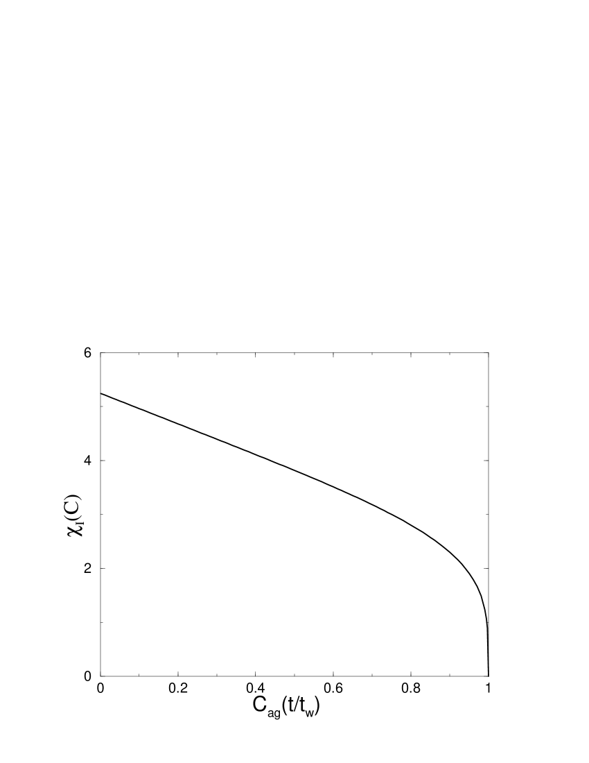
FIG. 7.: Parametric plot of $\chi_{I}$ against $C_{ag}$ in the continuous spin model.

The interesting point now is to extract the behavior of the effective response function $\chi_{eff}$ associated to the single interface and defined by (97). In the short time regime $t-t_{w}\ll t_{w}$ from (138) follows

$$\chi_{eff}(t-t_{w})=\frac{2\Lambda^{d-2}}{2-d}\left[\left(\frac{t-t_{w}}{t_{0}}+1\right)^{\frac{2-d}{2}}-1\right]$$ (142)

which for $t_{0}\ll t-t_{w}\ll t_{w}$ yields

$$\chi_{eff}(t-t_{w})=\left\{\begin{array}[]{ll}\frac{2\Lambda^{d-2}}{d-2}&\mbox{, \quad for $d>2$}\\ \log\left(\frac{t-t_{w}}{t_{0}}\right)&\mbox{, \quad for $d=2$}\\ \frac{2\Lambda^{d-2}}{2-d}\left(\frac{t-t_{w}}{t_{0}}\right)^{\frac{2-d}{2}}&\mbox{' \quad for $d<2$}.\end{array}\right.$$ (143)

A similar behavior is obtained also in the large time regime $t-t_{w}\gg t_{w}$

$$\chi_{eff}(t-t_{w})=\left\{\begin{array}[]{ll}\frac{2\Lambda^{d-2}}{d-2}A&\mbox{, \quad for $d>2$}\\ 4A\log\left(\frac{t}{t_{w}}\right)&\mbox{, \quad for $d=2$}\\ AF(0,0)t^{\frac{2-d}{2}}&\mbox{, \quad for $d<2$}.\end{array}\right.$$ (144)

Therefore, apart from a change in the prefactor taking place about $t-t_{w}\sim t_{w}$, from (143) and (144) follows that both for short and large time $\chi_{eff}$ obeys a power law as in (100) where, however, now

$$\alpha=\left\{\begin{array}[]{ll}\frac{2-d}{2}&\mbox{, \quad for $d<2$}\\ 0&\mbox{, \quad for $d>2$}\end{array}\right.$$ (145)

and there is logarithmic growth for $d=2$. The full time dependence of $\chi_{eff}(t,t_{w})$ obtained from the numerical computation of (138) for different values of $d$ is displayed in Fig. 8. Comparing Fig. 5 and Fig. 8, the common features may be summarized stating that in both cases $\chi_{eff}$ obeys the power law (100) and that there exists a critical value of the dimensionality $d_{c}$ such that the exponent $\alpha$ is zero for $d\geq d_{c}$ with logarithmic growth at $d=d_{c}$. For $d<d_{c}$ the exponent $\alpha$ grows positive with decreasing dimensionality reaching the final value $\alpha=1/2$ at $d=1$. The meaning of the critical dimensionality in relation to the growth mechanism has been discussed in the previous Section. The difference with the case of Ising spins is that now we have $d_{c}=2$ in place of $d_{c}=3$. This tells that, although qualitatively correct, the mean field approximation developed above is not accurate enough to account quantitatively for the competition between the field driven and curvature driven growth mechanisms. For instance, we find a domain growth law $L(t)\sim t^{1/2}$ also in $d=1$, while the one dimensional continuous model is known to have logarithmic growth law [21]. Despite these shortcomings, the model reproduces the gross features of the response function as dimensionality is varied.

FIG. 8.: $\chi_{eff}(t,t_{w})$ in the continuous spin model with $t_{w}=10^{8}$. The dashed lines are power laws with the corresponding exponent $\alpha$.

IX Conclusions

In this paper we have studied the behavior of the response function in non disordered coarsening systems under variation of space dimensionality. The results obtained are instructive on the applicability of the FMPP theorem in general. In order to clarify this point, let us go back to the form (1) of the staggered magnetization

$$M(C,t_{w})=M_{st}(C)+t_{w}^{-a}{\cal M}(C)$$ (146)

where we have used (2). As we have emphasized, the above pattern in the response function reveals the existence of slow and fast degrees of freedom with widely separated time scales. When $P(q)$ is extracted from (146) two basically different cases must be distinguished. If $a\neq 0$, as it is the case for coarsening systems with $d>1$, the slow degrees of freedom for large $t_{w}$ make a negligible contribution and the relevant information comes only from $M_{st}(C)$ yielding $P_{st}(q)=\delta(q-q_{EA})$, where $q_{EA}$ is the Edwards-Anderson order parameter ($q_{EA}=m_{T}^{2}$). Conversely, if $a=0$ one obtains an additional contribution due to the slow degrees of freedom

$$P(q)=P_{st}(q)+P_{ag}(q)$$ (147)

where $P_{ag}(q)=-d^{2}{\cal M}(C)/dC^{2}|_{C=q}$. This non trivial contribution appears in glassy systems and reproduces the expected pattern of replica symmetry breaking of the equilibrium state [9]. However, this quantity appears also in the $d=1$ Ising model with (Fig. 9)

$$\left.-\frac{d^{2}{\cal M}(C)}{dC^{2}}\right]_{C=q}=\frac{\pi cos(\frac{\pi q}{2})sin(\frac{\pi q}{2})}{[2-sin(\frac{\pi q}{2})]^{2}}$$ (148)

and in this case it is not related to the equilibrium state. The general question then is: if during some relaxation process the response function takes the form (146) with $a=0$, under what conditions ${\cal M}(C)$ contains information on the equilibrium state. The preceding analysis for coarsening systems suggests that the answer has to do with one of the hypothesis in the theorem, which requires the system eventually to equilibrate, and with the mechanism of slow relaxation. In glassy systems the time evolution proceeds toward equilibrium through decays of metastable states [6]. This may take very long, but eventually all degrees of freedom, including the slow ones, will equilibrate. The case of coarsening, instead, is qualitatively different. Slow relaxation is not due to decay of metastable states, there are no activated processes. Rather, there is a smooth reduction of defect energy, as motion in phase space takes place over the border, where the slow degrees of freedom do reduce in number but never equilibrate. Hence, in this case, ${\cal M}(C)$ is a property of an intrinsically out of equilibrium dynamics with no connection to any property of the equilibrium state.

FIG. 9.: $-\frac{d^{2}{\cal M}(C)}{dC^{2}}$ for the $d=1$ Ising model with $J=\infty$.

As a simple illustration, let us briefly consider the case of free diffusion

$$\frac{\partial\phi}{\partial t}=\nabla^{2}\phi+\eta$$ (149)

which demonstrates quite well the existence of non equilibrating degrees of freedom whose visibility depends on space dimensionality. In Fourier space (149) takes the form

$$\frac{\partial\phi(\vec{k},t)}{\partial t}=-k^{2}\phi(\vec{k},t)+\eta(\vec{k},t)$$ (150)

which shows that all the modes with $\vec{k}\neq 0$ equilibrate while the $\vec{k}=0$ mode executes Brownian motion and therefore never equilibrates [23]. The linear response function is given by $R(\vec{k},t,t^{\prime})=\exp[-k^{2}(t-t^{\prime})]$. Integrating over $\vec{k}$ and over time, for the integrated response function

$$\chi(t,t_{w})=\int_{t_{w}}^{t}dt^{\prime}\int\frac{d^{d}k}{(2\pi)^{d}}e^{-k^{2}(t-t^{\prime})}$$ (151)

we find for large time the same pattern of behavior as in (143)

$$\chi(t,t_{w})=\left\{\begin{array}[]{ll}(4\pi)^{-\frac{d}{2}}\frac{2\Lambda^{d-2}}{d-2}&\mbox{, \quad for $d>2$}\\ (4\pi)^{-\frac{d}{2}}\log\left(\frac{t-t_{w}}{t_{0}}\right)&\mbox{, \quad for $d=2$}\\ (4\pi)^{-\frac{d}{2}}\frac{2\Lambda^{d-2}}{2-d}\left(\frac{t-t_{w}}{t_{0}}\right)^{\frac{2-d}{2}}&\mbox{' \quad for $d<2$}.\end{array}\right.$$ (152)

A similar behavior is displayed by the equal time correlation function $C(t,t)=\langle\phi^{2}(\vec{x},t)\rangle$ for large time

$$C(t,t)=\left\{\begin{array}[]{ll}T(4\pi)^{-\frac{d}{2}}\frac{2\Lambda^{d-2}}{d-2}&\mbox{, \quad for $d>2$}\\ T(4\pi)^{-\frac{d}{2}}\log\left(\frac{2t}{t_{0}}\right)&\mbox{, \quad for $d=2$}\\ T(4\pi)^{-\frac{d}{2}}\frac{2\Lambda^{d-2}}{2-d}\left(\frac{2t}{t_{0}}\right)^{\frac{2-d}{2}}&\mbox{' \quad for $d<2$}.\end{array}\right.$$ (153)

Finally, from (152) and (153) follows

$$\lim_{t\to\infty}\frac{T\chi(t,t_{w})}{C(t,t)}=\left\{\begin{array}[]{ll}1&\mbox{, \quad for $d>2$}\\ 1&\mbox{, \quad for $d=2$}\\ 2^{\frac{d-2}{2}}&\mbox{' \quad for $d<2$}.\end{array}\right.$$ (154)

These results expose the basic mechanism responsible of the behavior of the response function. When looking in $\vec{x}$ space all the $\vec{k}$ modes are mixed together and the existence of one of them which does not equilibrate is hidden by the density of states as long as $d>2$, but cannot be canceled for $d\leq 2$ and becomes more evident the lower is the dimensionality. In particular, (154) shows that the out of equilibrium $\vec{k}=0$ mode does not prevent the equilibrium FDT to be asymptotically satisfied for $d>2$ and also for $d=2$, but for $d<2$ a deviation from equilibrium FDT appears which is increasingly important as $d\to 1$. Interestingly enough, for $d=1$ one recovers $\lim_{t\to\infty}T\chi(t,t_{w})=C(t,t)/\sqrt{2}$ as in (9) for the $d=1$ Ising model, recalling that for Ising spins $C(t,t)=1$.

This work was partially supported by MURST PRIN-2000 and by the European TMR Network-Fractals Contract No. FMRXCT980183. F.C. acknowledges support by INFM PRA-HOP 1999.

Appendix A

In order to compute $\chi_{sing}(t,t_{w})$ in the $d=1$ Ising model let us first recall that in the exact solution of the model [22] the two times and the equal times correlation functions are related by

$$C(\mid i-j\mid,t,t^{\prime})=\sum_{l}C(\mid j-l\mid,t^{\prime},t^{\prime})F_{i-l}(t-t^{\prime}).$$ (155)

where $F_{i-m}(t-t^{\prime})=e^{-(t-t^{\prime})}I_{i-m}[\gamma(t-t^{\prime})]$ and $I_{n}(x)$ are the Bessel functions of imaginary argument. From this follows

$${\partial\over\partial t^{\prime}} C (\mid i-j\mid,t,t^{\prime})+{\partial\over\partial t}C(\mid i-j\mid,t,t^{\prime})=$$ (156)

$$\sum_{l} {dC(\mid j-l\mid,t^{\prime},t^{\prime})\over dt^{\prime}}F_{i-l}(t-t^{\prime}).$$ (157)

The linear response function

$$R_{i,j}(t,t^{\prime})=\left({\delta<s_{i}(t)>_{h}\over\delta h_{j}(t^{\prime})}\right)_{h=0}$$ (158)

can be cast in the form [11]

$$R_{i,j}(t,t^{\prime})=\frac{2}{T}F_{i-j}(t-t^{\prime})\langle w(s^{\prime}_{j})\rangle$$ (159)

where $w(s^{\prime}_{j})$ is the unperturbed transition rate. Rewriting the right hand side as

$$\frac{2}{T}\langle w(s^{\prime}_{j}) \rangle F_{i-j}=\frac{1}{T}\left\{\sum_{m}\langle s^{\prime}_{j}s^{\prime}_{m}[w(s^{\prime}_{j})+w(s^{\prime}_{m})]\rangle F_{i-m}\right.$$ (160)

$$- \left.\sum_{m\neq j}\langle s^{\prime}_{j}s^{\prime}_{m}[w(s^{\prime}_{j})+w(s^{\prime}_{m})]\rangle F_{i-m}\right\}$$ (161)

and using Glauber evolution equation for $C(\mid i-j\mid,t^{\prime},t^{\prime})$

$$\frac{dC(\mid i-m\mid,t^{\prime},t^{\prime})}{dt^{\prime}}=$$ (162)

$$\left\{\begin{array}[]{ll}-2\langle s^{\prime}_{i}s^{\prime}_{m}\left[w(s^{\prime}_{i})+w(s^{\prime}_{m})\right]\rangle&\mbox{for $m\neq i$}\\ 0&\mbox{for $m=i$}\end{array}\right.$$ (165)

from (159) and (161) one obtains

$$TR_{i,j}(t,t^{\prime}) = \frac{1}{2}\sum_{m}\frac{dC(\mid j-m\mid,t^{\prime},t^{\prime})}{dt^{\prime}}F_{i-m}(t-t^{\prime})$$ (166)

$$+ B_{i,j}(t,t^{\prime})$$ (167)

with

$$B_{i,j}(t,t^{\prime})=\sum_{m}\langle s^{\prime}_{j}s^{\prime}_{m}\left[w(s^{\prime}_{j})+w(s^{\prime}_{m})\right]\rangle F_{i-m}(t-t^{\prime}).$$ (168)

Next, inserting (157) in (167) we obtain

$$TR_{i,j}(t,t^{\prime}) = \frac{1}{2}\left[{\partial\over\partial t^{\prime}}C(\mid i-j\mid,t,t^{\prime})\right.$$ (169)

$$+ \left.{\partial\over\partial t}C(\mid i-j\mid,t,t^{\prime})\right]+B_{i,j}(t,t^{\prime})$$ (170)

taking $i=j$ and summing over $i$ this gives

$$T\sum_{i}R_{i,i}(t,t^{\prime}) = \frac{1}{2}\sum_{i}\left[{\partial\over\partial t^{\prime}}C(i,t,t^{\prime})\right.$$ (171)

$$+ \left.{\partial\over\partial t}C(i,t,t^{\prime})\right]+B(t,t^{\prime})$$ (172)

where $B(t,t^{\prime})=\sum_{i}B_{i,i}(t,t^{\prime})$ and $C(i,t,t^{\prime})=C(\mid i-j\mid=0,t,t^{\prime})$ is the autocorrelation function. In the general case of absence of space translation invariance this quantity depends on the site $i$. Furthermore, from (168)

$$B(t,t^{\prime}) = \sum_{i,m}\langle s^{\prime}_{i}s^{\prime}_{m}\left[w(s^{\prime}_{i})+w(s^{\prime}_{m})\right]\rangle F_{i-m}(t-t^{\prime})$$ (173)

$$= \sum_{i}\langle s^{\prime}_{i}w(s^{\prime}_{i})\sum_{m}s^{\prime}_{m}\rangle F_{i-m}(t-t^{\prime})$$ (174)

$$+ \sum_{m}\langle s^{\prime}_{m}w(s^{\prime}_{m})\sum_{i}s^{\prime}_{i}\rangle F_{i-m}(t-t^{\prime})$$ (175)

using the parity of Bessel function $F_{x}(z)=F_{-x}(z)$ and the result of Ref. [22]

$$\sum_{\omega^{\prime}}\rho(\omega^{\prime}t^{\prime}\mid\omega t)s_{i}=\sum_{l}s_{l}^{\prime}F_{i-l}(t-t^{\prime})$$ (176)

we find

$$B (t,t^{\prime})=2\sum_{i}\langle s^{\prime}_{i}w(s^{\prime}_{i})\sum_{m}s^{\prime}_{m}\rangle F_{i-m}(t-t^{\prime})$$ (177)

$$= 2\sum_{i}\sum_{\omega,\omega^{\prime}}s^{\prime}_{i}s_{i}w(s^{\prime}_{i})\rho(\omega^{\prime},t^{\prime})\rho(\omega,t\mid\omega^{\prime},t^{\prime}).$$ (178)

Since the conditional probability obeys the master equation [22]

$${\partial\over\partial t}\rho(\omega,t\mid\omega^{\prime},t^{\prime})=-\sum_{m}s_{m}\sum_{s^{\prime\prime}_{m}}s^{\prime\prime}_{m}w(s^{\prime\prime}_{m})\rho(\omega,t\mid\omega^{\prime},t^{\prime})$$ (179)

this gives

$$B(t,t^{\prime})=-\sum_{i}{\partial\over\partial t}C(i;t,t^{\prime})$$ (180)

and putting this result in (172) we finally obtain

$$T\sum_{i}R_{i,i}(t,t^{\prime})=\frac{1}{2}\sum_{i}\left[{\partial\over\partial t^{\prime}}C(i;t,t^{\prime})-{\partial\over\partial t}C(i;t,t^{\prime})\right].$$ (181)

Up to this point the results we have obtained are fully general. Let us now specialize to the case of the initial condition with a single interface, e.g. $\omega(t=0)=[s_{i}=1$ for $i\leq 0,s_{i}=-1$ for $i>0]$. Furthermore, if we take $J=\infty$ also the evolving configuration will contain a single interface, namely $\omega(t)=[s_{i}=1$ for $i\leq l(t),s_{i}=-1$ for $i>l(t)]$ where $l(t)$ is the position of the interface at the time $t$. If we consider two configurations at the times $t,t^{\prime}$ we have

$$\sum_{i}s_{i}(t)s_{i}(t^{\prime})=N-2\mid l(t)-l(t^{\prime})\mid$$ (182)

where $N$ is the total number of spins. Taking the thermal average

$$\sum_{i}C(i,t,t^{\prime})=N-2x(t-t^{\prime})$$ (183)

where $x(t-t^{\prime})=\langle\mid l(t)-l(t^{\prime})\mid\rangle$ is the average of the absolute value of the displacement of the interface. Since this quantity is TTI we may write ${\cal C}(t-t^{\prime})=\sum_{i}C(i,t,t^{\prime})$ and inserting in (181) we find

$$T{\cal R}(t-t^{\prime})=\frac{d{\cal C}(t-t^{\prime})}{dt^{\prime}}$$ (184)

where ${\cal R}(t-t^{\prime})=\sum_{i}R_{i,i}(t,t^{\prime})$.

Defining $\chi_{sing}=(1/N)\int_{t_{w}}^{t}{\cal R}(t-t^{\prime})dt^{\prime}$ we get

$$NT\chi_{sing}(t-t_{w})=[{\cal C}(t=t_{w})-{\cal C}(t-t_{w})]=2x(t-t_{w})$$ (185)

which yields (99) keeping into account that $x(t-t_{w})\sim(t-t_{w})^{\frac{1}{2}}$.

Appendix B

Taking for the initial expectations of the auxiliary field

$$\left\{\begin{array}[]{ll}\overline{u(\vec{k},0)}=0\\ \overline{u(\vec{k}_{1},0)u(\vec{k}_{2},0)}=(2\pi)^{d}\Delta\delta(\vec{k}_{1}+\vec{k}_{2})\end{array}\right.$$ (186)

and using (132) the unperturbed averages are given by

$$I(t) = \overline{(\nabla u)^{2}}=\Delta\int\frac{d^{d}k}{(2\pi)^{d}}k^{2}R^{2}(\vec{k},t,0)e^{-\frac{k^{2}}{\Lambda^{2}}}$$ (187)

$$= \frac{\Delta}{Y^{2}(t,0)}\int\frac{d^{d}k}{(2\pi)^{d}}k^{2}e^{-2k^{2}(t+\frac{1}{2\Lambda^{2}})}$$ (188)

and

$$\overline{u(\vec{x},t)u(\vec{x},t^{\prime})}=\Delta\int\frac{d^{d}k}{(2\pi)^{d}}R(\vec{k},t,0)R(\vec{k},t^{\prime},0)$$ (189)

$$= \frac{\Delta}{Y(t,0)Y(t^{\prime},0)}\int\frac{d^{d}k}{(2\pi)^{d}}e^{-k^{2}(t+t^{\prime}+\frac{1}{\Lambda^{2}})}$$ (190)

where $\Lambda$ is the momentum cutoff. Next, using

$$\int\frac{d^{d}k}{(2\pi)^{d}}e^{-2k^{2}x}=(8\pi x)^{-\frac{d}{2}}$$ (191)

and

$$\int\frac{d^{d}k}{(2\pi)^{d}}k^{2}e^{-2k^{2}x}=2\pi d(8\pi x)^{-\frac{d+2}{2}}$$ (192)

we have

$$I(t)=\frac{2\pi d\Delta}{Y^{2}(t,0)}(8\pi)^{-\frac{d+2}{2}}\left(t+\frac{1}{2\Lambda^{2}}\right)^{-\frac{d+2}{2}}.$$ (193)

From (131)

$$\frac{dY^{2}(t,0)}{dt}=2D(t)Y^{2}(t,0)=-2r_{eq}Y^{2}(t,0)+\frac{6}{m^{2}_{T}}I(t)Y^{2}(t,0)$$ (194)

and, neglecting the time derivative on the left hand side, for large time we find

$$Y^{2}(t,0)=a^{2}\left(t+\frac{1}{2\Lambda^{2}}\right)^{-\frac{d+2}{2}}$$ (195)

with $a^{2}=\frac{3\Delta d}{4r_{eq}m^{2}_{T}(8\pi)^{\frac{d}{2}}}$. Inserting in (190) we have

$$\overline{u(\vec{x},t)u(\vec{x},t^{\prime})}=\frac{\Delta\left[\left(t+\frac{1}{2\Lambda^{2}}\right)\left(t^{\prime}+\frac{1}{2\Lambda^{2}}\right)\right]^{\frac{d+2}{4}}}{a^{2}(4\pi)^{d/2}\left(t+t^{\prime}+\frac{1}{\Lambda^{2}}\right)^{d/2}}.$$ (196)

Using (135) the aging contribution to the correlation function is given by

$$C_{ag}(t,t^{\prime})=\overline{\sigma(\vec{x},t)\sigma(\vec{x},t^{\prime})}=m_{T}^{2}\frac{\overline{u(\vec{x},t)u(\vec{x},t^{\prime})}}{\sqrt{S(t)S(t^{\prime})}}$$ (197)

and inserting (137) and (196) this gives

$$C_{ag}(t,t^{\prime})=m_{T}^{2}\frac{\left[\left(1+\frac{t_{0}}{2t}\right)\left(\frac{t^{\prime}}{t}+\frac{t_{0}}{2t}\right)\right]^{d/4}}{\left(\frac{1}{2}+\frac{t_{0}}{2t}+\frac{t^{\prime}}{2t}\right)^{d/2}}$$ (198)

which reduces to (140) for $t_{0}/t\rightarrow 0$.