Density functional method for nonequilibrium electron transport

Abstract

We describe an ab initio method for calculating the electronic structure, electronic transport, and forces acting on the atoms, for atomic scale systems connected to semi-infinite electrodes and with an applied voltage bias. Our method is based on the density functional theory (DFT) as implemented in the well tested Siesta approach (which uses non-local norm-conserving pseudopotentials to describe the effect of the core electrons, and linear combination of finite-range numerical atomic orbitals to describe the valence states). We fully deal with the atomistic structure of the whole system, treating both the contact and the electrodes on the same footing. The effect of the finite bias (including selfconsistency and the solution of the electrostatic problem) is taken into account using nonequilibrium Green’s functions. We relate the nonequilibrium Green’s function expressions to the more transparent scheme involving the scattering states. As an illustration, the method is applied to three systems where we are able to compare our results to earlier ab initio DFT calculations or experiments, and we point out differences between this method and existing schemes. The systems considered are: (1) single atom carbon wires connected to aluminum electrodes with extended or finite cross section, (2) single atom gold wires, and finally (3) large carbon nanotube systems with point defects.

I Introduction

Electronic structure calculations are today an important tool for investigating the physics and chemistry of new molecules and materials.Fu95 An important factor for the success of these techniques is the development of first principles methods that make reliable modeling of a wide range of systems possible without introducing system dependent parameters. Most methods are, however, limited in two aspects: (1) the geometry is restricted to either finite or periodic systems, and (2) the electronic system must be in equilibrium. In order to address theoretically the situation where an atomic/molecular-scale system (contact) is connected to bulk electrodes of requires a method capable of treating an infinite and non-periodic system. In the case where a finite voltage bias applied to the electrodes drives a current through the contact, the electronic subsystem is not in thermal equilibrium and the model must be able to describe this nonequilibrium situation. The aim of the present work is to develop a new first principles nonequilibrium electronic structure method for modeling a nanostructure coupled to external electrodes with different electrochemical potentials (we will interchange the terms electrochemical potential and Fermi level throughout the paper). Besides, we wish to treat the whole system (contact and electrodes) on the same footing, describing the electronic structure of both at the same level.

Our method is based on the Density Functional Theory (DFT).HoKo64 ; KoSh65 ; KoBePa96 ; PaYa89 In principle the exact electronic density and total energy can be obtained within the DFT if the exact exchange-correlation (XC) functional was available. This is not the case and the XC functional has to be substituted by an approximate functional. The most simple form is the Local Density Approximation (LDA), but recently a number of other more complicated functionals have been proposed, which have been shown to generally improve the description of systems in equilibrium.KuPeBl99 There is no rigorous theory of the validity range of these functionals and in practice it is determined by testing the functional for a wide range of systems where the theoretical results can be compared with reliable experimental data or with other more precise calculations.

Here we will take this pragmatic approach one step further: We will use not only the total electron density, but the Kohn-Sham wave functions as bona fide single-particle wave functions when calculating the electronic current. Thus we assume that the commonly used XC functionals are able to describe the electrons in non-equilibrium situations where a current flow is present, as in the systems we wish to study.cdft This mean-field-like, one-electron approach is not able to describe pronounced many-body effects which may appear in in some cases during the transport process. Inelastic scattering e.g. by phononsNeShFi01 will not be considered, either.

Except for the approximations inherent in the DFT, the XC functional, and the use of the Kohn-Sham wave functions to obtain a current, all other approximations in the method are controllable, in the sense that they can be systematically improved to check for convergence towards the exact result (within the given XC functional). Examples of this are the size and extent of the basis set (which can be increased to completeness), the numerical integration cutoffs (which can be improved to convergence), or the size of the electrode buffer regions included in the selfconsistent calculation (see below). This mean-field-like, one-electron approach is not able to describe pronounced many-body effects which may appear in in some cases during the transport process. Inelastic scattering e.g. by phononsNeShFi01 will not be considered, either.

Previous calculations for open systems have in most cases been based on semi-empirical approaches.PeMaFl90 ; TiDa94 ; ChSaMu98 ; PaHeMiLeMaFl98 ; EmKi99 ; BrKoTs99 ; MeTaGuWaRo00 ; SaJo92 ; HaReHuSi00 ; MuRoRa00 ; BiBuKe95 ; NeFi99 ; Na99 ; NaBe99 The first non-equilibrium calculations with a full self-consistent DFT description of the entire system have employed the jellium approximation in the electrodes.La95 ; HiTs95 Other approaches have used an equilibrium first principles Hamiltonian for the nanostructure and described the electrodes by including semi-empirical selfenergies on the outermost atoms.YaRoGoMuRa99 ; DeSe01 ; PaPeLoVe01 Lately, there have been several approaches which treat the entire system on the same footing, at the atomic levelWaMoTa97 ; ChIh99 ; CoCeSa99 but so far only one of the approaches have been applied to the nonequilibrium situation where the external leads have different electrochemical potentials.TaGuWa01a ; TaGuWa01b

The starting point for our implementation is the Siesta electronic structure approach.SaOrArSo99 In this method the effect of the core electrons is described by soft norm-conserving pseudopotentialsTrMa91 and the electronic structure of the valence electrons is expanded in a basis set of numerical atomic orbitals with finite range.SaNi89 ; ArSaOrGaSo99 The quality of the basis set can be improved at will by using multiple-$\zeta$ orbitals, polarization functions, etc.,ArSaOrGaSo99 allowing to achieve convergence of the results to the desired level of accuracy. Siesta has been tested in a wide variety of systems, with excellent results.Or00 ; Oretal01 The great advantage of using orbitals with finite range (besides the numerical efficiencySaOrArSo99 ), is that the Hamiltonian interactions are strictly zero beyond some distance, which allows to partition the system unambiguously, and define regions where we will do different parts of the calculation as we describe in the Sections II-IV. Besides, the Hamiltonian takes the same form as in empirical tight-binding calculations, and therefore the techniques developed in this context can be straightforwardly applied.

We have extended the Siesta computational package to nonequilibrium systems by calculating the density matrix with a nonequilibrium Greens functions technique.HaJa96 ; Datta ; BrKoTs99 ; TaGuWa01a We have named this nonequilibrium electronic structure code TranSiesta. Preliminary results obtained with TranSiesta were presented in Ref. BrStTaMoOr01, . Here we give a detailed account of the technical implementation and present results for the transport properties of different atomic scale systems. One of the authors (JT) has been involved in the independent development of a package, McDCAL,TaGuWa01b which is based on similar principles, but with some differences in implementation. We compare results obtained with the two packages for a carbon wire connected to aluminum electrodes and show that they yield similar results. We present new results for atomic gold wire systems which are one of the most studied atomic scale conductors, and finally we present results for transport in nanotubes with defects.

The organization of the paper is the following. In the first part of the paper we describe how we divide our system into the contact and electrode parts and how we obtain the density matrix for the nonequilibrium situation using Green’s functions. Here we also discuss the relation between the scattering state approach and the nonequilibrium Green’s function expression for the density matrix. Then we describe how this is implemented in the numerical procedures and how we solve the Poisson equation in the case of finite bias. In the second part of the paper we turn to the applications where our aim is to illustrate the method and show some of its capabilities rather than presenting detailed analysis of our findings. We compare our results with other ab initio calculations or experiments for (1) carbon wires connected to aluminum electrodes, (2) gold wires connected to gold electrodes, and finally (3) infinite carbon nanotubes containing defects.

II System Setup

We will consider the situation sketched in Fig. 1a. Two semi-infinite electrodes, left and right, are coupled via a contact region. All matrix elements of the Hamiltonian or overlap integrals between orbitals on atoms situated in different electrodes are zero so the coupling between the left and right electrodes takes place via the contact region only.

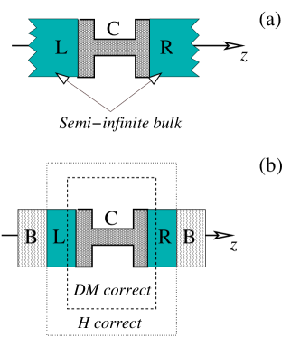
Figure 1: (a) We model the Contact ($C$) region coupled to two semi-infinite Left ($L$) and Right ($R$) electrodes. The direction of transport is denoted by $z$. (b) We only describe a finite section of the infinite system: Inside the $L$ and $R$ parts the Hamiltonian matrix elements have bulk electrode values. The external (Buffer) region, $B$, is not directly relevant for the calculation.

The region of interest is thus separated into three parts, Left ($L$), Contact ($C$) and Right ($R$). The atoms in $L$ ($R$) are assumed to be the parts of the left (right) semi-infinite bulk electrodes with which the atoms in region $C$ interact. The Hamiltonian is assumed to be converged to the bulk values in region $L$ and $R$ along with the density matrix. Thus the Hamiltonian, density and overlap matrices only differ from bulk values in the $C$, $C-L$ and $C-R$ parts. We can test this assumption by including a larger fraction of the electrodes in $C$ (so the $L$ and $R$ regions are positioned further away from the surfaces in Fig. 1).

In order to obtain the transport properties of the system, we only need to describe the finite $L-C-R$ part of the infinite system as illustrated in Fig. 1b. The density matrix which describes the distribution of electrons can be obtained from a series of Green’s function matrices of the infinite system as we will discuss in detail in Section III. In principle the Green’s function matrix involves the inversion of an infinite matrix corresponding to the infinite system with all parts of the electrodes included. We are, however, only interested in the finite $L-C-R$ part of the density matrix and thus of the Green’s function matrix. We can obtain this part by inverting the finite matrix,

𝐕L†𝐇C𝐕R0𝐕R†𝐇R+𝚺R),fragments fragmentsV𝐿†fragmentsH𝐶fragmentsV𝑅0fragmentsV𝑅†fragmentsH𝑅Σ𝑅\left(\begin{tabular}[]{c|c|c}${\bf H}_{L}+{\bf\Sigma}_{L}$&${\bf V}_{L}$&$0$\\ \hline\cr${\bf V}_{L}^{\dagger}$&${\bf H}_{C}$&${\bf V}_{R}$\\ \hline\cr$0$&${\bf V}_{R}^{\dagger}$&${\bf H}_{R}+{\bf\Sigma}_{R}$\\ \end{tabular}\right),

+HLΣLVL0+HLΣLVL0 (1)

where ${\bf H}_{L}$, ${\bf H}_{R}$ and ${\bf H}_{C}$ are the Hamiltonian matrices in the $L$, $R$ and $C$ regions, respectively, and ${\bf V}_{L}$ (${\bf V}_{R}$) is the interaction between the $L$ ($R$) and $C$ regions. The coupling of $L$ and $R$ to the remaining part of the semi-infinite electrodes is fully taken into account by the self-energies, ${\bf\Sigma}_{L}$ and ${\bf\Sigma}_{R}$. We note that to determine ${\bf V}_{L}$, ${\bf V}_{R}$ and ${\bf H}_{C}$, we do not need to know the correct density matrix outside the $L-C-R$ region, as long as this does not influence the electrostatic potential inside the region. This is the case for metallic electrodes, if the $L-C-R$ region is defined sufficiently large so that all the screening takes place inside of it.

The upper and lower part of the Hamiltonian (${\bf H}_{L(R)}+{\bf\Sigma}_{L(R)}$) are determined from two separate calculations for the bulk systems corresponding to the bulk of the left and right electrode systems. These systems have periodic boundary conditions in the $z$ directions, and are solved using Bloch’s theorem. From these calculations we also determine the self-energies by cutting the electrode systems into two semi-infinite pieces using either the ideal constructionWiFeLa82 or the efficient recursion method.LoLoRu84

The remaining parts of the Hamiltonian, ${\bf V}_{L}$, ${\bf V}_{R}$ and ${\bf H}_{C}$, depend on the non-equilibrium electron density and are determined through a selfconsistent procedure. In Section III we will describe how the non-equilibrium density matrix can be calculated given these parts of the Hamiltonian, while in Section IV we show how the effective potential and thereby the Hamiltonian matrix elements are calculated from the density matrix.

III Non-equilibrium Density Matrix

In this section we will first present the relationship between the scattering state approach and the non-equilibrium Green’s function expression for the non-equilibrium electron density corresponding to the situation when the electrodes have different electrochemical potentials. The scattering state approach is quite transparent and has been used for non-equilibrium first principles calculations by McCann and Brown,McBr88 Lang and co-workers,LaYaIm89 ; La95 ; LaAv00 and Tsukada and co-workers.HiTs94 ; HiTs95 ; KoAoTs01 All these calculations have been for the case of model jellium electrodes and it is not straightforward how to extend these methods to the case of electrodes with a realistic atomic structure and a more complicated electronic structure or when localized states are present inside the contact region. The use of the non-equilibrium Green’s functions combined with a localized basis set is able to deal with these points more easily.

Here we will start with the scattering state approach and make the connection to the non-equilibrium Green’s function expressions for the density matrix. Consider the scattering states starting in the left electrode. These are generated from the unperturbed incoming states (labeled by $l$) of the uncoupled, semi-infinite electrode, $\psi^{0}_{l}$, using the retarded Green’s function, $G$, of the coupled system,

$$\psi_{l}(\vec{x})=\psi^{0}_{l}(\vec{x})+\int d\vec{y}\,\,G(\vec{x},\vec{y})\,V_{L}(\vec{y})\,\psi^{0}_{l}(\vec{y})\,.$$ (2)

As in the previous section there is no direct interaction between the electrodes:

$$V(\vec{r}) = V_{L}(\vec{r})+V_{R}(\vec{r})\,.$$ (3)

$$V_{R}(\vec{r})\psi^{0}_{l}(\vec{r}) = V_{L}(\vec{r})\psi^{0}_{r}(\vec{r})=0\,.$$ (4)

Our non-equilibrium situation is described by the following scenario: The states starting deep in the left/right electrode are filled up to the electrochemical potential of the left (right) electrode, $\mu_{L}$ ($\mu_{R}$). We construct the density matrix from the (incoming) scattering states of the left and right electrode:

$$D(\vec{x},\vec{y}) = \sum_{l}\psi_{l}(\vec{x})\psi_{l}^{*}(\vec{y})\,n_{F}({\varepsilon}_{l}-{\mu}_{L})$$ (5)

$$+ \sum_{r}\psi_{r}(\vec{x})\psi_{r}^{*}(\vec{y})\,n_{F}(\varepsilon_{r}-\mu_{R})\,,$$

where index $l$ and $r$ run over all scattering states in the left and right electrode, respectively. Note that this density matrix only describes states in $C$ which couple to the continuum of electrode states – we shall later in Section III.4 return to the states localized in $C$.

III.1 Localized non-orthogonal basis

Here we will rather consider the density matrix defined in terms of coefficients of the scattering states with respect to the given basis (denoted below by Greek subindexes)

$$\psi_{l}(\vec{x})=\sum_{\mu}c_{l\mu}\phi_{\mu}(\vec{x})\,.$$ (6)

Thus (2) and (5) read,

$$c_{l\mu}=c^{0}_{l\mu}+\sum_{\nu}\left({\bf G}(z){\bf V}\right)_{\mu\nu}\,c^{0}_{l\nu}\,\,,\,\,\,z=\varepsilon_{l}+i\delta\,,$$ (7)

$${\bf D}_{\mu\nu} = \sum_{l}c_{l\mu}c_{l\nu}^{*}\,n_{F}(\varepsilon_{l}-\mu_{L})$$ (8)

$$+ \sum_{r}c_{r\mu}c_{r\nu}^{*}\,n_{F}(\varepsilon_{r}-\mu_{R})\,.$$

The basis is in general non-orthogonal but this will not introduce any further complications. As for the Hamiltonian, we assume that the matrix elements of the overlap, ${\bf S}$, are zero between basis functions in $L$ and $R$. The overlap is handled by defining the Green’s function matrix ${\bf G}(z)$ as the inverse of $(z{\bf S-H})$, and including the term $-z{\bf S}$ in the perturbation matrix ${\bf V}$. To see this we use the following equations,

$$\left[\varepsilon_{l}{\bf S}_{0}-{\bf H}_{0}\right]c^{0}_{l} = 0\,,$$ (9)

$$\left[\varepsilon_{l}{\bf S}-{\bf H}\right]c_{l} = 0\,,$$ (10)

$$\left[z{\bf S}-{\bf H}\right]{\bf G}(z) = \openone\,.$$ (11)

With these definitions we see that (7) is fulfilled,

$$\left[\varepsilon_{l}{\bf S}-{\bf H}\right]c_{l}=\left[\varepsilon_{l}{\bf S}-{\bf H}\right]c^{0}_{l}+{\bf V}c^{0}_{l}=0\,,$$ (12)

when

$${\bf V}={\bf H}-{\bf H}_{0}-\varepsilon_{l}({\bf S}-{\bf S}_{0})\,.$$ (13)

The use of a non-orthogonal basis is described further in Refs. WiFeLa82, and EmKi98, .

The density matrix naturally splits into left and right parts. The derivations for left and right are similar, so we will concentrate on left only. It is convenient to introduce the left spectral density matrix, $\rho_{L}$,

$${\bf\rho}^{L}_{\mu\nu}(\varepsilon)=\sum_{l}c_{l\mu}c_{l\nu}^{*}\,\delta(\varepsilon-\varepsilon_{l}),$$ (14)

and likewise a right spectral matrix $\rho_{R}$. The density matrix is then written as,

$${\bf D}_{\mu\nu}=\int_{-\infty}^{\infty}d\varepsilon\,{\bf\rho}^{L}_{\mu\nu}(\varepsilon)n_{F}(\varepsilon-\mu_{L})+{\bf\rho}^{R}_{\mu\nu}(\varepsilon)n_{F}(\varepsilon-\mu_{R})\,.$$ (15)

As always we wish to express ${\bf\rho}^{L}$ in terms of known (unperturbed) quantities, i.e., $c^{0}_{l\mu}$, and for this we use Equation (7). Since we are only interested in the density matrix part corresponding to the scattering region ($L-C-R$), we note that the coefficients $c^{0}_{l\mu}$ for the unperturbed states are zero for basis functions ($\mu$) within this region. Thus

$$c_{l\mu}=\sum_{\nu}\left({\bf G}{\bf V}\right)_{\mu\nu}\,c^{0}_{l\nu}\,\,,$$ (16)

where $\nu$ is inside the bulk of the left electrode. Inserting this in Eq. (14) we get,

$${\bf\rho}^{L}_{\mu\nu}(\varepsilon)=\left({\bf G}(\varepsilon)\frac{1}{\pi}{\mbox{Im}}\left[{\bf V}{\bf g}^{L}(\varepsilon){\bf V}^{\dagger}\right]{\bf G}^{\dagger}(\varepsilon)\right)_{\mu\nu}.$$ (17)

Here we use the unperturbed left retarded Green’s function,

$${\bf g}^{L}_{\mu\nu}(\varepsilon)=\sum_{l}\frac{c^{0}_{l\mu}c_{l\nu}^{0*}}{\varepsilon-\varepsilon_{l}+i\delta}\,\,,$$ (18)

and the relation

$$\left[{\bf g}^{L}(\varepsilon)-({\bf g}^{L}(\varepsilon))^{\dagger}\right]_{\mu\nu}=2\pi i\sum_{l}c^{0}_{l\mu}c_{l\nu}^{0*}\,\delta(\varepsilon-\varepsilon_{l})\,,$$ (19)

and that ${\bf g}={\bf g}^{T}$ due to time-reversal symmetry.

We can identify the retarded self-energy,

$${\bf\Sigma}_{L}(\varepsilon) \equiv \left[{\bf V}{\bf g}^{L}(\varepsilon)\,{\bf V}^{\dagger}\right]\,,$$ (20)

$${\bf\Gamma}_{L}(z) \equiv i\left[{\bf\Sigma}_{L}(\varepsilon)-{\bf\Sigma}_{L}(\varepsilon)^{\dagger}\right]/2\,,$$ (21)

and finally we express ${\bf\rho}^{L}$ as,

$${\bf\rho}^{L}_{\mu\nu}(\varepsilon)=\frac{1}{\pi}\left({\bf G}(\varepsilon){\bf\Gamma}_{L}(\varepsilon){\bf G}^{\dagger}(\varepsilon)\right)_{\mu\nu}\,,$$ (22)

and a similar expression for ${\bf\rho}^{R}$. Note that the ${\bf\Sigma}$, ${\bf\Gamma}$ and ${\bf G}$ matrices in the equations above are all matrices defined only in the scattering region $L-C-R$ which is desirable from a practical point of view. The G matrix is obtained by inverting the matrix in Eq. 1.

The expression derived from the scattering states is the same as one would get from a non-equilibrium Green’s function derivation, see e.g. Refs. HaJa96, , where ${\bf D}$ is expressed via the “lesser” Green’s function,

$${\bf D}=\frac{1}{2\pi i}\int_{-\infty}^{\infty}d\varepsilon\,{\bf G}^{<}(\varepsilon)\,,$$ (23)

which includes the information about the non-equilibrium occupation.

III.2 Complex contour for the equilibrium density matrix

In equilibrium we can combine the left and right parts in Eq. (15),

$${\bf G\Gamma G}^{\dagger} = {i\over 2}{\bf G}\left[{\bf\Sigma}-{\bf\Sigma}^{\dagger}\right]{\bf G}^{\dagger}$$ (24)

$$= -{i\over 2}{\bf G}\left[({\bf G})^{-1}-({\bf G}^{\dagger})^{-1}\right]{\bf G}^{\dagger}$$

$$= -\text{Im}[{\bf G}]$$

where ${\bf\Sigma}$ includes both ${\bf\Sigma}_{L}$ and ${\bf\Sigma}_{R}$, and time-reversal symmetry (${\bf G}^{\dagger}={\bf G}^{*}$) was invoked. With this Eq. (15) reduces to the well-known expression,

$${\bf D} = -\frac{1}{\pi}\int_{-\infty}^{\infty}d\varepsilon\,\,\text{Im}[{\bf G}(\varepsilon+i\delta)]\,n_{F}(\varepsilon-\mu)$$ (25)

$$= -\frac{1}{\pi}\text{Im}\Big{[}\int_{-\infty}^{\infty}d\varepsilon\,{\bf G}(\varepsilon+i\delta)\,n_{F}(\varepsilon-\mu)\Big{]}\,.$$

The invocation of time-reversal symmetry makes ${\bf D}$ a real matrix since ${\bf D}^{*}={\bf D}^{T}={\bf D}$.

At this point it is important to note that we have neglected the infinitesimal $i\delta$ in Eq. (24). This means that the equality in Eq. (24) is actually not true when there are states present in $C$ which do not couple to any of the electrodes, and thus ${\bf\Gamma}_{L}={\bf\Gamma}_{R}=0$ and $\rho_{L}=\rho_{R}=0$ for elements involving strictly localized states. The localized states cannot be reached starting from scattering states and are therefore not included in Eq. (15), while they are present in Eq. (25). We return to this point in Section III.4 below.

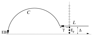
Figure 2: The closed contour: $L$ ($]\infty+i\Delta;EF-\gamma+i\Delta[$), $C$, and $[EB+i\delta;\infty+i\delta]$ enclosing the Fermi poles (black dots).

All poles of the retarded Green’s function ${\bf G}(z)$ are lying on the real axis and the function is analytic otherwise. Instead of doing the integral in Eq. (25) (corresponding to the dotted line in Fig. 2), we consider the contour in the complex plane defined for a given finite temperature shown by the solid line in Fig. 2. Indeed, the closed contour beginning with line segment $L$, followed by the circle segment $C$, and running along the real axis from $(EB+i\delta)$ to $(\infty+i\delta)$, where $EB$ is below the bottom valence band edge, will only enclose the poles of $n_{F}(z)$ located at $z_{\nu}=i(2\nu+1)\pi kT$. According to the residue theorem,

$$\oint dz\,{\bf G}(z)\,n_{F}(z-\mu)=-2\pi i\,kT\sum_{z_{\nu}}{\bf G}(z_{\nu})\,,$$ (26)

where we use that the residues of $n_{F}$ are $-kT$. Thus,

$$\int_{EB}^{\infty}d\varepsilon\,{\bf G}(\varepsilon+i\delta)\,n_{F}(\varepsilon-\mu)$$ (27)

$$=-\int_{C+L}dz\,{\bf G}(z)\,n_{F}(z-\mu)-2\pi i\,kT\sum_{z_{\nu}}{\bf G}(z_{\nu})\,.$$

The contour integral can be computed numerically for a given finite temperature by choosing the number of Fermi poles to enclose. This insures that the complex contour stays away from the real axis (the part close to $EB$ is not important). The Green’s function will behave smoothly sufficiently away from the real axis, and we can do the contour integral by Gaussian quadrature with just a minimum number of points, see Fig. 3. The main variation on $L$ comes from $n_{F}$ and it is advantageous to use $n_{F}$ as a weightfunction in the Gaussian quadrature.gaussfermi

Figure 3: Typical points for Gaussian quadrature on the contour. On $L$ we employ a quadrature with a weight function equal to the Fermi function.

III.3 Numerical procedure for obtaining the non-equilibrium density matrix

In non-equilibrium the density matrix is given by

$${\bf D}_{\mu\nu} = {\bf D}^{L}_{\mu\nu}+\Delta^{R}_{\mu\nu}\,,$$ (28)

$${\bf D}_{\mu\nu}^{L} = -\frac{1}{\pi}\text{Im}\Big{[}\int_{EB}^{\infty}d\varepsilon\,{\bf G}(\varepsilon+i\delta)\,n_{F}(\varepsilon-\mu_{L})\Big{]}\,,$$ (29)

$$\Delta^{R}_{\mu\nu} = \int_{-\infty}^{\infty}d\varepsilon\,{\bf\rho}^{R}_{\mu\nu}(\varepsilon)[n_{F}(\varepsilon-\mu_{R})-n_{F}(\varepsilon-\mu_{L})]\,,$$ (30)

or equivalently

$${\bf D}_{\mu\nu} = {\bf D}^{R}_{\mu\nu}+\Delta^{L}_{\mu\nu}\,,$$ (31)

$${\bf D}_{\mu\nu}^{R} = -\frac{1}{\pi}\text{Im}\Big{[}\int_{EB}^{\infty}d\varepsilon\,{\bf G}(\varepsilon+i\delta)\,n_{F}(\varepsilon-\mu_{R})\Big{]}\,,$$ (32)

$$\Delta^{L}_{\mu,\nu} = \int_{-\infty}^{\infty}d\varepsilon\,{\bf\rho}^{L}_{\mu\nu}(\varepsilon)[n_{F}(\varepsilon-\mu_{L})-n_{F}(\varepsilon-\mu_{R})]\,.$$ (33)

The spectral density matrices, ${\bf\rho}^{L}$ and ${\bf\rho}^{R}$, are not analytical. Thus only the “equilibrium” part of the density matrix, ${\bf D}^{L}$(${\bf D}^{R}$), can be obtained using the complex contour. Furthermore, this is a real quantity due to the time-reversal symmetry, whereas the “non-equilibrium” part, $\Delta^{L}$($\Delta^{R}$) cannot be made real since the scattering states by construction break time-reversal symmetry due to their boundary conditions. The imaginary part of $\Delta^{L}$ ($\Delta^{R}$) is in fact directly related to the local current.Todorov99 However, if we are interested only in the electron density and if we employ a basis-set with real basis functions ($\phi_{\mu}$) we can neglect the imaginary part of ${\bf D}$,

$$n(\vec{r})=\sum_{\mu,\nu}\phi_{\mu}(\vec{r}){\text{Re}}\Big{[}{\bf D}_{\mu\nu}\Big{]}\phi_{\nu}(\vec{r})\,.$$ (34)

To obtain $\Delta^{L}$ ($\Delta^{R}$) the integral must be evaluated for a finite level broadening, $i\delta$, and on a fine grid. Even for small voltages we find that this integral can be problematic, and care must be taken to ensure convergence in the level broadening and number of grid points. Since we have two similar expressions for the density matrix we can get the integration error from

$${\bf e}_{\mu\nu}={\bf D}^{R}_{\mu\nu}+\Delta^{L}_{\mu\nu}-({\bf D}^{L}_{\mu\nu}+\Delta^{R}_{\mu\nu}).$$ (35)

The integration error arises mainly from the real axis integrals, and depending on which entry of the density matrix we are considering either $\Delta^{L}$ or $\Delta^{R}$ can dominate the error. Thus with respect to the numerical implementation the two formulas Eq. (28) and (31) are not equivalent. We will calculate the density matrix as a weighted sum of the two integrals

$${\bf D}_{\mu\nu} = w_{\mu\nu}({\bf D}^{L}_{\mu\nu}+\Delta^{R}_{\mu\nu})+(1-w_{\mu\nu})({\bf D}^{R}_{\mu\nu}+\Delta^{L}_{\mu\nu})$$ (36)

$$w_{\mu\nu} = \frac{(\Delta^{L}_{\mu\nu})^{2}}{(\Delta^{L}_{\mu\nu})^{2}+(\Delta^{R}_{\mu\nu})^{2}}.$$ (37)

The choice of weights can be rationalized by the following argument. Assume that the result of the numerical integration is given by a stochastic variable $\tilde{\Delta}^{L}$ with mean value $\Delta^{L}$ and the standard deviation is proportional to the overall size of the integral, i.e. $Var(\tilde{\Delta}^{L})\propto(\Delta^{L})^{2}$. A numerical calculation with weighted integrals as in Eq. (36) will then be a stochastic variable with the variance

$$Var(\tilde{\bf D})\propto w^{2}(\Delta^{R})^{2}+(1-w)^{2}(\Delta^{L})^{2}.$$ (38)

The value of $w$ which minimize the variance is the weight factor we use in Eq. (37).

III.4 Localized states

As mentioned earlier the signature of a localized state at $\varepsilon_{0}$ in the scattering region is that the matrix elements of ${\bf\Gamma}_{L}(\varepsilon_{0}),{\bf\Gamma}_{R}(\varepsilon_{0})$ are zero for that particular state. Localized states most commonly arise when the atoms in $C$ have energy levels below the bandwidth of the leads. The localized states give rise to a pole at $\varepsilon_{0}$ in the Green’s function. As long as $\varepsilon_{0}<\{\mu_{L},\mu_{R}\}$ the pole will be enclosed in the complex contours and therefore included in the occupied states. If on the other hand the bound state has an energy within the bias window, i.e. $\mu_{L}<\varepsilon_{0}<\mu_{R}$ the bound state will not be included in the real axis integral ($\Delta^{L}$, $\Delta^{R}$) and in the complex contour for ${\bf D}^{L}$, but it will be included in the complex contour for ${\bf D}^{R}$. Such a bound state will only be correctly described by the present formalism if additional information on its filling is supplied. These situations are rare and seldom encountered in practice.

IV The nonequilibrium effective potential

The DFT effective potential consists of three parts: a pseudo potential $V_{ps}$, the exchange correlation potential $V_{xc}$, and the Hartree potential $V_{H}$. For $V_{ps}$ we use norm conserving Troullier-Martins pseudopotentials, determined from standard procedures.TrMa91 For $V_{xc}$ we use the LDA as parametrized in Ref. PeZu81, .

IV.1 The Hartree potential

The Hartree potential is a non-local function of the electron density, and it is determined through the Poisson’s equation (in Hartree atomic units),

$${\nabla}^{2}V_{H}(\vec{r})=-4\pi n(\vec{r})\,.$$ (39)

Specifying the electron density only in the C region of Fig. 1 makes the Hartree potential of this region undetermined up to a linear termnotepoisson ,

$$V_{H}(\vec{r})=\phi(\vec{r})+\vec{a}\cdot\vec{r}+b\,,$$ (40)

where $\phi(\vec{r})$ is a solution to Poisson’s equation in region C and $\vec{a}$ , $b$ are parameters that must be determined from the boundary conditions to the Poisson’s equation. In the directions perpendicular to the transport direction ($x$,$y$) we will use periodic boundary conditions which fix the values of $a_{x}$, $a_{y}$. The remaining two parameters $a_{z}$, $b$ are determined by the value of the electrostatic potential at the $L-C$ and $C-R$ boundaries. The electrostatic potential in the $L$ and $R$ regions could be determined from the separate bulk calculations, and shifted relative to each other by the bias $V$. With these boundary conditions the Hartree potential in the contact is uniquely defined, and could be computed using a real-space technique realspace or an iterative method.HiTs95

However, in the present work, we have solved the Poisson’s equation using a Fast Fourier Transform (FFT) technique. We set up a supercell with the $L-C-R$ region, which can contain some extra layers of buffer bulk atoms and, possibly, vacuum (specially if the two electrodes are not of the same nature, otherwise the $L$ and $R$ are periodically matched in the $z$ direction). We note in passing that this is done so that the potential at the $L-C$ and $C-R$ boundaries reproduces the bulk values, crucial for our method to be consistent. For a given bias, $V$, the $L$ and $R$ electrode electrostatic potentials need to be shifted by $V/2$ and $-V/2$, respectively, and $V_{H}$ will therefore have a discontinuity at the cell boundary. The electrostatic potential of the supercell is now decomposed as:

$$V_{H}(\vec{r})=\widetilde{\phi}(\vec{r})-V(\frac{z}{L_{z}}-0.5).$$ (41)

where $\widetilde{\phi}(r)$ is a periodic solution of the Poisson’s equation in the supercell, and therefore can be obtained using FFT’s.notepoisson2

To test the method we have calculated the induced density and potential on a “capacitor” consisting of two gold (111) surfaces separated by a 12 bohr wide tunnelgap and with a voltage drop of 2 Volt. We have calculated the charge density and the potential in this system in two different ways. First, we apply the present formulation (implemented in TranSiesta), where the system consists of two semi-infinite gold electrodes, and the Hartree potential is computed as described above. Then, we calculate a similar system, but with a slab geometry, computing the Hartree potential with Siesta, adding the external potential as a ramp with a discontinuity in the vacuum region. Fig. 4 shows the comparison of the results for the average induced density and potential along the $z$ axis. Since the tunnel gap is so wide that there is no current running, the two methods should give very similar results, as we indeed can observe in the Figure. We can also observe that the potential ramp is very effectively screened inside the material, so that the potential is essentially equal to the bulk one, except for the surface layer. This justifies our approach for the partition of the system, the solution of the Poisson’s equation, and the use of the bulk Hamiltonian matrix elements fo the $L$ and $R$ regions (see below).

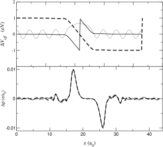
Figure 4: (a) The induced external potential for slab calculation (full line), and in the TranSiesta calculation (dashed line). In the slab calculation the jump in external potential is in the middle of the vacuum region. The total potential (arbitrary units) is shown for reference (dotted line). (b) Induced density. Potential and density is averaged in the surface plane. The density corresponds to one surface unit cell.

IV.2 The Hamiltonian matrix elements

Having determined the effective potential we calculate the Hamiltonian matrix elements as in standard Siesta calculations. However, since we only require the density and the electrostatic potential to be correct at the $L-C$ and $C-R$ boundaries, the ${\bf H}_{L}$ and ${\bf H}_{R}$ parts of the Hamiltonian (see Eq. (1)) will not be correct. We therefore substitute ${\bf H}_{L}$ and ${\bf H}_{R}$ with the Hamiltonian obtained from the calculation of the separate bulk electrode systems. Here it is important to note that the effective potential within the bulk electrode calculations usually are shifted rigidly relative to the effective potential in the $L$ and $R$ regions, due to the choice of the parameter $b$ in Eq. (40). However, the bulk electrode Hamiltonians ${\bf H}_{L}$ and ${\bf H}_{R}$ can easily be shifted, using the fact that the electrode Fermi level should be similar to the Fermi level of the initial Siesta calculation for the BLCRB supercell.

The discontinuity of the Hartree potential at the cell boundary has no consequence in the calculation: the Hamiltonian matrix elements inside the $L-C-R$ region are unaffected because of the finite range of the atomic orbitals, and the Hamiltonian matrix elements outside the $L-C-R$ region which do feel the discontinuity are replaced by bulk values (shifted according to the bias).

V Conductance formulas

Using the non-equilibrium Green’s function formalism (see e.g. Refs. HaJa96, ; Datta, ; BrKoTs99, and references therein) the current, $I$, through the contact can be derived

$$I(V)=G_{0} \int_{-\infty}^{\infty}d\epsilon\,\left(n_{F}(\epsilon-\mu_{L})-n_{F}(\epsilon-\mu_{R})\right)$$ (42)

$${\text{Tr}}\left[{\bf\Gamma}_{L}(\epsilon){\bf G}^{\dagger}(\epsilon){\bf\Gamma}_{R}(\epsilon){\bf G}(\epsilon)\right]\,,$$

where $G_{0}=2e^{2}/h$. We note that this expression is not general but is valid for mean-field theory like DFT.MeWi92 An equivalent formula has been derived by Todorov et al. ToBrSu93 (the equivalence can be derived using Eq. (21) and the cyclic invariance of the trace in Eq. 42).

With the identification of the (left-to-right) transmission amplitude matrix ${\bf t}$,CuYeMR98

$${\bf t}(\epsilon)=\left({\bf\Gamma}_{R}(\epsilon)\right)^{1/2}{\bf G}(\epsilon)\left({\bf\Gamma}_{L}(\epsilon)\right)^{1/2}\,,$$ (43)

(42) is seen to be equivalent to the Landauer-Büttiker formulaBuImLa85 for the conductance, $G=I/V$,

$$G(V) = \frac{G_{0}}{V}\int_{-\infty}^{\infty}d\varepsilon\,[n_{F}(\varepsilon-\mu_{L})-n_{F}(\varepsilon-\mu_{R})]$$ (44)

$${\text{Tr}}\left[{\bf t}^{\dagger}{\bf t}\right](\varepsilon)\,,$$

The eigenchannels are defined in terms of the (left-to-right) transmission matrix ${\bf t}$,Buttike88a ; MaLa92

$${\bf t}\,=\,{\bf U}_{R}\,\mbox{diag}\{|\tau_{n}|\}\,{\bf U}_{L}^{\dagger}\,,$$ (45)

and split the total transmission into individual channel contributions,

$$T_{\text{Tot}}=\sum_{n}\,|\tau_{n}|^{2}\,.$$ (46)

The collection of the individual channel transmissions $\{|\tau_{n}|^{2}\}$ gives a more detailed description of the conductance and is useful for the interpretation of the results.BrSoJa97 ; CuYeMR98 ; BrKoTs99

VI Applications

VI.1 Carbon wires/Aluminum (100) electrodes

Short monoatomic carbon wires coupled to metallic electrodes have recently been studied by Lang and AvourisLaAv98 ; LaAv00 and Larade et al. LaTaMeGu01 . Lang and Avouris used the Jellium approximation for the electrodes, while Larade et al. used Al electrodes with a finite cross section oriented along the (100) direction. In this section, we will compare the TranSiesta method with these other first principles electron transport methods by studying the transmission through a 7-atom carbon chain coupled to Al(100) electrodes with finite cross sections as well as to the full Al(100) surface.

We consider two systems, denoted A and B, shown in Fig. 5a,b. System A consists of a 7-atom carbon chain coupled to two electrodes of finite cross section oriented along the Al(100) direction (see Fig. 5a). The electrode unit cell consists of 9 Al atoms repeated to $z=\pm\infty$. The ends of the carbon chain are positioned in the Al(100) hollow site and the distance between the ends of the carbon chain and the first plane of Al atoms is fixed to be $d=1.0$ Å. In system B the carbon chain is coupled to two Al(100)-($2\sqrt{2}\times 2\sqrt{2}$) surfaces with an Al-C coupling similar to system A. In this case the electrode unit cell contains 2 layers each with 8 atoms. For both systems the contact region ($C$) includes 3 layers of atoms in the left electrode and 4 layers of the right electrode. We use single-$\zeta$ basis sets for both C and Al to be able to compare with the results from McDCAL, which were obtained with that basis.LaTaMeGu01

The conductance of system A is dominated by the alignment of the LUMO state of the isolated chain to the Fermi level of the electrodes through charge transfer.LaTaMeGu01 The coupling of the LUMO, charge transfer, and total conductance can be varied continuously by adjusting the electrode-chain separation.LaTaMeGu01 For our value of the electrode-chain separation we get a charge transfer of 1.43 and 1.28 $e$ to the carbon wire in systems A and B, respectively. This is slightly larger than the values obtained by Lang and AvourisLaAv00 for Jellium electrodes, but in good agreement with results from McDCAL.LaTaMeGu01

To facilitate a more direct comparison between the methods we show in Fig. 6 the transmission coefficient of system A calculated both within TranSiesta (solid) and McDCAL (dotted). For both methods, we have used identical basis sets and pseudopotentials. However, several technical details in the implementations differ and may lead to small differences in the transmission spectra. The main implementation differences between the two methods are related to the calculation of Hamiltonian parameters for the electrode region, the solution of the Poisson’s equation, and the complex contours used to obtain the electron charge.trans-mcdcal Thus, there are many technical differences in the two methods, and we therefore find the close agreement in Fig. 6 very satisfactory.

In Fig. 7 we show the corresponding transmission coefficients for system B. It can be seen that the transmission coefficient for zero bias at $\varepsilon=\mu$ is close to 1 for both systems, thus they have similar conductance. However, the details in the transmission spectra differs much from system A. In order to get some insight into the origin of the different features we have projected the selfconsistent Hamiltonian onto the carbon orbitals, and diagonalised this subspace Hamiltonian to find the position of the carbon eigenstates in the presence of the Al electrodes. Within the energy window shown in Fig. 6 and 7 we find 4 doubly degenerate $\pi$-states (3$\pi$, 4$\pi$, 5$\pi$, 6$\pi$). The positions of the eigenstates are indicated above the transmission curves. Each doubly degenerate state can contribute to the transmission with 2 at most. Generally, the position of the carbon $\pi$ states give rise to a slow variation in the transmission coefficient, and the fast variation is related to the coupling between different scattering states in the electrodes and the carbon $\pi$-states. For instance in system A, there are two energy intervals [-1.9,-1.7] and [0.7,1.4], where the transmission coefficient is zero, and the scattering states in these energy intervals are therefore not coupling to the carbon wire. Note how these zero transmission intervals are doubled at finite bias, since the scattering states of the left and right electrode are now displaced.

The energy dependence of the transmission coefficient is quite different in system B compared to system A. This is mainly due to the differences in the electronic structure of the surface compared to the finite sized electrode. However, the electronic states of the carbon wires are also slightly different. We find that the $\pi$-states lie $~{}0.2$ eV higher in energy in system B relative to system A. As mentioned previously, the charge transfer to the carbon chain is different in the two systems. The origin of this is related to a larger work function ($\sim 1$eV) of the surface relative to the lead. We note that the calculated work function of the surface is 0.76 eV higher than the experimental workfunction of Al (4.4 eV),CRC94 which may be due to the use of a single-$\zeta$ basis set and the approximate exchange-correlation description.SkRo92

In Fig. 5d, we show the changes in the effective potential when a 1 V bias is applied. We find that the potential does not drop continuously across the wire. In system A, the main potential drop is at the interface between the carbon wire and the right electrode, while in system B the potential drop takes place at the interface to the left electrode. This should be compared to the Jellium results, where there is a more continuous voltage drop through the system.LaAv00 We do not yet understand the details of the origin of these voltage drops. However, it seems that the voltage drop is very sensitive to the electronic structure of the electrodes. Thus, we find it is qualitatively and quantitatively important to have a good description of the electronic structure of the electrodes.

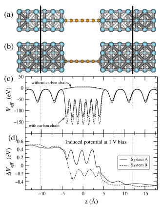
Figure 5: (a) The 7-atom carbon chain with finite cross section Al(100) electrodes(system A). (b) The carbon chain with Al(100)-($2\sqrt{2}\times 2\sqrt{2}$) electrodes(system B). (c) The effective potential of system A(dashed) and system B(solid), together with the effective potential of the corresponding bare electrode systems. (d) The selfconsistent effective potential for an external bias of 1 V (the zero bias effective potential has been subtracted).

Figure 6: (a) Zero bias transmission coefficient, $T(E,0V)$, for the 7-atom carbon chain with finite cross section Al(100) electrodes (system A). (b) Transmission coefficient at 1 V, $T(E,1V)$. Solid lines show results obtained with TranSiesta, and dotted lines results obtained with McDCAL. The vertical dashed lines indicated the window between $\mu_{L}$ and $\mu_{R}$. The position of the eigenstates of the carbon wire subsystem are also indicated at the top axis.

Figure 7: Transmission coefficients, $T(E,0V)$ and $T(E,1V)$ for the 7-atom carbon chain with Al(100)-($2\sqrt{2}\times 2\sqrt{2}$) electrodes(system B). The position of the eigenstates of the carbon wire subsystem are also indicated at the top axis.

VI.2 Gold wires/Gold (111) electrodes

The conductance of single atom gold wires is a benchmark in atomic scale conduction. Since the first experimentsAgRoVi93 ; PaMeGo93 ; OlLaSt94 numerous detailed studies of their conductance have been carried out through the 1990s until now (see e.g. Ref. Ruiten00, for a review). More recently the non-linear conductanceYaSa97 ; CoCoZh99 ; HaNiBr00 ; YuEnSa01 has been investigated and the atomic structureOhKoTa98 ; RoFuUg00 ; RoUg01 of these systems has been elucidated. Experiments show that chains containing more than 5 gold atomsYaBoBr98 can be pulled and that these can remain stable for an extended period of time at low temperature. A large number of experiments employing different techniques and under a variety of conditions (ambient pressure and UHV, room and liquid He temperature) all show that the conductance at low bias is very close to 1 $G_{0}$ and several experiments point to the fact that this is due to a single conductance eigenchannel.ScAgCu98 ; BrRu99 ; LuDeEs99

Several theoretical investigations have addressed the stability and morphology ToToCoErKoToSo99 ; SaArJu99 ; OkTa99 ; HaBaLa99 ; MaSp00 ; HaBaSc00 and the conductance OkTa99 ; HaBaLa99 ; HaBaSc00 of atomic gold chains and contacts using DFT. However, for the evaluation of the conductance, these studies have neglected the presence of valence $d$-electrons and the scattering due to the non-local pseudopotential. This approximation is not justified a priori: for example, it is clear that the bands due to $d$-states are very close to the Fermi level in infinite linear chains of gold and this indicates that these could play a role, especially for a finite bias.BrKoTs99

VI.2.1 Model

In this section we consider gold wires connected between the (111) planes of two semi-infinite gold electrodes. In order to keep the computational effort to a minimum we will limit our model of the electrode system to a small unit cell ($3\times 3$) and use only the $\Gamma$-point in the transverse (surface) directions. We have used a single-$\zeta$ plus polarization basis set of 9 orbitals corresponding to the $5d$ and $6(s,p)$ states of the free atom. In one calculation (the wire labelled (c) in Fig. 9) we used double-$\zeta$ representation of the $6s$ state as a check and found no significant change in the results. The range of interaction between orbitals is limited by the radii of the atomic orbitals to 5.8 Å, corresponding to the 4th nearest neighbor in the bulk gold crystal or a range of three consecutive layers in the [111] direction. We have checked that the bandstructure of bulk gold with this basis set is in good agreement with that obtained with more accurate basis sets for the occupied and lowest unoccupied bands.

We have considered two different configurations of our calculation cell, shown in Fig. 8. In most calculations we include two surface layers in the contact region ($C$) where the electron density matrix is free to relax and we have checked that these results do not change significantly when three surface layers are included on both electrodes. We obtain the initial guess for a density matrix at zero bias voltage from an initial Siesta calculation with normal periodic boundary conditions in the transport ($z$) direction.siestaprecalc In order to make this density matrix as close to the TranSiesta density matrix we can include extra layers in the interface between the $L$ and $R$ regions (black atoms in Fig. 8) to simulate bulk. In the case of two different materials for $L$ and $R$ electrodes many layers may be needed, but in this case we use just one layer. We use the zero bias TranSiesta density matrix as a starting point for TranSiesta runs with finite bias.

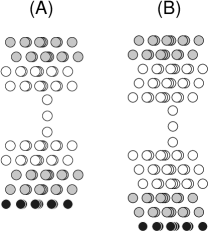
Figure 8: Models used for the gold wires calculations. The white atoms correspond to contact region $C$ while the grey atoms correspond to the $L$ and $R$ regions in Fig. 1. The black atoms are only included in the initial Siesta calculation and can be added in order to yield a better initial density matrix for the subsequent TranSiesta run. We have used 2(A) and 3(B) surface layers in the contact region.

VI.2.2 Bent wires

In a previous study by Sánchez-Portal and co-workers,SaArJu99 a zig-zag arrangement of the atoms was found to be energetically preferred over a linear structure in the case of infinite atomic gold chains, free standing clusters, and short wires suspended between two pyramidal tips. In general the structure of the wires will be determined by the fixed distance between the electrodes and the wires will therefore most probably be somewhat compressed or stretched.

Here we have considered wires with a length of three atoms and situated between the (111) electrodes with different spacing. Initially the wire atoms are relaxed at zero voltage bias (until any force is smaller than 0.02 eV/Å) and for fixed electrode atoms. The four relaxed wires for different electrode spacings are shown in Fig. 9(a)-(d). The values for bondlength and bondangle of the first wire (a), $r=2.57$ Å, $\alpha=135^{\circ}$, are close to the values found in Ref. SaArJu99, for the infinite periodic wires at the minimum of energy with respect to unit-cell length ($r=2.55$  Å, $\alpha=131^{\circ}$).

Figure 9: We have considered the distances 9.0 (a), 9.3 (b), 9.6 (c) and 9.9 (d) Å between the two (111) surfaces. All wires have been relaxed while the surface atoms are kept fixed. Distances are shown in Å.

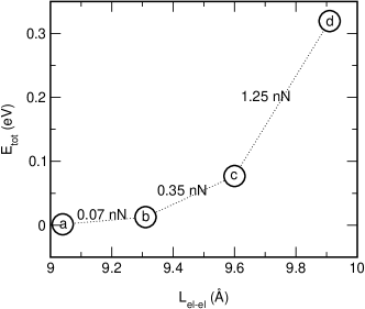
Figure 10: The change in total energy of the relaxed wires during the elongation shown in Fig. 9 as calculated in a Siesta run. The force determined from the slopes of the line segments is shown also.

In Fig. 10 we show the total energy and corresponding force as evaluated in a standard Siesta calculation for the wires as a function of electrode spacing. The force just before the stretched wire breaks has been measuredRuAgVi96 ; RuBaAg01 and is found to be 1.5$\pm$0.3 nN independent of chain length. The total transmission resolved in energy is shown in Fig. 11 for zero bias. The conductance in units of $G_{0}$ is given by $T_{\text{Tot}}(E_{F})$ which is $0.91$, $1.00$, $0.95$, and $0.94$ for the (a), (b), (c), and (d) structures of Fig. 9, respectively. It is striking that the measured conductance in general stays quite constant as the wire is being stretched. Small dips below 1 $G_{0}$ can be seen, which might be due to additional atoms being introduced into the wire from the electrodes during the pull.RuBaAg01 It is interesting to note that the value for (a) is quite close to the conductance dip observed in Ref. RuBaAg01, and we speculate that this might correspond to the addition of an extra atom in the chain which will then attain a zig-zag structure which is subsequently stretched out to a linear configuration.

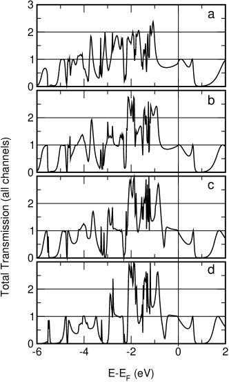
Figure 11: The total transmission of the wires shown in Fig. 9 vs. electron energy.

It can be seen from the corresponding eigenchannel decomposition in Fig. 12 that the conductance is due to a single, highly transmitting channel, in agreement with the experiments mentioned earlier and previous calculations.BrSoJa97 ; CuYeMR98 ; BrKoTs99 ; HaBaSc00 This channel is composed of the $l_{z}=0$ orbitals.BrKoTs99 About $0.5-1.0$ eV below the Fermi energy transmission through additional channels is seen. These are mainly derived from the $l_{z}=1$ orbitals and are degenerate for the wires without a bend, due to the rotational symmetry.

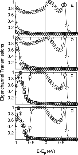
Figure 12: Eigenchannel transmissions of the wires in Fig. 9. Only three channels give significant contribution within the energy range shown.

We have done a calculation for a 5 atom long wire. The relaxed structure is shown in Fig. 13. We note that while the bondlengths are the same within the wire, there is a different bondangle ($143^{\circ}$ in the middle, $150^{\circ}$ at the electrodes). We find that the transmission at zero bias is even closer to unity compared with the 3 atom case and find a conductance of 0.99 $G_{0}$ despite its zig-zag structure.

Figure 13: Relaxed structure of a 5 atom long chain. Distances are shown in Å.

Figure 14: The total transmission of all channels and eigenchannel transmissions of the 5 atom long chain shown in Fig. 13.

VI.2.3 Finite bias results

Most experimental studies of atomic wires have been done in the low voltage regime ($V<0.25$ V). Important questions about the nonlinear conductance, stability against electromigration and heating effects arises in the high voltage regime. It has been found that the single atom gold wires can sustain very large current densities, with an intensity of up to 80$\mu$A corresponding to 1 V bias.YaBoBr98 Sakai and co-workersYaSa97 ; ItYuKu99 ; YuEnSa01 have measured the conductance distributions (histograms) of commercial gold relays at room temperature and at 4K and found that the prominent 1 $G_{0}$ peak height decreases for high biases $V>1.5$ V and disappears around 2 V. It is also observed that there is no shift in the 1 $G_{0}$ peak position which indicates that the nonlinear conductance is small. In agreement with this Hansen et al.HaNiBr00 reported linear current-voltage ($I$-$V$) curves in STM-UHV experiments and suggested that nonlinearities are related with presence of contaminants. On the theoretical side $s,p,d$-tight-binding calculationsBrKoTs99 ; HaNiBr00 has been performed for voltages up to 2.0 V for atomic gold contacts between (100),(111) and (110) electrodes. Todorov et al.ToHoSu00 ; ToHoSu01 has addressed the forces and stability of single atom gold wires within a single orbital model combined with the fixed atomic charge condition.

Here we study the influence of such high currents and fields on one of the wire structures ((c) in Fig. 9). We have performed the calculations for voltages from 0.25 V to 2.0 V in steps of 0.25 V. In Fig. 15 we show the eigenchannel transmissions for finite applied bias. For a bias of 0.5 V we see a behavior similar to the 0 V situation except for the disappearance of the resonance structure about 0.7 eV above $E_{F}$ in Fig. 12(c). For 0.5 V bias the degenerate peak 0.75 eV below $E_{F}$ which is derived from the $l_{z}=1$ orbitals is still intact whereas this feature diminishes gradually for higher bias. Thus mainly a single channel contributes for finite bias up to 2 V. It is clear from Fig. 15 that the transmissions for zero volts cannot be used to calculate the conductance in the high voltage regime and underlines the need for a full self-consistent calculation.

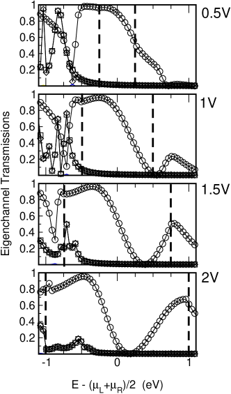
Figure 15: The eigenchannel transmissions for bias voltages of 0.5 V, 1 V, 1.5 V, and 2 V for the wire shown in Fig. 9. The conductance is determined from the average total transmission from $\mu_{L}$ to $\mu_{R}$. The voltage window is shown with thick dashed lines.

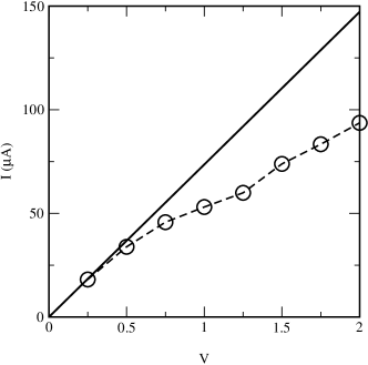
Figure 16: The current-voltage ($I$-$V$) curve for the wire shown in Fig. 9.

The calculated $I$-$V$curve is shown in Fig. 16. We observe a significant decrease in the conductance ($I/V$) for high voltages. This is in agreement with tight-binding resultsBrKoTs99 where a 30% decrease was observed for a bias of 2 V. For wires attached to (100) and (110) electrodesBrKoTs99 ; HaNiBr00 a quite linear $I$-$V$was reported for the same voltage range.

In Fig. 17 and Fig. 18 we plot the voltage drop - i.e. the change in total potential between the cases of zero and finite bias, for the case of 1 V and 2 V, respectively. We observe that the potential drop has a tendency to concentrate in between the two first atoms in the wire in the direction of the current. A qualitatively similar behavior was seen in the tight-binding results for both (100) and (111) electrodesBrKoTs99 and it was suggested to be due to the details of the electronic structure with a high density of states just below the Fermi energy derived from the $d$ orbitals (and their hybridization with $s$ orbitals). The arguments were based on the atomic charge neutrality assumption. In the present calculations, this assumption is not made, although the selfconsistency and the screening in the metallic wire will drive the electronic distribution close to charge neutrality. This would not occur in the case of a non-metallic contact.PaPeLoVe01 ; TaGuWa01a

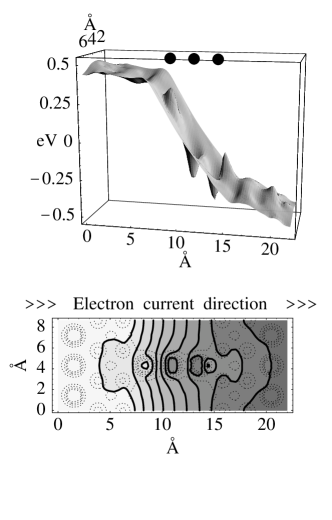
Figure 17: The voltage drop for applied bias of 1 V in a plane going through the wire atoms. In the surface plot the wire atom positions are shown as black spheres. In the contour plot below the solid contours (separated by 0.1 eV) show the voltage drop. The dashed contours are shown to indicate the atomic positions.

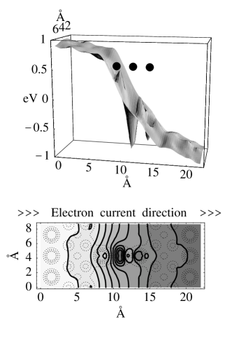
Figure 18: Same as in Fig. 17 for a bias of 2 V (contours separated by 0.2 eV).

The number of valence electrons on the gold atoms is close to 11. There is some excess charge on the wire atoms and first surface layers (mainly taken from the second surface layers). The behavior of the charge with voltage is shown in Fig. 19. The minimum in voltage drop around the middle atom for high bias (see Fig. 18) is associated with a decrease in its excess charge for high bias. The decrease is found mainly in the $s$ and $d_{zz}$ orbitals of the middle atom.

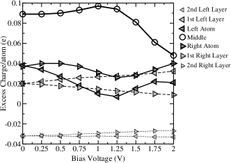
Figure 19: The (Mulliken) change in excess charge (in units of the electron charge) on the wire atoms and average excess charge on the surface atoms in the first and second left and right electrode layers. For high bias the 2nd right electrode layer takes up some of the excess charge.

VI.2.4 Forces for finite bias

We end this section by showing the forces acting on the three atoms in the wire for finite bias in Fig. 20. We evaluate the forces for non-equilibrium in the same manner as for equilibrium Siesta calculationsOrArSo96 by just using the nonequilibrium density matrix and Hamiltonian matrix instead of the equilibrium quantities.ToHoSu00 We find that for voltages above 1.5 V that the first bond in the chain wants to be elongated while the second bond wants to compress. Thus the first bond correspond to a “weak spot” as discussed by Todorov et al.ToHoSu00 ; ToHoSu01 We note that the size of the bias induced forces acting between the two first wire atoms at 2 V is close to the force required to break single atom contactsRuBaAg01 (1.5$\pm$0.3 nN) and the result therefore suggests that the contact cannot sustain a voltage of this magnitude, in agreement with the relay experiments.YuEnSa01 A more detailed calculation including the relaxation of the atomic coordinates for finite voltage bias is needed in order to draw more firm conclusions about the role played by the nonequilibrium forces on the mechanical stability of the atomic gold contacts. We will not go further into the analysis of the electronic structure and forces for finite bias in the gold wire systems at this point, since our aim here is simply to present the method and show some of its capabilities. A full report of our calculations will be published elsewhere.

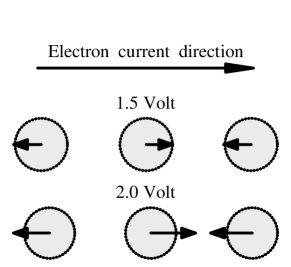
Figure 20: The forces acting on the wire atoms when the bias is applied (the radius of the circles correspond to 0.5 nN). The tensile force in the bond between the two first atoms is about 1 nN for 1 V and 1.5 nN for 2 V.

VI.3 Conductance in nanotubes

Finally, we have applied our approach to the calculation of conductance of nanotubes in the presence of point defects. In particular the Stone-Wales (SW) defectstonewalles (i.e., a pentagon-heptagon double pair) and a monovacancy in a $(10,10)$ nanotube. The atomic geometries of these structures are obtained from a Siesta calculation with a 280-atom supercell (7 bulk unit cells), where the ionic degrees of freedom are relaxed until any component of the forces is smaller than 0.02 eV/Å. We use a single-$\zeta$ basis set, although some tests were made with a double-$\zeta$ basis, producing very similar results. The one dimensional Brillouin zone is sampled with five k-points. The forces do not present any significant variation if the the relaxed configurations are embedded into a 440-atom cell, where the actual transport calculations are performed.

In a perfect nanotube two channels, of character $\pi$ and $\pi^{*}$, contribute each with a quantum of conductance, $G_{0}$. In Fig. 21 we present our results for zero bias for the SW defect. Recent ab initio studies ChIh99 ; ChIhLoCo00 are well reproduced, with two well defined reflections induced by defect states. The two dips in the conductance correspond to the closure of either the $\pi^{*}$ (below the Fermi level) or the $\pi$ channel.

For the ideal vacancy the two antibonding states associated with broken $\sigma$ bonds lie close to the Fermi level. The coupling between these states and the $\pi$ bands, although small, suffices to open a small gap in the bulklike $\pi-\pi^{*}$ bands. The vacancy-induced states appear within this gap. Otherwise, the three two-coordinated atoms have a large penalty in energy and undergo a large reconstruction towards a split vacancy configuration with two pentagons, $\sim 2$ eV lower in energy. Two configurations are possible, depending on the orientation of the pentagon pair, depicted in Fig. 22. We have found that there is a further $0.4$ eV gain in energy by reorienting the pentagon-pentagon $60^{o}$ off the tube axis (Fig. 22b) resulting in a formation energy of $E_{f}=6.75$ eV.ef-def The bonding of the tetracoordinated atom is not planar but paired with angles of $\sim 158^{0}$. Some of these structures were discussed in previous tight-binding calculations.AjRaCh98 This is at variance with the results of Refs. ChIh99, ; ChIhLoCo00, , possibly due to their use of too small a supercell which does not accommodate the long range elastic relaxations induced by these defects.

The conductance of these defects, calculated at zero bias (Fig. 23), does not present any features close to the Fermi level. This is in contrast to the ideal vacancy, where reflection related to the states mentioned above are present. Two dips appear, at possitions similar to those of the SW deffect. An eigenchannel analysisBrSoJa97 of the transmission coefficients gives the symmetry of the states corresponding to these dips. The metastable configuration is close to having a mirror plane, containing the tube axis, except for the small pairing mode mentioned before. The mixing of the $\pi$ and $\pi^{*}$ bands is rather small. The lower and upper dips come from the reflection of the almost pure $\pi^{*}$ and $\pi$ eigenchannels, respectively. This behavior is qualitatively similar to the SW defect. On the other hand, for the rotated pentagon pair there is no mirror plane and the reflected wave does not have a well defined character.

Figure 21: Transmission coefficient of pentagon-heptagon double pair vs. energy measured with respect to the Fermi level. The dotted line shows the transmission of a perfect nanotube.

(a)

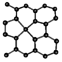
(b)

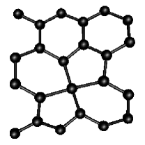
Figure 22: Atomic configurations for the vacancy defect in a (10,10) nanotube: (a) metastable and (b) ground state.

Figure 23: Similar to Fig. 21 but now for the vacancy: ground (continuous line) and metastable (dashed line) configurations.

VII Conclusion

We have described a method and its implementation(TranSiesta) for calculating the electronic structure, electronic transport, and forces acting on the atoms at finite voltage bias in atomic scale systems. The method deals with the finite voltage in a fully self-consistent manner, and treats both the semi-infinite electrodes and the contact region with the same atomic detail.

We have considered carbon wires connected to aluminum electrodes where we find good agreement with results published earlier with another method (McDCAL)LaTaMeGu01 for electrodes with finite cross section. We find that the voltage drop through the wire system depends on the detailed structure of the electrodes (i.e. periodic boundary conditions vs. cross section).

The conductance of three and five atom long gold wires with a bend angle has been calculated. We find that the conductance is close to one quantum unit of conductance and that this result is quite stable against the bending of the wire. These results are in good agreement with experimental findings. For finite bias we find a non-linear conductance in agreement with previous semi-empirical calculations for (111) electrodes.BrKoTs99 We find that the forces at finite bias are close to the experimental force needed to break the gold wiresRuBaAg01 for a bias of 1.5 to 2.0 V.

Finally we have studied the transport through a (10,10) nanotube with a the Stone-Wales defect or with a monovacancy (a calculation involving 440 atoms). We have found good agreement with recent ab initio studies of these systems.ChIh99 ; ChIhLoCo00

- (1) P. Fulde, Electron Correlations in Molecules and Solids (Springer, Berlin, 1995).
- (2) P. Hohenberg and W. Kohn, Phys. Rev. 136, B864 (1964).
- (3) W. Kohn and L. J. Sham, Phys. Rev. 140, A1133 (1965).
- (4) W. Kohn, A. D. Becke, and R. G. Parr, J. Phys. Chem. 100, 12974 (1996).
- (5) R. G. Parr and W. Yang, Density-Functional Theory of Atoms and Molecules (Oxford University Press, New York, 1989).
- (6) Time-dependent DFT and XC functionals depending on the current density [G. Vignale and W. Kohn, Phys. Rev. Lett. 77, 2037 (1996)] would be a next step towards a more rigourous foundation of the theory.
- (7) S. Kurth, J. P. Perdew, and P. Blaha, Int. J. Quantum Chem. 75, 889 (1999).
- (8) H. Ness, S. A. Shevlin, and A. J. Fisher, Phys. Rev. B 63, 125422 (2001).
- (9) P. L. Pernas, A. Martin-Rodero, and F. Flores, Phys. Rev. B 41, R8553 (1990).
- (10) W. Tian and S. Datta, Phys. Rev. B 49, 5097 (1994).
- (11) L. Chico, M.P.L. Sancho, and M.C. Mu noz, Phys. Rev. Lett. 81, 1278 (1998).
- (12) A.L.V. de Parga, O. S. Hernan, R. Miranda, A. Levy Yeyati, A. Martin-Rodero, and F. Flores, Phys. Rev. Lett. 80, 357 (1998).
- (13) E. G. Emberly and G. Kirczenow, Phys. Rev. B 60, 6028 (1999).
- (14) M. Brandbyge, N. Kobayashi, and M. Tsukada, Phys. Rev. B 60, 17064 (1999).
- (15) H. Mehrez, J. Taylor, H. Guo, J. Wang, and C. Roland, Phys. Rev. Lett. 84, 2682 (2000).
- (16) P. Sautet and C. Joachim, Surf. Sci. 271, 387 (1992).
- (17) L. E. Hall, J. R. Reimers, N. S. Hush, and K. Silverbrook, J. Chem. Phys. 112, 1510 (2000).
- (18) V. Mujica, A. E. Roitberg, and M. A. Ratner, J. Phys. Chem. 112, 6834 (2000).
- (19) F. Biscarini, C. Bustamante, and V. M. Kenkre, Phys. Rev. B 51, 11089 (1995).
- (20) H. Ness and A. Fisher, Phys. Rev. Lett. 83, 452 (1999).
- (21) M. B. Nardelli, Phys. Rev. B 60, 7828 (1999).
- (22) M. B. Nardelli and J. Bernholc, Phys. Rev. B 60, R16338 (1999).
- (23) N. D. Lang, Phys. Rev. B 52, 5335 (1995).
- (24) K. Hirose and M. Tsukada, Phys. Rev. B 51, 5278 (1995).
- (25) S. N. Yaliraki, A. E. Roitberg, C. Gonzalez, V. Mujica, and M. A. Ratner, J. Phys. Chem. 111, 6997 (1999).
- (26) P. A. Derosa and J. M. Seminario, J. Phys. Chem. B 105, 471 (2001).
- (27) J. J. Palacios, A. J. Pérez-Jiménez, E. Louis, and J. A. Vergés, Phys. Rev. B 64, 115411 (2001).
- (28) C. C. Wan, J.-L. Mozos, G. Taraschi, J. Wang, and H. Guo, Appl. Phys. Lett. 71, 419 (1997).
- (29) H. J. Choi and J. Ihm, Phys. Rev. B 59, 2267 (1999).
- (30) S. Corbel, J. Cerda, and P. Sautet, Phys. Rev. B 60, 1989 (1999).
- (31) J. Taylor, H. Guo, and J. Wang, Phys. Rev. B 63, 121104R (2001).
- (32) J. Taylor, H. Guo, and J. Wang, Phys. Rev. B 63, 245407 (2001).
- (33) D. Sanchez-Portal, P. Ordejon, E. Artacho, and J. M. Soler, Int. Journ. of Quantum Chem. 65, 453 (1999).
- (34) N. Troullier and J. L. Martins, Phys. Rev. B 43, 1993 (1991).
- (35) O. F. Sankey and D. J. Niklewski, Phys. Rev. B 40, 3979 (1989).
- (36) E. Artacho, D. Sánchez-Portal, P. Ordejón, A. García, and J. M. Soler, phys. status solidi (b) 215, 809 (1999).
- (37) P. Ordejon, phys. status solidi (b) 217, 335 (2000).
- (38) P. Ordejón, E. Artacho, R. Cachau, J. Gale, A. García, J. Junquera, J. Kohanoff, M. Machado, D. Sánchez-Portal, J. M. Soler, and R. Weht, in Advances in Materials Theory and Modeling – Bridging over Multiple-Length and Time Scales, edited by V. Bulatov, F. Cleri, L. Colombo, L. Lewis, and N. Mousseau, MRS Symposia Proceedings Vol. 677, (Materials Research Society, San Francisco, 2001), p. AA9.6
- (39) H. Haug and A.-P. Jauho, Quantum kinetics in transport and optics of semiconductors (Springer-Verlag, Berlin, 1996).
- (40) S. Datta, in Electronic Transport in Mesoscopic Systems, edited by H. Ahmed, M. Pepper, and A. Broers (Cambridge University Press, Cambridge, England, 1995).
- (41) M. Brandbyge, K. Stokbro, J. Taylor, J.L. Mozos, and P. Ordejon, in Nonlithography and Lithographic Methods of Nanofabrication – From Ultralarge-Scale Integration to Photonics to Molecular Electronics, edited by L. Merhari, J. A. Rogers, A. Karim, D. J. Norris, and Y. Xia, MRS Symposia Procedings Vol. 636, (Materials Research Society, Boston, 2001), p. D9.25.
- (42) A. R. Williams, P. J. Feibelman, and N. D. Lang, Phys. Rev. B 26, 5433 (1982).
- (43) M.P. Lopez-Sancho, J.M. Lopez-Sancho, and J. Rubio, J. Phys. F 14, 1205 (1984).
- (44) A. McCann and J. S. Brown, Surf. Sci. 194, 44 (1988).
- (45) N. D. Lang, A. Yacoby, and Y. Imry, Phys. Rev. Lett. 63, 1499 (1989).
- (46) N. D. Lang and P. Avouris, Phys. Rev. Lett. 84, 358 (2000).
- (47) K. Hirose and M. Tsukada, Phys. Rev. Lett. 73, 150 (1994).
- (48) N. Kobayashi, M. Aono, and M. Tsukada, Phys. Rev. B 64, 121402R (2001).
- (49) E. G. Emberly and G. Kirczenow, Phys. Rev. B 58, 10911 (1998).
- (50) The method is described e.g. in Numerical Recipes, W. H. Press, B. P. Flannery, S. A. Teukolsky, and W. T. Vetterling, Cambridge University Press, England, 1989. We use Mathematica to generate the orthogonal polynomials corresponding to a weight function equal to the Fermi function.
- (51) T. N. Todorov, Philos. Mag. B 79, 1577 (1999).
- (52) J. P. Perdew and A. Zunger, Phys. Rev. B 23, 5048 (1981).
- (53) Our computational cell is constructed to include to a very good approximation all the screening effects on the metallic leads. Therefore, beyond that, the charge distribution is that of a bulk lead. Then a linear ramp is the appropiate homogeneous solution of the Poisson equation to be considered here.
- (54) A. Brandt, Mathematics of Computation 31, 333 (1977).
- (55) This potential is defined up to an arbitrary constant, which is fixed in practice by fixind the average value at the cell boundary.
- (56) Y. Meir and N. S. Wingreen, Phys. Rev. Lett. 68, 2512 (1992).
- (57) T. N. Todorov, G. A. D. Briggs, and A. P. Sutton, J. Phys. C 5, 2389 (1993).
- (58) J. C. Cuevas, A. Levy Yeyati, and A. Martín-Rodero, Phys. Rev. Lett. 80, 1066 (1998).
- (59) M. Büttiker, Y. Imry, R. Landauer, and S. Pinhas, Phys. Rev. B 31, 6207 (1985).
- (60) M. Büttiker, IBM J. Res. Dev. 32, 63 (1988).
- (61) Th. Martin and R. Landauer, Phys. Rev. B 45, 1742 (1992).
- (62) M. Brandbyge, M. R. Sørensen, and K. W. Jacobsen, Phys. Rev. B 56, 14956 (1997).
- (63) N. D. Lang and Ph. Avouris, Phys. Rev. Lett. 81, 3515 (1998).
- (64) B. Larade, J. Taylor, H. Mehrez, and H. Guo, Phys. Rev. B 64, 75420 (2001).
- (65) In TranSiesta, the Hamiltonian parameters are fixed to their corresponding bulk values, while, in McDCAL, the Hamiltonian parameters that describe the electrodes are calculated by fixing the real space effective potential to the corresponding bulk value. In TranSiesta, the Poisson equation is solved using a FFT technique with periodic boundary conditions, while, in McDCAL, it is solved in real space by requiring that the Hartree potential be equal to the bulk values of the left and right boundaries of the simulation cell. In TranSiesta, the electron charge is obtained using the double contour technique described in Sec. III, while a single contour technique is used in McDCAL.
- (66) CRC Handbook of Chemistry and Physics, 75th Edition, edited by D. R. Lide (CRC Press, New York, 1994).
- (67) H. L. Skriver and N. M. Rosengaard, Phys. Rev. B 46, 7157 (1992).
- (68) N. Agraït, J. C. Rodrigo, and S. Vieira, Phys. Rev. B 47, 12345 (1993).
- (69) J. I. Pascual, J. Méndez, J. Gómes-Herrero, A. M. Baró, N. García, and Vu Thien Binh, Phys. Rev. Lett. 71, 1852 (1993).
- (70) L. Olesen, E. Lægsgaard, I. Stensgaard, F. Besenbacher, J. Schiøtz, P. Stoltze, K. W. Jacobsen, and J. K. Nørskov, Phys. Rev. Lett. 72, 2251 (1994).
- (71) J. M. van Ruitenbeek, in Metal Clusters on Surfaces: Structure, Quantum Properties, Physical Chemistry, edited by K. H. Meiwes-Broer (Springer-Verlag, Heidelberg, 2000), pp. 175–210.
- (72) H. Yasuda and A. Sakai, Phys. Rev. B 56, 1069 (1997).
- (73) A. Correia, J. L. Costa-Kramer, Y. W. Zhao, and N. Garcia, Nanostruct. Mater. 12, 1015 (1999).
- (74) K. Hansen, S. K. Nielsen, M. Brandbyge, E. Lægsgaard, I. Stensgaard, and F. Besenbacher, Appl. Phys. Lett. 77, 708 (2000).
- (75) K. Yuki, A. Enomoto, and A. Sakai, Appl. Surf. Sci. 169, 489 (2001).
- (76) H. Ohnishi, Y. Kondo, and K. Takayanagi, Nature 395, 780 (1998).
- (77) V. Rodrigues, T. Fuhrer, and D. Ugarte, Phys. Rev. Lett. 85, 4124 (2000).
- (78) V. Rodrigues and D. Ugarte, Phys. Rev. B 63, 73405 (2001).
- (79) A. I. Yanson, G. R. Bollinger, H. E. van den Brom, N. Agraït, and J. M. van Ruitenbeek, Nature 395, 783 (1998).
- (80) E. Scheer, N. Agrait, J. C. Cuevas, A. L. Yeyati, B. Ludoph, A. Martin-Rodero, G. R. Bollinger, J. M. van Ruitenbeek, and C. Urbina, Nature 394, 154 (1998).
- (81) H. E. van den Brom and J. M. van Ruitenbeek, Phys. Rev. Lett. 82, 1526 (1999).
- (82) B. Ludoph, M. H. Devoret, D. Esteve, C. Urbina, J. M. van Ruitenbeek, and C. Urbina, Phys. Rev. Lett. 82, 1530 (1999).
- (83) J. A. Torres, E. Tosatti, A. dal Corso, F. Ercolessi, J. Kohanoff, F. di Tolla, and J. M. Soler, Surf. Sci. 426, L441 (1999).
- (84) D. Sanchez-Portal, E. Artacho, J. Junquera, P. Ordejon, A. Garcia, and J. M. Soler, Phys. Rev. Lett. 83, 3884 (1999).
- (85) M. Okamoto and K. Takayanagi, Phys. Rev. B 60, 7808 (1999).
- (86) H. Hakkinen, R. N. Barnett, and U. Landman, J. Phys. Chem. B 103, 8814 (1999).
- (87) L. De Maria and M. Springborg, Chem. Phys. Lett. 323, 293 (2000).
- (88) H. Hakkinen, R. N. Barnett, A. G. Scherbakov, and U. Landman, J. Phys. Chem. B 104, 9063 (2000).
- (89) We note here that, of course, our formalism does not deliver the density matrix values for the auxiliary buffer region. These are, however, required to construct the density at the scattering region. We obtained them from a initial periodic Siesta calculation on the same cell and we fixed them hereon. A subsequent zero bias TranSiesta calculation yields the same results within numerical accuracy.
- (90) G. Rubio, N. Agraït, and S. Vieira, Phys. Rev. Lett. 76, 2302 (1996).
- (91) G. Rubio-Bollinger, S. R. Bahn, N. Agraït, , K. W. Jacobsen, and S. Vieira, Phys. Rev. Lett. 87, 026101 (2001).
- (92) K. Itakura, K. Yuki, S Kurokawa, H. Yasuda, and A. Sakai, Phys. Rev. B 60, 11163 (1999).
- (93) T. N. Todorov, J. Hoekstra, and A. P. Sutton, Philos. Mag. B 80, 421 (2000).
- (94) T. N. Todorov, J. Hoekstra, and A. P. Sutton, Phys. Rev. Lett. 86, 3606 (2001).
- (95) P. Ordejon, E. Artacho, and J. M. Soler, Phys. Rev. B 53, R10441 (1996).
- (96) J.-C. Charlier, T. W. Ebbesen, and Ph. Lambin, Phys. Rev. B 53, 11108 (1996).
- (97) H. J. Choi, J. Ihm, S. G. Louie, and M. L. Cohen, Phys. Rev. Lett. 84, 2917 (2000).
- (98) The formation energy was calculated as . is the total energy of the supercell of atoms containing the defect. The carbon chemical potential, , corresponds to the perfect (10,10) nanotube.
- (99) P.M. Ajayan, V. Ravikumar, and J.-C. Charlier, Phys. Rev. Lett. 81, 1437 (1998).