Connectivity transition in the frustrated $S=1$ chain revisited

Abstract

The phase transition in the antiferromagnetic isotropic Heisenberg $S=1$ chain with frustrating next-nearest neighbor coupling $\alpha$ is reconsidered. We identify the order parameter of the large-$\alpha$ phase as describing two intertwined strings, each possessing a usual string order. The transition has a topological nature determined by the change in the string connectivity. Numerical evidence from the DMRG results is supported by the effective theory based on soliton states.

In recent years, there has been a standing interest in low-dimensional frustrated spin systems, motivated by their rich behavior which is often not completely understood.Diep94 A fundamental example of such a system in one dimension is the isotropic Heisenberg spin-$S$ chain with antiferromagnetic interactions between nearest and next-nearest neighbors, described by the Hamiltonian

$$\widehat{H}=\sum_{i}{\mathbf{S}}_{i}{\mathbf{S}}_{i+1}+\alpha\sum_{i}{\mathbf{S}}_{i}{\mathbf{S}}_{i+2}.$$ (1)

The physics of frustrated chains with half-integer $S$ is relatively well understood. For small $\alpha$ they are gapless, and above the certain $\alpha=\alpha_{c}$ a Kosterlitz-Thouless-type transition into the gapped dimerized phase occurs, with the exponentially slow opening of the gap.

For integer-$S$ chains the situation is much less clear. At $\alpha=0$ they are in the Haldane phase with a finite gap to the elementary excitations. For $S=1$, the Haldane phase has the so-called string order Nijs+89 arising due to the broken $Z_{2}\times Z_{2}$ symmetryKennedy90 and determined by the nonlocal correlator

$${\mathcal{O}}^{a}_{1}(n,n^{\prime})=-\langle S^{a}_{n}(\exp\sum_{j=n+1}^{n^{\prime}-1}i\pi S^{a}_{j})S^{a}_{n^{\prime}}\rangle,\;\;a=(x,y,z).$$ (2)

The physics of the $S=1$ chain is believed to be well captured by the Affleck-Kennedy-Lieb-Tasaki (AKLT) modelAKLT which differs from the Heisenberg model by the additional biquadratic exchange term ${1\over 3}({\mathbf{S}}_{i}{\mathbf{S}}_{i+1})^{2}$ in the Hamiltonian, and has the exactly known ground state of the valence bond solid (VBS) type shown in Fig. 1a.

Several years ago it was observedKRS96 that the Haldane phase in $S=1$ chain breaks down at $\alpha>\alpha_{c}\simeq 0.75$ in a first order transition, which is characterized by a discontinuous vanishing of the string order parameter (SOP) ${\mathcal{O}}_{1}=\lim_{|n-n^{\prime}|\to\infty}{\mathcal{O}}^{a}_{1}(n,n^{\prime})$ at the transition point, while the gap remains finite. On the basis of simple energetic arguments exploiting the AKLT-type variational states the transition in the $S=1$ chain was heuristically interpreted KRS96 as a decoupling of a single Haldane chain (cf. Fig. 1a) into two subchains (cf. Fig. 1b). Later it was shown Hikihara+00 that in the anisotropic chain the large-$\alpha$ “double Haldane” (DH) phase persists in a finite region of anisotropies.

However, the order parameter of the DH phase was never identified, which made the real sense of the transition rather unclear: complete decoupling would be reached only for $\alpha\to\infty$, and at finite $\alpha$ the SOP defined on a subchain is not the proper order parameter. KRS96

In the present paper we show,u sing the numerical results from the density matrix renormalization group (DMRG) supported by the effective theory based on soliton states, that the transition into the DH phase corresponds to the decoupling into two intertwined substrings, each having a usual string order, and identify the corresponding order parameter. The transition thus has a topological nature determined by the change in the string connectivity.

We start with recalling some basic facts about the AKLT model. Its exact ground state can be represented in the compact matrix product (MP) form:Fannes+89 ; Klumper+91-93

$$\Psi_{AKLT}=\mbox{tr}\{g_{1}g_{2}\ldots g_{N}\},$$ (3)

$$g_{n}=(1/\sqrt{3})(\sigma^{+}|-\rangle_{n}+\sigma^{-}|+\rangle_{n}-\sigma^{0}|0\rangle_{n}),$$

where $\sigma^{\mu}$ are the Pauli matrices in the spherical basis, $\mu=0,\pm 1$, and $|\mu\rangle_{n}$ are the spin states at the $n$-th site. The AKLT state possesses perfect string order, ${\mathcal{O}}^{a}_{1}=4/9$. Elementary excitations of the AKLT chain are solitons in the string order.FathSolyom93 A soliton with $S^{z}=\mu$ at the $n$-th site is well approximated by the MP state

$$|\mu,n)=\mbox{tr}\{g_{1}g_{2}\ldots g_{n-1}(g_{n}\sigma^{\mu})g_{n+1}\ldots g_{N}\}$$ (4)

It is more convenient to use the equivalent set of states $|r,n)$ with $r=(x,y,z)$, defined by Eq. (4) with $\sigma^{\mu}$ replaced by the Pauli matrices in the Cartesian basis $\sigma_{r}$. Soliton states $|r,n)$ with different $n$ are not orthogonal. However, one can introduce the equivalent set of states

$$|r,n\rangle=\big{\{}3|r,n-1)+|r,n)\big{\}}/2\sqrt{2}$$ (5)

which have the property $\langle r,n|r^{\prime},n^{\prime}\rangle=\delta_{rr^{\prime}}\delta_{nn^{\prime}}$. The state (5) can be represented in the same MP form (4) with $(g_{n}\sigma^{\mu})$ replaced by the following matrix $f^{r}_{n}$:

$$f^{r}_{n}=\sqrt{2/3}\,\openone\,|r\rangle_{n}-(i/\sqrt{6})\,\varepsilon_{rjl}\,\sigma_{j}\,|l\rangle_{n}.$$ (6)

Here $|r\rangle_{n}$ are the Cartesian spin-1 states at the site $n$, $(r,j,l)\in(x,y,z)$, and $\openone$ is the $2\times 2$ unit matrix. One can check that in the soliton state $|r,n\rangle$ the string order correlators ${\mathcal{O}}^{r^{\prime}}_{1}(l,l^{\prime})$ with $r^{\prime}\not=r$ change sign when $n$ gets inside the $(l,l^{\prime})$ interval, while ${\mathcal{O}}^{r}_{1}(l,l^{\prime})$ remains insensitive to the presence of the soliton.

The ground state of the Heisenberg $S=1$ chain differs from that of the AKLT model by the presence of a finite density of soliton pairs. Indeed, the action of the spin operator $S_{n}^{\mu}$ on the AKLT state is to create the state $|\mu,n)+|\mu,n-1)$. Thus generally the action of the Hamiltonian produces states with soliton pairs of the type $\sum_{r}|r,n;r,n^{\prime}\rangle$, and only in the special case of the AKLT model the contributions of bilinear and biquadratic terms cancel each other. One may say that the AKLT state is a skeleton state for the Haldane chain, which gets dressed with the soliton pairs.

The variational energy of the VBS state of Fig. 1a for the Hamiltonian (1) is $-4/3+2\alpha/9$ (per spin). It is easy to seeKRS96 that there is another VBS state, being a product of two VBS strings defined on the $\alpha$-subchains, as shown in Fig. 1b, whose energy $-4\alpha/3$ becomes lower for $\alpha>3/4$. Again, the actual large-$\alpha$ ground state differs from the skeleton state of Fig. 1b by the finite density of soliton pairs. There are two types of pairs, with the solitons sitting on the same $\alpha$-subchain and on different subchains. Presence of pairs with solitons residing on different $\alpha$-subchains destroys the normal SOP defined on a single subchain. One can check that creation of such pairs is equivalent to adding a finite admixture of states with intertwined VBS strings shown in Fig. 1c,d.

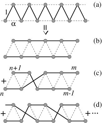
Figure 1: Schematic picture of the ground state of the frustrated $S=1$ chain (1): (a) VBS state with one string corresponding to the Haldane phase; (b)–(d) VBS states with two strings contained in the DH (large-$\alpha$) phase.

There is, however, another order parameter surviving pair creation. One can define double string order as

$${\mathcal{O}}^{a}_{2}(n,m)=\langle S^{a}_{n}S^{a}_{n+1}(\exp\sum_{j=n+2}^{m-2}i\pi S^{a}_{j})S^{a}_{m-1}S^{a}_{m}\rangle,$$ (7)

and it is easy to check that it is not sensitive to the presence of any type of soliton pairs. The corresponding order parameter ${\mathcal{O}}_{2}=\lim_{|m-n|\to\infty}{\mathcal{O}}^{a}_{2}(n,m)$ is finite in any state which is a product of exactly two VBS strings, arbitrarily intertwined, because one can always factorize (7) into a product of two normal SOPs defined along those strings. On the other hand, the correlator (7) decays exponentially in the AKLT state with only one VBS string, because in this case (7) factorizes into $\langle S^{a}_{n}S^{a}_{m}\rangle{\mathcal{O}}_{1}(m-1,n+1)$. One may say that ${\mathcal{O}}_{2}$ measures the connectivity of the state, telling us how many VBS strings are there. It is natural to assume that ${\mathcal{O}}_{2}$ should be the order parameter characterizing the DH phase.

The above assumption is readily confirmed by the DMRG results. In our DMRG calculations, we have considered chains with open boundary conditions and up to $L=300$ spins, keeping $M=400$ states. We have calculated the excitation gap and both the conventional SOP ${\mathcal{O}}_{1}$ and the new SOP ${\mathcal{O}}_{2}$ (see Fig. 2). While the results were converged in the number of states kept, we carried out finite size extrapolation for frustrations very close to the transition point. We observe that both order parameters exclude each other in the sense that if either of them decays to zero, the thermodynamic limit of the other is non-zero and vice versa. The value of ${\mathcal{O}}_{2}$ is strictly zero below $\alpha<0.77$, and for $\alpha=0.775$ already at 0.061, i.e. 44% of its asymptotic value of 0.1401 for $\alpha\rightarrow\infty$, where one has two completely decoupled unfrustrated chains, and ${\mathcal{O}}_{2}$ is simply the square of the string order for the unfrustrated $S=1$ Heisenberg chain, 0.3743. In fact, for the frustration $\alpha=1.3$, it reaches 90% of the asymptotic value. At both sides of the transition, both order parameters exhibit clearly finite values, signalling the first order transition. The finding of a finite gap for all values of $\alpha$ is consistent with this picture.

In order to describe the physical picture sketched above, we have constructed the effective theory based on the soliton states (5). For $\alpha<{3\over 4}$ we regard the AKLT state as the vacuum state, and introduce bosonic operators $t_{nr}^{{\dagger}}$ creating states $|r,n\rangle$, $r=(x,y,z)$. Similarly, for $\alpha>{3\over 4}$ we treat the two-subchain VBS state shown in Fig. 1b as the vacuum; this state can be conveniently represented in the following MP form:

$$\Psi_{AKLT2}=\mbox{tr}\big{\{}\widetilde{\mathcal{G}}_{1}{\mathcal{G}}_{2}\cdots\widetilde{\mathcal{G}}_{N-1}{\mathcal{G}}_{N}\big{\}},$$ (8)

where ${\mathcal{G}}_{n}=(g_{n}\otimes\openone)$ and $\widetilde{\mathcal{G}}_{n}=(\openone\otimes g_{n})$ are $4\times 4$ matrices, and the total number of spins $N$ is assumed to be even. The operators $t_{nr}^{{\dagger}}$ are interpreted as creating soliton states $|\widetilde{r,n}\rangle$ on the subchains, defined by replacing the $n$-th matrix ${\mathcal{G}}_{n}$ or $\widetilde{\mathcal{G}}_{n}$ in (8) with the matrix ${\mathcal{F}}^{r}_{n}=(f^{r}_{n}\otimes\openone)$ or $\widetilde{\mathcal{F}}^{r}_{n}=(\openone\otimes f^{r}_{n})$, respectively.

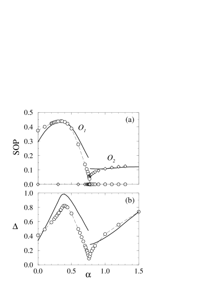
Figure 2: (a) the string order ${\mathcal{O}}_{1}$ and double string order ${\mathcal{O}}_{2}$ as functions of the frustration $\alpha$; (b) the same for the excitation gap $\Delta$. Symbols correspond to the DMRG data, and solid lines are theoretical predictions from the effective model.

Calculating all matrix elements corresponding to the hopping of solitons and creation of pairs, and passing to the momentum representation, one obtains on the quadratic level the effective Hamiltonian of the form

$$\widehat{H}_{eff}=\sum_{kr}A_{k}t^{{\dagger}}_{k,r}t^{\phantom{{\dagger}}}_{k,r}+{1\over 2}B_{k}(t^{{\dagger}}_{k,r}t^{{\dagger}}_{k,r}+\mbox{h.c.}).$$ (9)

Here for the Haldane phase ($\alpha<{3\over 4}$) the amplitudes $A_{k}$, $B_{k}$ are given by the expressions

$$B_{k} = 2(112\alpha/27-1)\cos{k}$$

$$- (10\alpha/9)\cos{2k}-(13\alpha-3)C^{(1,1)}_{k},$$

$$A_{k} = B_{k}+(4/27)\times$$

$$\times \big{\{}15-13\alpha+(9-16\alpha)\cos{k}-3\alpha\cos{2k}\big{\}},$$

and for the DH phase ($\alpha>{3\over 4}$) one has

$$B_{k} = (2/9)(2\cos{k}-\alpha\cos{2k})-C^{(3,2)}_{k}-\alpha C^{(4,2)}_{k}$$

$$A_{k} = B_{k}+(4\alpha/9)(5+3\cos{2k}),$$ (11)

where the following shorthand notation is used:

$$C^{(l^{\prime},l)}_{k}={8\over 9}\,{3\cos{(l^{\prime}k)}+\cos{\big{(}(l-l^{\prime})k\big{)}}\over 5+3\cos{(lk)}}.$$

The Hamiltonian (9) does not take into account any interaction between the solitons. The most important contribution to the interaction comes from the constraint that at most one particle can be present at a given site, which is effectively equivalent to the infinite on-site repulsion $U$. We treat the effect of the constraint using Brueckner’s approximation along the lines proposed by Kotov et al.Kotov+98 . In this approach, one neglects the contribution of anomalous Green’s functions and obtains in the limit $U\to\infty$ the vertex function $\Gamma_{rr^{\prime},ss^{\prime}}=\Gamma(k,\omega)(\delta_{rs}\delta_{r^{\prime}s^{\prime}}+\delta_{rs^{\prime}}\delta_{r^{\prime}s})$, where $k$ and $\hbar\omega$ are respectively the total momentum and energy of the incoming particles, with

$${1\over\Gamma(k,w)}=-{1\over N}\sum_{q}{Z_{q}Z_{k-q}u^{2}_{q}u^{2}_{k-q}\over\omega-\Omega_{q}-\Omega_{k-q}}.$$ (12)

The corresponding normal self-energy $\Sigma(k,\omega)$ is

$$\Sigma(k,\omega)=(4/N)\sum_{q}Z_{q}v_{q}^{2}\Gamma(k+q,\omega-\Omega_{q}).$$ (13)

The normal Green function has the form

$$G(k,\omega)={\omega+A_{k}+\Sigma(-k,-\omega)\over(\omega-\Sigma_{-})^{2}-(A_{k}+\Sigma_{+})^{2}+B_{k}^{2}},$$ (14)

where $\Sigma_{\pm}\equiv{1\over 2}\big{\{}\Sigma(k,\omega)\pm\Sigma(-k,-\omega)\big{\}}$, and its quasiparticle part is given by

$$G(k,\omega)={Z_{k}u_{k}^{2}\over\omega-\Omega_{k}+i\varepsilon}-{Z_{k}v_{k}^{2}\over\omega+\Omega_{k}-i\varepsilon}$$ (15)

which defines the renormalization factors $Z_{k}$, the Bogoliubov coefficients $u_{k}$, $v_{k}$ and the spectrum $\Omega_{k}$ as follows:

$$\Omega_{k} = \Sigma_{-}+E_{k},\quad E_{k}=\{(A_{k}+\Sigma_{+})^{2}-B_{k}^{2}\}^{1/2},$$

$$u_{k}^{2} = {1\over 2}\big{\{}1+(A_{k}+\Sigma_{+})/E_{k}\big{\}},\quad v_{k}^{2}=u_{k}^{2}-1,$$

$${1\over Z_{k}} = 1-{\partial\Sigma_{-}\over\partial\omega}-{(A_{k}+\Sigma_{+})\over E_{k}}\,{\partial\Sigma_{+}\over\partial\omega}$$ (16)

where $\Sigma_{\pm}$ and their derivatives are understood to be taken at $\omega=\Omega_{k}$. The system of equations (12), (13), (Connectivity transition in the frustrated $S=1$ chain revisited) has to be solved self-consistently with respect to $Z$ and $\Sigma$. This approach is valid as long as the soliton density $\rho={3\over N}\sum_{q}Z_{q}v_{q}^{2}$ remains small, ensuring that the contribution of anomalous Green’s functions is irrelevant.Kotov+98

It should be remarked that our Eqs. (Connectivity transition in the frustrated $S=1$ chain revisited) differ from the corresponding expressions of Kotov et al.,Kotov+98 which can be obtained from (Connectivity transition in the frustrated $S=1$ chain revisited) assuming that $\Sigma(k,\omega)$ is almost linear in $\omega$ in the frequency interval $(-\Omega_{k},\Omega_{k})$; however, this latter assumption fails for the present model.

As far as Eqs. (12), (13), (Connectivity transition in the frustrated $S=1$ chain revisited) are solved, one can calculate the reduction of the string order caused by the presence of pairs. For the usual SOP in the Haldane phase ($\alpha<{3\over 4}$) one finds

$${\mathcal{O}}_{1}^{z}=(4/9)(1-2\gamma\rho_{p}R)^{2}.$$ (17)

Here $\gamma={2\over 3}$ is the correcting factor which takes into account that $(zz)$ pairs do not affect ${\mathcal{O}}_{1}^{z}$, and the total density of soliton pairs $\rho_{p}={1\over 2N}\sum_{nn^{\prime}r}\langle t^{{\dagger}}_{nr}t^{{\dagger}}_{n^{\prime}r}\rangle^{2}$ and the mean size of the pair $R$ are given by

$$\rho_{p}=(3/2N)\sum_{q}Z_{q}^{2}u_{q}^{2}v_{q}^{2},$$

$$R={\sum_{m\geq 1}mw_{m}^{2}\over\sum_{m\geq 1}w_{m}^{2}},\quad w_{m}={1\over N}\sum Z_{q}u_{q}v_{q}e^{iqm}.$$ (18)

A similar calculation for ${\mathcal{O}}_{2}$ in the DH phase yields

$${\mathcal{O}}_{2}^{z}=(4/9)^{2}\big{\{}1-\gamma\rho_{p}^{l}R^{l}\big{\}}^{4}\big{\{}1-2\gamma\rho_{p}^{t}R^{t}\big{\}}^{2},$$ (19)

where $\rho_{p}^{l}$ and $\rho_{p}^{t}$ are densities of the “longitudinal” (sitting on a single subchain) and “transversal” (intersubchain) pairs, respectively,

$$\rho_{p}^{l,t} = (\rho_{p}\pm\widetilde{\rho}_{p})/2,$$

$$\widetilde{\rho}_{p} = {3\over 2N}\sum_{q}Z_{q}Z_{q+\pi}(u_{q}v_{q})(u_{q+\pi}v_{q+\pi}),$$ (20)

and $R^{l}$, $R_{t}$ are the corresponding average pair sizes (note that all distances are defined in terms of the initial chain):

$$R^{l}={\sum_{m\geq 1}(2m)w_{2m}^{2}\over\sum_{m\geq 1}w_{2m}^{2}},\quad R^{t}={\sum_{m\geq 0}(2m)w_{2m+1}^{2}\over\sum_{m\geq 0}w_{2m+1}^{2}}.$$ (21)

In Fig. 2 we show the results of the DMRG calculations together with the theoretical curves obtained on the basis of the effective theory. Though the theoretical calculations are not quantitatively satisfactory, they nevertheless capture the essential behavior of the system. In the vicinity of the transition the theoretical results are rather far from the numerical data; one reason is that at $\alpha={3\over 4}$ the completely dimerized state has the same variational energy as the VBS states in Fig. 1(a,b), which is not taken into account in the theory.

It should be mentioned that a definition similar to (7) was recently used by Todo et al.Todo+01 for the spin-1 ladder, with $(n,n+1)$ and $(m-1,m)$ placed on two rungs. They have shown that such an order is present in the $S=1$ ladder for any ratio of the rung and leg exchange. One may thus expect that in the frustrated $S=1$ chain with alternating nearest-neighbor interaction the DH phase is smoothly connected to the dimerized phase. However, this problem is not clear since in a ladder there are three ways to define the double string order, depending on whether the initial and final pairs of points are placed on the rungs or diagonals, and only one of the definitions gives a finite value in the completely dimerized state.

In summary, we have identified the nature of the first order transition in the frustrated $S=1$ chain as a change in the connectivity of underlying VBS states, and established the proper order parameter for the large-$\alpha$ phase. We have also developed the effective description based on soliton states, which qualitatively describes the physics of both phases.

A.K. gratefully acknowledges the hospitality of the Institute for Theoretical Physics, Hannover, where the present study was initiated. This work is supported in part by the grant I/75895 from the Volkswagen-Stiftung. U.Sch. is supported by a Gerhard-Hess prize of the DFG.

References

- (1) H. T. Diep (ed.), Magnetic Systems with Competing Interactions (Frustrated Spin Systems), World Scientific, Singapore, 1994.
- (2) M. den Nijs and K. Rommelse, Phys. Rev. B 40, 4709 (1989); S.M. Girvin, D.P. Arovas, Phys. Scr. T 27, 156 (1989); T. Kennedy, H. Tasaki, Phys. Rev. 45, 304 (1992).
- (3) T. Kennedy, J. Phys.: Cond. Matter 2, 5737 (1990).
- (4) I. Affleck, T. Kennedy, E.H. Lieb, H. Tasaki, Phys. Rev. Lett. 59, 799 (1987); Commun. Math. Phys. 115, 477 (1988).
- (5) A. Kolezhuk, R. Roth, and U. Schollwöck, Phys. Rev. Lett. 77, 5142 (1996); Phys. Rev. B 55, 8928 (1997).
- (6) T. Hikihara, M. Kaburagi, H. Kawamura, and T. Tonegawa, J. Phys. Soc. Jpn. 69, 259 (2000).
- (7) M. Fannes, B. Nachtergaele and R. F. Werner, Europhys. Lett. 10, 633 (1989); Commun. Math. Phys. 144, 443 (1992).
- (8) A. Klümper, A. Schadschneider and J. Zittartz, J. Phys. A 24, L955 (1991); Z. Phys. B 87, 281 (1992); Europhys. Lett. 24, 293 (1993).
- (9) G. Fáth and J. Sólyom, J. Phys.: Cond. Matter 5, 8983 (1993); U. Neugebauer and H.-J. Mikeska, Z. Phys. B 99, 151 (1996).
- (10) V. N. Kotov, O. Sushkov, Zheng Weihong, and J. Oitmaa, Phys. Rev. Lett. 80, 5790 (1998).
- (11) S. Todo, M. Matsumoto, C. Yasuda, and Hajime Takayama, eprint cond-mat/0106073.