Abstract

We consider a deformable body immersed in an incompressible liquid that is randomly stirred. Sticking to physical situations in which the body departs only slightly from its spherical shape, we calculate the mean squared displacement and the diffusion constant of the body. We give explicitly the dependence of the diffusion constant on the velocity correlations in the liquid and on the size of the body. We emphasize the particular case in which the random velocity field follows from thermal agitation.

I Introduction

Systems of deformable objects immersed in a liquid are very common in every day life. Milk and blood, for example, are such composite systems. Milk can be viewed as an emulsion of fat globules in water while blood is a suspension of cells ( that have some rigidity) in water. The physical description of the set of objects present in a given liquid involves the location of the objects, their shape and in some cases the strains on the objects or any other fields that are needed to describe the objects in addition to their location and shape. The actual solution of such systems is extremely difficult because each object interacts with itself and with the other objects via hydrodynamic interactions. Hence, we are facing a many body problem with the additional complication, that each object is not described by a single degree of freedom ( its center of mass) but actually by an infinite number of degrees of freedom, where all the deformation degrees of freedom, corresponding to all the objects, interact. The situation is simplified a little if the deviation of the objects from spherical shape remains small [1, 2]. This happens when the agitation of the host liquid is not too strong and when the density of the objects is not too high ( Close packing would cause finite deformations, although perhaps still treatable within the small deformation approximation). Our final goal is to obtain the response of the composite system to a given velocity field imposed on the liquid. The velocity field we have in mind may be fixed in time like simple shear or randomly fluctuating in time and space. Even in the first case the velocity field experienced by each object separately must have a random part due to the random passage of other objects near by. The present article is the first in a series that deals with this general problem and it concentrates, within the small deformation approximation, on the diffusion of the center of mass of a deformable body in the presence of a random external velocity field, imposed on the liquid. It is possible to consider the center of mass separately from the deformation degrees of freedom, that will be discussed in a future publication, because as will be shown in the following, they are decoupled in the small deformation approximation. We study the mean square displacement (MSD) of an object as a function of time for a general random velocity field that has given correlations in space and time. For long periods of time the MSD is usually linear in time, enabling us to discuss it in terms of a diffusion constant that depends on the size of the object, $R$, and the correlations present in the liquid. There are, of course, cases where the MSD does not behave linearly at long times and the method we develop here is quite capable of dealing with those cases too. Our main concern is in objects in which the state of lowest energy is of spherical shape. This is the case for deformable objects dominated by surface tension [3]. Our results results concerning the motion of the center of the object will hold also for cases where the shape of lowest energy is nearly spherical (for example a body with bending energy [4, 5] and spontaneous curvature close to that of a sphere with the same volume).

The paper is organized in the following way: In section II we define the system under consideration, discuss its properties, and construct the basic equations. In section III we derive the equation of motion for the center and the MSD in integral and differential forms. In section IV we discuss the results and demonstrate their use for different kinds of noise realizations. The specific case of thermal agitation is considered in section V. In appendix A, we construct the velocity correlations for the case of thermal agitation and in appendix B we consider the physical conditions under which the small deformation approximation is valid.

II The System

Consider a single deformable body immersed in a host fluid. The system is chosen to have the following characteristics:

1. The host fluid is incompressible, $\vec{\nabla}\cdot\vec{v}=0$. In addition, we assume that the Reynolds number is small so that the Stokes approximation is applicable.

2. The body is characterized by an energy that depends on its shape. The shape of minimum energy is a sphere. The shape of the surface of the body is described by the equation: $\psi(\vec{r})=0$ where $\psi(\vec{r})$ is a scalar three dimensional field (Fig. 1).( Although our derivation considers only objects for which the shape of minimum energy is a sphere, all the conclusions concerning the MSD carry over to cases where the shape of minimum energy is nearly spherical).

3. A deformation of the body induces a force density on the host fluid. As a result, the fluid’s velocity is given by the sum of $\vec{v}_{ext}$, which is caused by external sources, and $\vec{v}_{\psi}$, which is induced by the body.

4. The external velocity, $\vec{v}_{ext}$, is random and is chosen to have zero average and known correlations. It is convenient to define the external velocity in terms of its spatial Fourier transform as

   $$v_{ext_{i}}(\vec{q}\ )\equiv\sum_{j}\left(\delta_{ij}-\frac{q_{i}q_{j}}{q^{2}}\right)u_{j}(\vec{q}),$$ (1)

   where $\vec{u}(\vec{q})$ is a general vector field and the subscripts denote Cartesian components. This definition implies only that the fluid is incompressible and in any other way is general. Next, invariance under translations in space and time and under rotations yields the form of the correlations of the velocity,

   $$\left\langle u_{l}(\vec{q},t)\right\rangle=0\mbox{ and }$$ (2)

   $$\left\langle u_{l}(\vec{q},t_{1})u_{m}(\vec{p},t_{2})\right\rangle=\delta_{lm}\delta(\vec{q}+\vec{p})\phi(q,|t_{2}-t_{1}|),$$ (3)

   where $\delta_{lm}$ is the Kronecker delta and $\delta()$ is the Dirac delta function and $\phi$ is a general function of $q$ and $|t_{2}-t_{1}|$. If the random velocity field is characterized by a length scale and a characteristic time scale then it is convenient to write it as $\phi(\xi q,|t_{2}-t_{1}|/\tau)$, where $\xi$ and $\tau$ are, respectively, the correlation length and the memory time scale of the external velocity .

5. The surface elements of the body are carried by the host fluid [6], i.e. each surface point moves according to

   $$\dot{\vec{r}}=\vec{v}_{ext}(\vec{r})+\vec{v}_{\psi}(\vec{r}).$$ (4)

6. We assume that the external velocity is weak enough to cause only minor shape fluctuations of the body.
   

We will be interested in the following in the Mean Squared Displacement (MSD) of the center. Since the body is deformable the definition of its center is not unique. For periods of time shorter than $\tau$ the result depends on the definition of the center. It turns out, however, that the value of the MSD at longer times does not depend on the specific choice, because for long times the MSD (according to any reasonable definition) is much larger than the size of the body. Therefore, the results for the diffusion constant are general and do not depend on the specific definition of the center which will be determined later.In cases where the long time dependence of the MSD is not linear, it is still tending to infinity with time, so that again the specific definition of the center does not matter.

Following the line of derivation of Schwartz and Edwards [6, 7], equation (4) may be turned into a continuity equation for $\psi$,

$$\frac{\partial\psi}{\partial t}+(\vec{v}_{ext}+\vec{v}_{\psi})\cdot\vec{\nabla}\psi=0.$$ (5)

Consider a deformable body, carried by the host fluid in such a way that at any instant it is nearly spherical. Its state can thus be characterized by the position of its center, $\vec{r}_{0}(t)$, and a deformation function $f(\Omega,t)$ that describes the shape by the equation

$$\psi(\vec{r},t)\equiv\frac{\rho}{R}+f(\Omega,t)-1=0,$$ (6)

where $\rho\equiv|\vec{r}-\vec{r}_{0}|$ is the distance of the surface from the center in the direction of the solid angle $\Omega$ and $R$ is the radius of the body when not deformed. The deformation function $f$ can be expanded in spherical harmonics, $f(\Omega,t)=\sum_{l=0}^{\infty}\sum_{m=-l}^{l}f_{l,m}(t)Y_{l,m}(\Omega)$. The center of the shape, $\vec{r}_{0}(t)$, is defined as that point around which $f_{1m}(t)=0$.
Equations (5) and (6) lead to a linear equation for each $f_{l,m}$,

$$\frac{\partial f_{lm}}{\partial t}+\lambda_{l}f_{lm}+\frac{1}{R}[\hat{\rho}\cdot(\vec{v}_{ext}-\dot{\vec{r}}_{0})]_{lm}=0,$$ (7)

where $\hat{\rho}$ is a unit vector directed outwards from the center in the direction of $\Omega$, and

$$[\hat{\rho}\cdot(\vec{v}_{ext}-\dot{\vec{r}}_{0})]_{lm}=\int d\Omega\left\{\hat{\rho}\cdot\left[\vec{v}_{ext}(\vec{r}_{0}+R(1-f)\hat{\rho})-\dot{\vec{r}}_{0}\right]Y^{*}_{l,m}(\Omega)\right\}.$$ (8)

The eigenvalues $\lambda_{l}$’s characterize the decay of a slightly deformed sphere into a sphere in the absence of the external velocity. Different physical systems are characterized by different sets of $\lambda_{l}$’s. However, it is obvious that the decay must depend only on $l$ because of the spherical symmetry. Examples of systems for which different sets of $\lambda_{l}$ have been calculated include: a droplet with a surface tension and equal viscosities inside and outside [7] and a droplet with surface tension for a viscosity much higher inside the droplet than outside [8]. Other systems for which the following results are applicable to, in the small deformations approximation, include a droplet with a bending energy [9], a droplet with a bending energy and in-plane dissipation [10] and a droplet with both surface tension and bending energy [11]. Our following discussion is therefore general and not limited to one specific system.

III Derivation of the MSD

Equation (7) implies that in order that $f_{1,m}$ stays zero for all times we must have as an equation determining the location of the center

$$[\hat{\rho}\cdot(\vec{v}_{ext}-\dot{\vec{r}}_{0})]_{1m}=0\ \ ,\ m=-1,0,1.$$ (9)

For $l\neq 1$ it is clear that $\dot{\vec{r}}_{0}$ can be dropped from the last term on the left hand side of Eq. (7). Therefore $f(\Omega,t)$ is linear in $\vec{v}_{ext}$ (for long enough times the initial deformations have already decayed). Consequently we can always drop, for small enough $\vec{v}_{ext}$, $f$ in the argument of $\vec{v}_{ext}$ on the right hand side of Eq. (8) (The physical conditions for which this approximation is valid are discussed in appendix B). This results in decoupling of the deformation degrees of freedom from that of the center of the sphere. The equation for the motion of the center can thus be given, using linear combinations of $Y_{1,m}$, in vector form as

$$\int d\Omega\ \hat{\rho}\ \left(\hat{\rho}\cdot\dot{\vec{r}}_{0}\right)=\int d\Omega\ \hat{\rho}\ \left(\hat{\rho}\cdot\vec{v}_{ext}(\vec{r}_{0}+R\hat{\rho})\right).$$ (10)

We integrate the left hand side of the above and express the external velocity in terms of its Fourier transform on the right hand side to obtain

$$\frac{4\pi}{3}\dot{\vec{r}}_{0}=\int d\Omega\int d^{3}q\ \hat{\rho}\left(\hat{\rho}\cdot\vec{v}_{ext}(\vec{q},t)\right)e^{-i\vec{q}\cdot(\vec{r}_{0}+R\hat{\rho})}.$$ (11)

We use the partial waves expansion [12, 13]:

$$e^{-i\vec{q}\cdot(R\hat{\rho})}=\sum_{l=0}^{\infty}\sum_{m=-l}^{l}(-i)^{l}4\pi j_{l}(qR)Y_{lm}^{*}(\Omega_{q})Y_{lm}(\Omega),$$ (12)

where $\Omega$ and $\Omega_{q}$ are the solid angles in the directions of $\hat{\rho}$ and $\vec{q}$ respectively and $j_{l}$ is the spherical Bessel function of order $l$. We integrate over $\Omega$ and obtain

$$\dot{\vec{r}}_{0} = 3\int d\vec{q}e^{-i\vec{q}\cdot\vec{r}_{0}}\left(\frac{1}{3}j_{0}(qR)+j_{2}(qR){\bf A}\right)\vec{v}_{ext}(\vec{q},t).$$ (13)

The matrix ${\bf A}(\vec{q})$ is given by

$$A_{ij}=-\frac{2}{3}\delta_{ij}+\left(\delta_{ij}-\frac{q_{i}q_{j}}{q^{2}}\right).$$ (14)

It may seem that ${\bf A}$ on the right hand side of Eq. (13) mixes directions. However, the bracketed term in Eq. (14) is just a projection operator on the transverse direction. The external velocity is incompressible and hence already transverse. Consequently, this term acts as a unity operator, $\delta_{ij}$, and Eq. (13) leads to

$$\dot{\vec{r}}_{0} = \int d\vec{q}e^{-i\vec{q}\cdot\vec{r}_{0}}\left(j_{0}(qR)+j_{2}(qR)\right)\vec{v}_{ext}(\vec{q},t).$$ (15)

Equation (15) is the explicit equation of motion for the center of the body. In the limit $R\rightarrow 0$ the approximation, $\dot{\vec{r}}_{0}=\vec{v}_{ext}(\vec{r}_{0},t)$ is obtained. Note that this equation is general and describes the motion of the center for any given (small enough) external velocity field.

Next, we calculate the MSD, $\langle\left(\Delta\vec{r}_{0}\right)^{2}\rangle$, as a function of the elapsed time, $t$. Consider a specific realization of the external velocity field.

The Displacement of the center is given by the trivial equation

$$\Delta\vec{r}_{0}(t)=\int_{0}^{t}\dot{\vec{r}}_{0}(t^{\prime})dt^{\prime}.$$ (16)

Hence, the MSD is given by

$$\left\langle\left(\Delta\vec{r}_{0}(t)\right)^{2}\right\rangle=\int_{0}^{t}dt_{1}\int_{0}^{t}dt_{2}\ \left\langle\dot{\vec{r}}_{0}(t_{1})\cdot\dot{\vec{r}}_{0}(t_{2})\right\rangle.$$ (17)

The correlations of the external velocity given in $q$ space are obtained from Eq.(1) and (3) . Assuming the decomposition [14, 15]

$$\left\langle v_{ext_{i}}(\vec{q}_{1},t_{1})v_{ext_{j}}(\vec{q}_{2},t_{2})e^{-i\vec{q_{1}}\cdot\vec{r}_{0}(t_{1})}e^{-i\vec{q_{2}}\cdot\vec{r}_{0}(t_{2})}\right.\left.\right\rangle=$$ (18)

$$\left\langle v_{ext_{i}}(\vec{q}_{1},t_{1})\right.\left.v_{ext_{j}}(\vec{q}_{2},t_{2})\right\rangle\left\langle e^{-i\vec{q_{1}}\cdot\vec{r}_{0}(t_{1})}e^{-i\vec{q_{2}}\cdot\vec{r}_{0}(t_{2})}\right\rangle$$ (19)

and in addition that the distribution of $\Delta\vec{r}_{0}(t)$ is Gaussian, i.e.

$$\left\langle e^{-i\vec{q}\cdot\Delta\vec{r}_{0}(t)}\right\rangle=e^{-\frac{q^{2}}{6}\left\langle(\Delta r_{0}(t))^{2}\right\rangle},$$ (20)

we obtain

$$\left\langle\left(\Delta\vec{r}_{0}(t)\right)^{2}\right\rangle= \int_{0}^{t}dt_{1}\int_{0}^{t}dt_{2}\int d\vec{q}e^{-\frac{q^{2}}{6}\left\langle\left(\vec{r}_{0}(t_{1})-\vec{r}_{0}(t_{2})\right)^{2}\right\rangle}$$ (22)

$$\left(j_{0}(qR)+j_{2}(qR)\right)^{2}\sum_{i}\left(1-\frac{q_{i}^{2}}{q^{2}}\right)\phi(q,|t_{2}-t_{1}|).$$

The only term that depends on angel is $1-q_{i}^{2}/q^{2}$. Performing the angular integration $\int d\Omega_{q}\left(1-q_{i}^{2}/q^{2}\right)=8\pi/3$, and summing up the three terms we obtain, denoting the MSD by $F(t)$,

$$F(t)=16\pi\int_{0}^{t}dt^{\prime}\int_{0}^{\infty}q^{2}dqe^{-\frac{q^{2}}{6}F(t^{\prime})}\phi(q,t^{\prime})\left(j_{0}(qR)+j_{2}(qR)\right)^{2}(t-t^{\prime}).$$ (23)

Eq. (23) can be turned also to a differential equation. Differentiating Eq. (23) twice we obtain

$$\ddot{F}(t)=16\pi\int_{0}^{\infty}q^{2}dqe^{-\frac{q^{2}}{6}F(t)}\phi(q,t)\left(j_{0}(qR)+j_{2}(qR)\right)^{2}.$$ (24)

The initial conditions are

$$F(0)=0$$ (25)

and

$$\dot{F}(0)=0.$$ (26)

The latter condition is valid in cases where the correlation function, $\phi(q,t)$, is finite at $t=0$. The only exception is the case of white noise, where one must carefully check the result of the first differentiation and determine $\dot{F}(0)$. (Actually (26) is always correct, because any noise that is of physical origin must be correlated in time. The widely used white noise is just a very useful idealization of the real situation, that will result in $\dot{F}(0)=0$ and $\dot{F}(\delta)$ having a value that is not small for rather small $\delta$’s). The advantage of the differential form is that its numerical solution can be easily obtained by advancing $F(t)$ in time. Note that equation (24) above is not restricted to cases that can be described in terms of a diffusion constant.

IV Properties of the MSD

The random velocity field may be caused by thermal agitation which is an equilibrium phenomenon or by non-equilibrium process such as mechanical stirring. While Eq. (24) can supply, by numerical solution, the MSD for any velocity correlation, there are families of velocity correlations in which at least part of the solution of (24) or (23) can be obtained analytically, rendering the process of solving for the MSD much easier. The simplest case is where the correlations are white in time, namely $\phi(q,t)=\tilde{\phi}(q)\delta(t)$. In those cases $F(t)$ is linear at all times, $F(t)\equiv 3Dt$, where $D$ is the diffusion constant and Eq. (23) that is an equation for the function $F(t)$ is replaced by an explicit expression for the diffusion constant

$$D=\frac{8\pi}{3}\int_{0}^{\infty}q^{2}\ dq\ \tilde{\phi}(q)(j_{0}(qR)+j_{2}(qR))^{2}.$$ (27)

A family of correlations that is a simple extension of the above, where it is quite easy to see what is happening, is defined by $\phi(q,t)=\tilde{\phi}(q)\tilde{G}(\frac{t}{\tau})$, were $\tilde{G}$ is a function that decays when its argument becomes of order 1. It is clear from Eq. (26) that for short times the MSD must behave as $t^{2}$ while for long times it must be linear in $t$, since for $t>>\tau$ the time dependence cannot be distinguished from white noise. The function $\tilde{\phi}(q)$, will naturally have a cut-off factor $g(q\xi)$, where $\xi$ is the correlation length. Clearly, the correlation length cannot be expected to be smaller than the distance between the particles of which the fluid is composed and not larger than the size of the system.

The MSD depends, of course, on the ratio $\gamma=\frac{R}{\xi}$. Generally speaking, as $\gamma$ increases the slope of the MSD and particularly the diffusion constant decreases. This is due to the fact that as $\gamma$ increases, different regions of the surface become less correlated and move in different directions. In the limit $\gamma\rightarrow\infty$, the movement of the center ceases and $F(t)$ is always zero. In the limit $\gamma\rightarrow 0$, the bracketed Bessel term in Eq. (23) and (24) can be replaced by unity (since $\lim_{qR\rightarrow 0}\left(j_{0}(qR)+j_{2}(qR)\right)=1$). A close inspection of the derivation reveals that this limit produces the same MSD equation as the equation for the approximation $\dot{\vec{r}}_{0}=\vec{v}_{ext}(\vec{r}_{0})$. I.e. the latter approximation is accurate for an infinite correlation length, or point particles.

In the following we will consider the dependence of the diffusion constant on the size of the object $R$. Consider a correlation such as $\phi(q,t)=C\ \delta(t)\ (q\xi)^{\alpha}g(q\xi)$, where $g$ is a cutoff function and $g(0)>0$. Note that as discussed above the results that will be obtained here for the diffusion constant hold true also for a finite correlation time. We insert the above correlation function into equation (23), then substitute $qR$ with $u$, and obtain

$$D=\frac{8\pi C\xi^{\alpha}}{3R^{3+\alpha}}\int_{0}^{\infty}du\ u^{2+\alpha}g(\frac{\xi}{R}u)[j_{0}(u)+j_{2}(u)]^{2}.$$ (28)

In the limit $R/\xi\rightarrow\infty$ we distinguish between two cases: $\alpha<1$ and $\alpha>1$. Since the large $u$ dependence of $j_{0}(u)+j_{2}(u)$ is proportional to $cos(u)/u^{2}$ we find that

$$D\propto\left\{\begin{array}[]{ll}\frac{C\xi^{\alpha}}{R^{3+\alpha}}&$for $\alpha<1\\ \frac{C\xi}{R^{4}}&$for $\alpha>1.\\ \end{array}\right.$$ (31)

In the opposite limit $R/\xi\rightarrow 0$ we find that regardless of $\alpha$

$$D\propto\frac{C}{\xi^{3}}.$$ (32)

(Note here that we have written the power law dependence of $\phi(q)$ as $q^{\alpha}\xi^{\alpha}$ but having other dimensional constants in the model may make $C$ depend on $\xi$, so that Eqs. (31) and (32) may be considered only as equations that yield the dependence of $D$ on the radius $R$).

The dependence of the diffusion constant on the decay time scale can be also deduced when the correlation function is separable (i.e. the second family). Using simple dimensional analysis, Eq. (23) leads to the conclusion that the diffusion constant is linear in $\tau$ ( in addition to the possible dependence of $C$ on $\tau$): $D\sim C\tau$.

There is another class of velocity correlations that is not separable but allows the calculation of the long time behavior of the MSD. This class is defined by a scaling form of the velocity correlations,

$$\phi(q,t)=Cq^{-\alpha}f\left(\Gamma qt^{\beta}\right),$$ (33)

where $\Gamma$ and $C$ are dimensional constants, $f$ is a function with a finite decay length and $\alpha<3$. The solution is obtained by assuming that $F(t)=At^{\nu}$. The integrand in Eq. (24) has in it two functions, each cutting the integral off at different value of $q$ that is a function of t. The dominant cut-off at large times $t$, is the one that cuts the integrand off at smaller $q$’s. What remains is just a scaling argument that leads from Eq. (24) to the following result:

$$\nu=\left\{\begin{array}[]{ll}\tilde{\nu}&$if $\tilde{\nu}>1\\ 1&$if $\tilde{\nu}\leq 1\\ \end{array}\right.,$$ (36)

where

$$\tilde{\nu}=\left\{\begin{array}[]{ll}4/(5-\alpha)&$if $\tilde{\nu}>2\beta\\ 2+(\alpha-3)\beta&$if $\tilde{\nu}\leq 2\beta\\ \end{array}\right..$$ (39)

Note that Eq. (36) results from the fact that even if $\ddot{F}(t)=0$ for large $t$ the leading behavior of $F(t)$ is still linear. Note also that in Eq. (39) the two options have to be evaluated first in order to check which of the conditions applies. An explicit equation for the prefactor $A$ can also be easily obtained. We solved Eq. (24) numerically with $\alpha=5/3$ and $\beta=3/5$. The long time dependence of $F(t)$ is depicted in Fig. (4). We see that the long time dependence is given by $F(t)\propto t^{1.2}$, which is exactly the result predicted by Eq. (39). (Note that in this case $\tilde{\nu}=2\beta$).

V Thermal Agitation

Of particular interest is the case where the fluctuations in the velocity field are due to thermal agitation. We describe the effect of temperature by a scalar potential $\varphi$ and a vector potential $\vec{A}$, that fluctuate, have zero average and local correlations in space and time. Both give rise to a force density field

$$\vec{F}=-\vec{\nabla}\varphi+\vec{\nabla}\times\vec{A},$$ (40)

that generates in its turn the fluctuating velocity field in the liquid. Since the velocity field is divergence-less, the scalar potential affects only pressure. Hence, the Fourier transform of the velocity field is given within the Stokes approximation by

$$\vec{v}(\vec{q},t)=\frac{i\vec{q}\times\vec{A}(\vec{q},t)}{\eta q^{2}},$$ (41)

where $\eta$ is the viscosity of the liquid. Since the correlations of $\vec{A}(\vec{r},t)$ are local in space and time, it follows that $\tilde{\phi}(q)$, defined by Eq. (3), is given by

$$\tilde{\phi}(q)=\frac{c}{q^{2}},$$ (42)

where $c$ is a dimensional constant. Dimensional analysis reveals that $c$ must be proportional to $K_{B}T/\eta$ (with a dimensionless proportionality constant). A detailed calculation yields a proportionality constant equal to $(2\pi)^{-3}$ (see appendix A). The final conclusion is that for $R$ larger than the inter-particle distance in the liquid [16],

$$D=\frac{K_{B}T}{5\pi\eta R}.$$ (43)

Note that this result, for a liquid membrane that has liquid inside as well as outside, is different from the stokes result for a hard sphere. (We may expect Eq. (42) to hold only for $q<1/\xi$ where $\xi$ is the inter-particle distance in the liquid but since $R$ is expected to be very large compared to $\xi$, we are always in the situation described by Eq. (31) with $\alpha=-2$). The latter result is similar to the result for a polymer subjected to thermal fluctuations [17] (with a different pre-factor).

A Velocity Correlations for Thermal Agitation

We wish to determine the exact form of the velocity correlation function for the case of thermal agitation. Consider a system in which the random velocity field results from thermal agitation. The transversal part of the linearized Navier-Stokes equation reads:

$$\frac{\partial v_{q}^{i}}{\partial t}=-\nu q^{2}v_{q}^{i}+\frac{F^{i}}{\rho m},$$ (A1)

where $\vec{v}_{q}$ is the Fourier Transform (FT) of the velocity field, $\nu$ is the kinematic viscosity, $\vec{F}$ is the FT of the force density in the liquid, $\rho$ is the number density of the particles and $m$ is the mass of a liquid particle.
We solve this equation under the condition that the force density is white noise in time and obtain,

$$\left\langle v^{i}_{q}(t_{1})v^{j}_{p}(t_{2})\right\rangle=e^{-\nu q^{2}|t_{2}-t_{1}|}\left\langle v^{i}_{q}v^{j}_{p}\right\rangle_{eq},$$ (A2)

where the last average on the right hand side is an equal time average. It is clear from the above that the velocities at different times are correlated, as opposed to white noise. It is possible however to consider effective white noise correlations by integrating the right hand side of (A2) over time and replacing then the decay function $exp(-\nu q^{2}|t_{2}-t_{1}|)$ by some $a(q)\delta(t_{2}-t_{1})$, that will produce the same integral. This yields for the effective white noise velocity field,

$$\left\langle u_{i}(\vec{q},t_{1})u_{j}(\vec{p},t_{2})\right\rangle=\frac{2}{\nu q^{2}}\delta(t_{2}-t_{1})\left\langle v^{i}_{q}v^{j}_{p}\right\rangle_{eq},$$ (A3)

where we denote the effective velocity field by $\vec{u}$ and the real one by $\vec{v}$. $\left\langle v^{i}_{q}v^{j}_{p}\right\rangle$ must be proportional to $\delta(\vec{p}+\vec{q})$ because of invariance to translations and to $[\delta_{ij}-\frac{q_{i}q_{j}}{q^{2}}]$ because of incompressibility. Comparing with Eq. (42), we conclude that there is no additional dependence on $q$.
Therefore,

$$\left\langle v^{i}_{q}v^{j}_{p}\right\rangle=c^{\prime}\delta(t_{2}-t_{1})[\delta{ij}-\frac{q_{i}q_{j}}{q^{2}}].$$ (A4)

Now, we wish to relate the velocity to temperature. Considering that our continuous liquid is actually made up of $N$ discrete particles each having a mass $m$, we know that the total kinematic energy of the liquid is $3N\frac{K_{B}T}{2}$ and as a result we find

$$\left\langle v^{2}(\vec{r})\right\rangle=\frac{3K_{B}T}{m}.$$ (A5)

Expressing $\vec{v}$ in terms of its FT and integrating while keeping in mind that the number of degrees of freedom should be conserved and equal to $3N$ yields

$$c^{\prime}=\frac{K_{B}T}{2m\rho(2\pi)^{3}}$$ (A6)

from which we can see that

$$c=\frac{K_{B}T}{\eta(2\pi)^{3}},$$ (A7)

and the full correlation function reads

$$\left\langle u_{i}(\vec{q},t_{1})u_{j}(\vec{p},t_{2})\right\rangle=\frac{K_{B}T}{\eta(2\pi)^{3}}\delta(\vec{p}+\vec{q})\delta(t_{2}-t_{1})[\delta_{ij}-\frac{q_{i}q_{j}}{q^{2}}]\frac{1}{q^{2}}.$$ (A8)

B Validity of the Small Deformation Approximation

The validity of equation (23) is limited by the approximation of replacing $\vec{v}_{ext}(\vec{r}_{0}+R(1+f)\hat{\rho})$ by $\vec{v}_{ext}(\vec{r}_{0}+R\hat{\rho})$ that has been discussed in section III. The approximation implies that we can, in the limit of small deformations, replace the velocity at the surface with the velocity on the undeformed sphere. To check the approximation, we expand equation (9) to the first nontrivial order in $f$,

$$\int d\Omega Y_{1,m}^{*}(\Omega)\hat{\rho}\cdot[\vec{v}_{ext}(\vec{r}_{0}+R\hat{\rho})+Rf(\Omega,t)\left(\hat{\rho}\cdot\vec{\nabla}\right)\vec{v}_{ext}(\vec{r}_{0}+R\hat{\rho})-\dot{\vec{r}}_{0}]=0.\ \ \$$ (B1)

The approximation is justified if the first order term is negligible with respect to the zeroth order term. A careful inspection reveals that this condition holds if

$$Rf(\Omega,t)<<\xi,$$ (B2)

for any spatial angle $\Omega$ at any instant of time. The following argument is somewhat more intuitive. The deformation of the body is of the size $Rf$, and the external velocity changes at length-scales that are comparable with the correlation length $\xi$. If the deformation is smaller than the correlation length (Fig. 5-A) the external velocity does not change on the length-scale of the deformation, and the approximation is valid. On the other hand, if the correlation length is shorter than the deformation length-scale (Fig. 5-B) the external velocities on the sphere and on the body are uncorrelated, and the approximation is unjustified.
We turn to evaluate $f$. When $R<<\xi$ it is clear that $f$ can be made small by having $V_{ext}$ small enough so that indeed $Rf<<\xi$. The more interesting case is $R/\xi>1$. The deformation $f$ is determined by Eq. (7)

$$\dot{f}_{l,m}+\lambda_{l}f_{l,m}+Q_{l,m}=0,$$ (B3)

where $Q_{l,m}\equiv\frac{1}{R}[\hat{\rho}\cdot\vec{v}_{ext}]_{lm}$. Clearly,

$$|Q_{lm}|<\frac{4\pi}{R}\langle|Y_{lm}|\rangle v_{ext},$$ (B4)

where $v_{ext}$ is the typical magnitude of the external velocity. The average of the spherical harmonic is bound and of order one and therefore can be dropped off. $\lambda_{l}f_{l,m}$ is comparable with $Q_{l,m}$ (eq. B3), therefore, in order that $Rf<<\xi$ we must have $v_{ext}<\lambda_{l}\xi$. A condition that must be true for all values of $l$ and especially for the smallest $\lambda_{l}$ denoted $\lambda_{l\ min}$. Therefore,

$$v_{ext}<\lambda_{l\ min}\xi$$ (B5)

In most cases, however, we can find a stronger condition for the validity of the small deformation approximation. We expect $Q_{l,m}$ to decline as the squared root of the number of independent surface elements, i.e. as $\xi/R$, so that $\lambda_{l}f_{l,m}\sim\frac{v_{ext}}{R}\frac{\xi}{R}$. Therefore the condition, eq.(B2), implies that $v_{ext}<\lambda_{l}R$. Therefore,

$$v_{ext}<\lambda_{l\ min}R.$$ (B6)

Both conditions can be easily maintained in a viscous fluid. The above conditions are general and depend on the specific system via $\lambda_{l}$. For example for a droplet with a surface tension energy and equal viscosities inside and outside, the minimal eigenvalue is $\lambda_{2}=\frac{16}{35}\frac{\lambda}{\eta R}$ [7] (where $\lambda$ is the surface tension constant and $\eta$ is the viscosity) and the condition is $v_{ext}<\frac{16}{35}\frac{\lambda}{\eta}$, while for a viscosity much larger inside $\lambda_{l\ min}=\lambda_{2}=\frac{1}{2}\frac{\lambda}{\eta R}$ [8] and $v_{ext}<\frac{1}{2}\frac{\lambda}{\eta}$ where $\eta$ is the viscosity inside the droplet.

Figure captions

Fig. 1
The deformable body is described by a three dimensional scalar field $\psi(\vec{r})$. The interior is the region where $\psi<0$, the exterior is the region where $\psi>0$ and the outer surface of the body is the locus of the points obeying $\psi(\vec{r})=0$.

Fig. 2
The MSD for a fluid with a memory time scale. $F_{0}\equiv\frac{C\tau^{2}}{\xi^{3}}$.

Fig. 3
The Diffusion constant for typical separable random velocity correlations. $D_{0}\equiv\frac{C\tau}{\xi^{3}}$.

Fig. 4
The MSD for typical non-separable random velocity correlations with the scaling form, $\phi(q,t)=Cq^{-\alpha}exp\left(-\Gamma qt^{\beta}\right)$, where we choose $\alpha=\frac{5}{3}$ and $\beta=\frac{3}{5}$. The MSD depends on the two non-dimensional variables: $\left(\frac{\Gamma}{R}\right)^{\frac{1}{\beta}}t$ and $\mu=CR^{\alpha-5+\frac{2}{\beta}}\Gamma^{-\frac{2}{\beta}}$. The MSD scales for long times as $t^{\frac{6}{5}}$ in agreement with our scaling argument.

Fig. 5
The validity condition for the approximation. Fig. A: The deformation is negligible in respect to the velocity correlation length. Therefore the approximation holds. Fig. B: The deformation length is longer than the correlation length. The velocities on the surfaces of the sphere and droplet are uncorrelated.

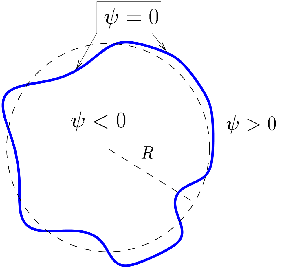
FIG. 1.:

FIG. 2.:

FIG. 3.:

FIG. 4.:

FIG. 5.:

REFERENCES

- [1] R. G. Cox, J. Fluid Mech. 37, 601 (1969).
- [2] D. Barthès-Biesel, J. Fluid Mech. 100, 831 (1980).
- [3] Y. Navot, Phys. of fluids 11, 990 (1999).
- [4] H. J. Deuling and W. Helfrich, J. Physique 37, 1335 (1976).
- [5] V. Lisy, B. Brutovsky, and A. V. Zatovsky, Phys. Rev. E 58, 7598 (1998).
- [6] S. F. Edwards and M. Schwartz, Physica A 167, 595 (1990).
- [7] M. Schwartz and S. F. Edwards, Physica A 153, 355 (1988).
- [8] Hu Gang, A. H. Krall, and D. A. Weitz, Phys. Rev. E 52, 6289 (1995).
- [9] S. T. Milner and S. A. Safran, Phys. Rev. A 36, 4371 (1987).
- [10] G. Dörries and G. Foltin, Phys. Rev. E 53, 2547 (1996).
- [11] Physica A 219, 253 (1995). K. Seki and S. Komura,
- [12] D. Bohm, Quantum Theory, Prentice-Hall (1951).
- [13] R. H. Landau, Quantum Mechanics II, Wiley-Interscience Publication, 2nd Ed. (1996).
- [14] G. Frenkel and M. Schwartz, Europhys. lett. 50, 628 (2000).
- [15] M. Schwartz and R. Brustein, J. Stat. Phys. 51, 585 (1988).
- [16] S. F. Edwards and M. Schwartz, Physica A 178, 236 (1991).
- [17] M. Doi and S. F. Edwards, The Theory of Polymer Dynamics, Oxford Science Publications (1986).