Geometry-dependent electrostatics near contact lines

Abstract

Long-ranged electrostatic interactions in electrolytes modify their contact angles on charged substrates in a scale and geometry dependent manner. For angles measured at scales smaller than the typical Debye screening length, the wetting geometry near the contact line must be explicitly considered. Using variational and asymptotic methods, we derive new transcendental equations for the contact angle that depend on the electrostatic potential only at the three phase contact line. Analytic expressions are found in certain limits and compared with predictions for contact angles measured with lower resolution. An estimate for electrostatic contributions to line tension is also given.

Modern microfluidic and patterning applications call for directed fluid flow and wetting on treated surfaces often exhibiting complex surface chemistry CHA95 ; PET92 ; TROIAN ; NAPL . Mechanisms of differential wetting of small droplets of electrolytes have also been exploited as electrically activated switches and micropumps CJKIM . In such systems, the effects of surface ionization have been found to be important CHA95 ; NAPL ; KAYSER ; DIGILOV ; FOKKINK .

Consequently, one often considers two immiscible fluids of dielectric constants $\epsilon_{0},\epsilon_{1}$ that partially wets an ionizable, rigid substrate, as shown in Figs. 1. The two liquids, depending on their individual pKa’s, will differentially hydrolyze/ionize substrates such as glass. Ionizable surfactants may also be adsorbed, imparting a fixed, relatively uniform surface charge $\sigma$ at the interfaces. Microscopically, surface tensions $\gamma$ arise from mismatches in short-ranged molecular interactions (e.g. van der Waal’s) among the various species. Electrostatic double layers also contribute to surface energies. The application of the classical Young-Dupré (Y-D) equation YDREF , $\gamma_{01}^{\prime}\cos\alpha^{*}\approx\gamma_{0s}^{\prime}-\gamma_{1s}^{\prime}$, with electrostatically modified surface energies (e.g. $\gamma_{1s}^{\prime}=\gamma_{1s}+{1\over 2}\sigma_{1}\varphi_{1}$, where $\sigma_{1}$ and $\varphi_{1}$, are surface charges and potentials in, say, liquid 1 far from the contact point $P$) is accurate provided the apparent contact angle $\alpha^{*}$ is measured at a point $P^{*}$ outside the range $\kappa^{-1}$ of the electric double layers. However, the screening length $\kappa^{-1}$, although typically smaller than the resolution of optical goniometry measurements, can be within the resolution (nanometers) of emerging angle measurement techniques using AFM POMPE . Even at lower resolutions, finite-sized double-layer effects may be relevant for contact angle measurements. For example, hydrolysis of pure water gives $\kappa^{-1}\sim 1\mu$m, while in organic mixtures, with fewer mobile ions, the screening length can be even longer NAPL . If the contact angle is measured at $P$, within the ionic double layers, the simple Y-D equation is not appropriate.

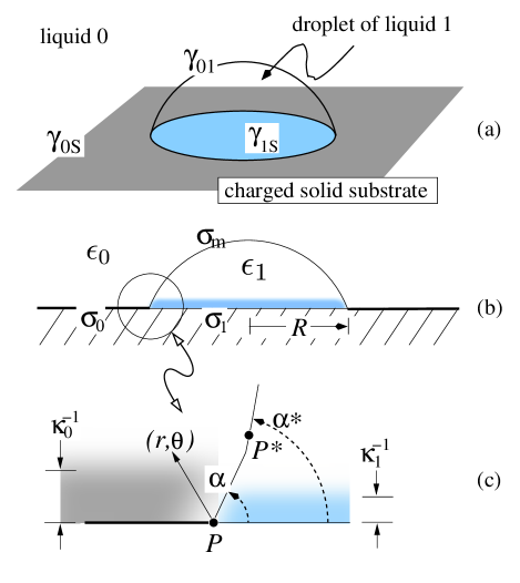
Figure 1: (a) Two liquids with dielectric constants $\epsilon_{0},\epsilon_{1}$ wets a charged substrate. (b) The substrate is ionized and acquires fixed charge densities of $\sigma_{0},\sigma_{1}$. Charged surfactants can also impart a surface charge $\sigma_{m}$ at the fluid-fluid interface. (c) In order to satisfy boundary conditions, the different screening layers deform near the contact point $P$.

Previous theories that consider surface energy modifications CHA95 ; KAYSER ; DIGILOV ; FOKKINK ; BUTKUS ; WHITE ; JPH , have either assumed microscopic-ranged interactions or infinite-system surface free energy changes (i.e. $\gamma\rightarrow\gamma+{1\over 2}\sigma\varphi$). Effects of the wedge-like geometry on the intrinsic electrostatics near the contact line have not been considered. In this letter, we derive formulae for the angle at the true three phase contact line in the presence of long-ranged electrostatic interactions. Rich features arise in this most simple and classic problem when geometry is self-consistently incorporated. We propose using weak ionic solutions as a system with precisely controllable electrostatics for studying charge contributions to contact angle and line tension forces. Our results are summarized by Eqns. (3), (11), and (16).

The “mechanical” free energy of an axisymmetric liquid droplet of footprint radius $R$ (cf. Figs. 1a,b) in contact with a flat, solid substrate is $G_{mech}=(\gamma_{1s}-\gamma_{0s})\int d{\bf r}+\gamma_{01}\oint d{\bf S}_{01}+G_{body}$, where $\gamma$ are the surface tensions sans electrostatic interactions, $d{\bf r}$ is the in-plane surface element, ${\bf S}$ is the liquid-liquid surface element. The $G_{body}$ term may include gravitational energy, $(\rho_{1}-\rho_{0})g/2\int h^{2}(r)d{\bf r}$, and/or Lagrange multipliers to e.g. fix droplet volumes of incompressible liquids. The electrostatic free energy for a specified surface charge ensemble, written as a functional of the local electrostatic potential $\varphi$ is CHOU

$$\begin{array}[]{ll}\displaystyle G_{e\ell}=\oint\sigma({\bf S})\varphi({\bf S})d{\bf S}-\int d{\bf r}dz\left[{\epsilon({\bf r},z)\over 8\pi}|\nabla\varphi|^{2}+U[\varphi]\right]\end{array}$$ (1)

where $U[\varphi({\bf r})]\equiv\sum_{i}e\nu_{i}c_{i}^{\infty}(\exp(-\nu_{i}\varphi({\bf r}))-1)$ is a term summing the interactions among mobile charged species $i$, each with valency $\nu_{i}$ and bulk concentration $c_{i}^{\infty}$. We have expressed all energy and length quantities in terms of $k_{B}T$ and the Bjerrum length $\ell_{B}=e^{2}/k_{B}T$. Variation of $G_{e\ell}[\varphi({\bf r}),\nabla\varphi({\bf r});h({\bf r}),\nabla h({\bf r})]$ with respect to $\varphi({\bf r})$ for a fixed droplet height function $h({\bf r})$ yields the Poisson-Boltzmann equation with appropriate boundary conditions. Similarly, variation of $G_{T}=G_{mech}+G_{e\ell}$ with respect to the droplet height $h({\bf r})$ determines the complete shape of the electrolyte droplet via

$$\gamma_{01}\partial^{2}_{{\bf t}}h_{\perp}({\bf r})=\left[{\epsilon\over 8\pi}|\nabla\varphi|^{2}+U[\varphi]\right]^{0}_{1},$$ (2)

where $h_{\perp}$ is the deformation normal to the tangent ${\bf t}$ relative to a constant slope. Further minimizing the boundary terms in $G_{T}$ (which are independent of $U[\varphi]$) with respect to the position of the contact point, $\delta G_{T}(z=0)/\delta R=0$, yields

$$\gamma_{01}\cos\alpha=(\gamma_{0s}-\gamma_{1s})+(\sigma_{0}-\sigma_{1})\varphi(P;\alpha).$$ (3)

The first two terms arise from setting the variations in the boundary terms of $G_{mech}$ to zero and reproduces the Young-Dupré equation. The last term in (3) is a new generalization of the Y-D equation and arises from minimizing the boundary terms of $G_{e\ell}$. The additional term depends only on the jump in the solid surface charge and the electrostatic potential $\varphi(P)$ at the three phase contact line $P$. This potential is found by solving the Poisson-Boltzmann equation $\nabla^{2}\varphi({\bf r})=U^{\prime}[\varphi({\bf r})]$ in the appropriate geometry, subject to boundary conditions. Therefore, $\varphi(P)$ will depend parametrically on the droplet shape (and hence the contact angle $\alpha$) near $P$. Equation (3) is exact provided the electrostatic energy is given by $G_{e\ell}$, and gives an implicit formula for predicting the contact angle $\alpha$.

In the following, we compute $\varphi(P;\alpha)$ in the linearized limit $(U[\varphi]\approx\kappa^{2}\varphi^{2}/2)$, valid for $e\varphi({\bf r})/k_{B}T\ll 1$, by solving Kelvin’s (aka Debye-Hückel) equation in each of the two fluid domains depicted in Figs. 1:

$$\Delta\varphi_{j}=\kappa_{j}^{2}\varphi_{j}(r,\theta)\quad\mbox{in fluid}\,j=0,1.$$ (4)

The screening lengths $\kappa_{j}^{-1}\equiv\left({4\pi e\over\epsilon_{j}}\sum_{i}\nu_{i}^{2}c_{i}^{\infty}\right)^{-1/2}$ are assumed much smaller than the dimensions of the droplet. Furthermore, neglecting gravity, (2) shows that $h_{\perp}({\bf r})$ varies (relative to a perfect wedge) over a length scale $L_{h}\sim\sqrt{\gamma_{01}/(\kappa\varphi^{2}(P))}$. Provided $L_{h}\gg\kappa^{-1}$, the wedge is distorted only in the region where $\varphi\approx 0$, sufficiently beyond the contact point $P$ to be appreciably influenced by electrostatic interactions. Thus, $\varphi(P)$ will be computed using a perfect wedge geometry. The boundary conditions associated with (4) in 2D wedge domains are

$$\begin{array}[]{c}\displaystyle\epsilon_{1}\partial_{\theta}\varphi_{1}(r,0)=4\pi r\sigma_{1}\\ \displaystyle\epsilon_{0}\partial_{\theta}\varphi_{0}(r,\pi)=-4\pi r\sigma_{0}\\ \displaystyle\varphi_{0}(r,\alpha)-\varphi_{1}(r,\alpha)=0\\ \displaystyle\epsilon_{0}\partial_{\theta}\varphi_{0}(r,\alpha)-\epsilon_{1}\partial_{\theta}\varphi_{1}(r,\alpha)=4\pi r\sigma_{m}.\end{array}$$ (5)

The linear problem defined above is related to the classic problem of wave scattering from a wedge, which remains a substantial mathematical and computational challenge RAWLINS . The problem is best attacked using the Lebedev-Kantorovich (LK) integral transform

$$f_{j}(x,\theta)=\int_{0}^{\infty}\varphi_{j}(r,\theta)K_{ix}(\kappa_{j}r){dr\over r}\equiv{\cal L}_{\kappa_{j}}\varphi_{j},$$ (6)

and its inverse

$$\varphi_{j}(r,\theta)={2\over\pi^{2}}\int_{0}^{\infty}f(x,\theta)K_{ix}(\kappa_{j}r)x\mbox{sh}(\pi x)dx\equiv{\cal L}^{-1}_{\kappa_{j}}f_{j}.$$ (7)

If the contact angle can be measured sufficiently close the contact point (closer than $\kappa_{j}^{-1}$, such as in POMPE ), the potential $\varphi(\kappa r\rightarrow P)$ can be easily expressed in terms of its transform $f(x,\theta)$. We will henceforth scale distance as $\xi=\kappa_{0}r$ and reinsert $\kappa_{0}$ back into the final, quoted results. Asymptotic analysis of the integral representation $K_{ix}(\xi)=(1/2)\int_{-\infty}^{\infty}\exp\left[-\xi\mbox{ch}t+ixt\right]dt$ yields $\lim_{\xi\rightarrow 0}K_{ix}(\xi)\sim(\sin xt^{*})/x$, where $t^{*}=\lim_{\xi\rightarrow 0}\cosh^{-1}(1/\xi)=\infty$. The limit $\lim_{t^{*}\rightarrow\infty}(\sin xt^{*})/x=\pi\delta(x)$, implies

$$\lim_{\xi\rightarrow 0}\varphi(\xi,\theta)=\lim_{x\rightarrow 0}\left[x^{2}f(x,\theta)\right].$$ (8)

We find analytic expressions for $\varphi(r,\theta)$ in two limiting cases that illustrate the full range of behaviors: $\kappa_{0}\approx\kappa_{1}$, and $\kappa_{1}\gg\kappa_{0}$. In the former case of nearly identical screening lengths unequal dielectric constants $\epsilon_{0}\neq\epsilon_{1}$ provide an nontrivial electric field jump across $\theta=\alpha$. In the latter case, we will choose a small screening length (e.g., high salt) in region 1 without loss of generality. In both cases, the potential can be expanded in the power series $\varphi_{j}(r,\theta)=\sum_{n=0}^{\infty}\mu^{(n)}(\varepsilon)\varphi_{j}^{(n)}(r,\theta)$, where $\varepsilon$ is a small parameter that depends on the ratio of screening lengths and the relevant regime:

$\kappa_{1}\approx\kappa_{0}$ limit - In this limit, $\mu^{(n)}(\varepsilon)=\varepsilon^{n}$ and $\varepsilon\equiv(\kappa_{1}/\kappa_{0})^{2}-1$. At each order $\varepsilon^{n}$ the governing equations are $\Delta\varphi_{0}^{(n)}=\varphi_{0}^{(n)}$ for $\theta\geq\alpha$, and $\Delta\varphi_{1}^{(n)}=\varphi_{1}^{(n)}+\varphi_{1}^{(n-1)}$ for $\theta\leq\alpha$. Upon applying ${\cal L}_{1}$ to the $n^{th}$ order Debye-Hückel equations, $\partial_{\theta}^{2}f_{0}^{(n)}=x^{2}f_{0}^{(n)}(x,\theta)$ and $\partial_{\theta}^{2}f_{1}^{(n)}=x^{2}f_{1}^{(n)}(x,\theta)=g^{(n-1)}(x,\theta)$ where $g^{(n-1)}(x,\theta)\equiv{\cal L}_{1}\varphi^{(n-1)}r^{2}(1-\delta_{n,0})$.

Similarly, the transformed boundary conditions at each order become $\partial_{\theta}f_{0}^{(n)}(x,\theta=\pi)=(2\pi^{2}\sigma_{0}/\epsilon_{0})\mbox{sech}(\pi x/2)\delta_{n,0}$, $\partial_{\theta}f_{1}^{(n)}(x,\theta=0)=-(2\pi^{2}\sigma_{1}/\epsilon_{1})\mbox{sech}(\pi x/2)\delta_{n,0}$, and $\epsilon_{1}\partial_{\theta}f_{1}^{(n)}(x,\theta=\alpha)-\epsilon_{0}\partial_{\theta}f_{0}^{(n)}(x,\theta=\alpha)=2\pi^{2}\sigma_{m}\mbox{sech}(\pi x/2)\delta_{n,0}$. Since $f_{1}^{(0)}(x,\theta)$ obeys a homogeneous equation, it is determined explicitly. The equations for $f_{1}^{(n)}(x,\theta)$ can be solved with the appropriate Green function $G(x,\theta,\theta^{\prime})=-\mbox{ch}\,x\theta_{<}\mbox{ch}\,x(\theta_{>}-\alpha)/(x\mbox{sh}\,x\alpha),\partial_{\theta^{\prime}}G(x,\theta,\theta^{\prime}=0,\alpha)=0$, where $\theta_{<}(\theta^{\prime}_{>})$ is the smaller(larger) of $\theta,\theta^{\prime}$. We obtained, after some algebra, an integral equation for $f_{1}(x,\theta)$. The first iteration of this integral equation yields

$$\varepsilon f_{1}^{(1)}(x,\theta)=\varepsilon\int_{0}^{\infty}\!\!dx^{\prime}\int_{0}^{\alpha}d\theta^{\prime}\,H(\theta,\theta^{\prime};x,x^{\prime})f_{1}^{(0)}(x^{\prime},\theta^{\prime})$$ (9)

where

$$\begin{array}[]{l}\>\displaystyle H(\theta,\theta^{\prime};x,x^{\prime})\equiv\\[13.0pt] \displaystyle{(\epsilon_{1}/4)G(\theta,\theta^{\prime};x)(x^{2}-x^{\prime 2})x^{\prime}\mbox{sh}\pi x^{\prime}\mbox{sh}x\alpha\over\left(\epsilon_{1}\mbox{sh}x\alpha+\epsilon_{0}\mbox{ch}x\theta\,\mbox{th}x(\pi-\alpha)\right)\mbox{sh}{\pi\over 2}(x+x^{\prime})\mbox{sh}{\pi\over 2}(x-x^{\prime})}.\end{array}$$ (10)

Upon integrating (9) over $\theta^{\prime}$, and using $f_{1}(x,\theta)\approx f_{1}^{(0)}(x,\theta)+\varepsilon f_{1}^{(1)}(x,\theta)$ in (8), we find $\varphi(P;\alpha)$ up to $O(\varepsilon)$:

$$\begin{array}[]{l}\displaystyle\varphi(P;\alpha)\sim{2\pi^{2}/\kappa_{0}\over\epsilon_{1}\alpha+\epsilon_{0}(\pi-\alpha)}\bigg{[}(\sigma_{0}+\sigma_{1}+\sigma_{m})\\[13.0pt] \>\hskip 8.53581pt+\varepsilon\big{(}\sigma_{0}S_{0}(\alpha;\lambda)+\sigma_{1}S_{1}(\alpha;\lambda)+\sigma_{m}S_{m}(\alpha;\lambda)\big{)}+O(\varepsilon^{2})\bigg{]}.\end{array}$$ (11)

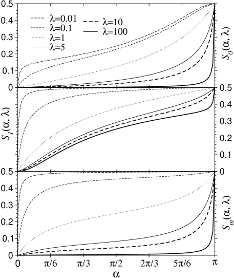
The first (zeroth order) term arises from $\lim_{x\rightarrow 0}x^{2}f_{1}^{(0)}$, while the $O(\varepsilon)$ terms can be expressed as single $\alpha$-dependent integrals $S_{i}(\alpha;\lambda)$. The functions $S_{i}$ are plotted vs. $\alpha$ in Fig. 2 for various dielectric mismatches $\epsilon_{0}/\epsilon_{1}\equiv\lambda$.

Figure 2: The functions $S_{i}(\alpha;\lambda=\epsilon_{0}/\epsilon_{1})$ representing the order $\varepsilon=\kappa_{1}^{2}/\kappa_{0}^{2}-1$ contributions to $\varphi(\alpha;P)$ (cf. Equation (11)).

The term that remains when $\kappa_{0}=\kappa_{1}$ and that multiplies all higher order terms in $\varepsilon$ is an effective angular average over the dielectrics $\epsilon_{0},\epsilon_{1}$. This dominant term is qualitatively different from that arising from simple surface tension renormalization $\gamma\rightarrow\gamma+{1\over 2}\sigma\varphi=\gamma+2\pi\sigma^{2}/(\epsilon\kappa)$. The higher order terms $S_{i}$ are determined with $\kappa_{1}$ relative to $\kappa_{0}$ and thus have their major effect when $\alpha\approx\pi$ as more of the volume is occupied by electrolyte of inverse screening length $\kappa_{1}$. For larger(smaller) $\lambda=\epsilon_{0}/\epsilon_{1}$, $S_{0}(S_{1})$ varies more significantly over a smaller range of angles $\alpha$, reflecting the importance of the charged surface on the lower dielectric slice. The effects of the liquid-liquid surface charge are symmetric with the interchange $\alpha\rightarrow\pi-\alpha$, $\epsilon_{0},\kappa_{0},\sigma_{0}\rightarrow\epsilon_{1},\kappa_{1},\sigma_{1}$ as expected.

$\kappa_{0}/\kappa_{1}\rightarrow 0$ limit - In the limit $\kappa_{1}\gg\kappa_{0}$ (4) become $\Delta\varphi_{0}=\varphi_{0}$ and $\Delta\varphi_{1}=\varepsilon^{-2}\varphi_{1}$, where $\varepsilon\equiv\kappa_{0}/\kappa_{1}$. Due to the strong screening in region 1, the potential under the surface wet by liquid 1 vanishes as $\sim\sigma_{1}(\epsilon_{1}\kappa_{1})^{-1}$. The first iteration makes the approximation $\varphi^{(0)}_{1}(r,\theta)=f_{1}^{(0)}\approx 0$. However, as a result of continuity of the potential at $\theta=\alpha$, and finite $\kappa_{0}$ and $\sigma_{0}$,

$$f_{0}^{(0)}(x,\theta)={2\pi^{2}\sigma_{0}\over\epsilon_{0}\kappa_{0}x}{\mbox{sh}x(\alpha-\theta)\over\mbox{ch}x(\pi-\alpha)\mbox{ch}(\pi x/2)}.$$ (12)

Thus, $\varphi_{0}(\theta>\alpha)={\cal L}_{1}^{-1}f_{0}^{(0)}\neq 0$. The first nonzero term in $\varphi(P)$ arises from using (12) in the jump condition at $\theta=\alpha$:

$$\begin{array}[]{l}\displaystyle\partial_{\theta}f_{1}(x,\alpha)-{\epsilon_{0}\over\epsilon_{1}}{\cal L}_{\varepsilon}{\cal L}^{-1}_{1}\partial_{\theta}f_{0}^{(0)}(x^{\prime},\alpha)=\varepsilon\left({2\pi^{2}\sigma_{m}\over\epsilon_{1}\kappa_{0}\mbox{ch}(\pi x/2)}\right).\end{array}$$ (13)

Upon expanding $K_{ix}(\xi)$ about its dominant contribution at small $\xi$ in the operator ${\cal L}^{-1}_{1}$ and performing the integration over $\xi$,

$$\begin{array}[]{l}\displaystyle{\cal L}_{\varepsilon}{\cal L}^{-1}_{1}\partial_{\theta}f_{0}^{(0)}(x^{\prime},\alpha)={\pi\sigma_{0}\over\epsilon_{0}\kappa_{0}}\sum_{n=0}^{\infty}{\varepsilon^{2n}\over n!}\times\\[13.0pt] \displaystyle\mbox{Im}\int_{0}^{\infty}{x^{\prime}\Gamma\left(n-{i\over 2}(x+x^{\prime})\right)\Gamma\left(n+{i\over 2}(x-x^{\prime})\right)e^{-ix^{\prime}\ln\varepsilon}\over\mbox{ch}(\pi x^{\prime}/2)\mbox{ch}x^{\prime}(\pi-\alpha)\Gamma(n+1-ix^{\prime})}dx^{\prime}\end{array}$$ (14)

The contour integral (14) can be performed exactly to find the two lowest order terms in $\varepsilon$ (for $n=0$, $\mu^{(1)}(\varepsilon)=\varepsilon^{\pi/(2\pi-2\alpha)}$ and $\mu^{(2)}(\varepsilon)=\varepsilon$) that must be considered. Using (8), our final result is

$$\varphi(P;\varepsilon/\alpha\rightarrow 0)\sim{2\pi^{2}\left(\sigma_{0}T_{0}(\alpha;\varepsilon)+\sigma_{m}\varepsilon\right)\over\alpha\epsilon_{1}\kappa_{0}}+O\left(\varepsilon^{{\pi\over\pi-\alpha}},\varepsilon^{2}\right),$$ (15)

where

$$T_{0}(\alpha;\varepsilon)\equiv{\pi\Gamma^{2}\left({\pi\over 4(\pi-\alpha)}\right)\varepsilon^{\pi/(2\pi-2\alpha)}\over 4(\pi-\alpha)^{2}\cos\left({\pi^{2}\over 4(\pi-\alpha)}\right)\Gamma\left({3\pi-2\alpha\over 2\pi-2\alpha}\right)}-{\varepsilon\over\cos\alpha}$$ (16)

is plotted in Fig. 3 for various values of $\varepsilon$.

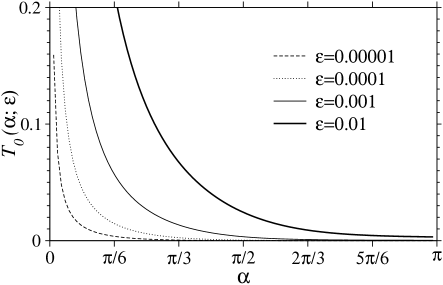
Figure 3: The function $T_{0}(\alpha;\varepsilon)$ (Eqn. (3)) that gives the $\sigma_{0}$-proportional term for the potential (Eqn. (15)) in the $\varepsilon=\kappa_{0}/\kappa_{1}\rightarrow 0$ limit.

The $\kappa_{0}/\kappa_{1}\rightarrow 0$ analysis fails for small $\alpha$, when the fully screened approximation breaks down as the interface approaches the $\sigma_{1}$-charged solid substrate. The correction to the potential is independent of $\sigma_{1}$ since it is screened out by a large $\kappa_{1}$. However, the jump condition across $\theta=\alpha$ preserves an $\epsilon_{1}$ dependence.

We have explicitly incorporated the geometric dependence of long-ranged electrostatic effects by deriving implicit equations for the contact angle valid for $R,L_{h}\sim(\epsilon/\sigma)\sqrt{\kappa\gamma_{01}}\gg\kappa^{-1}$. Our results show that for large mismatch in screening lengths, the potential at the contact point is proportional to the larger screening length $\kappa_{0}^{-1}$ but varies as an $\alpha$-dependent power of the mismatch $\kappa_{0}/\kappa_{1}$. In the $\kappa\approx\kappa_{1}$ case, the zeroth order contribution to the potential can yield a nonnegligible effect: For $\kappa\approx 50$nm, $\epsilon_{0}=20,\epsilon_{1}=80$, $\sigma_{0}-\sigma_{1}\approx 0.1$, $\sigma_{0},\sigma_{1}\sim O(1)$, the zeroth order correction to the surface energy varies from $\sim 1.5-0.4k_{B}T/\ell_{B}^{2}$ as $\alpha$ varies from $0$ to $\pi$. Since one $k_{B}T/\ell_{B}^{2}\simeq 8$ dyne/cm, the implicit $\alpha$ dependence should be observable as long as the contact angle can be measured at a distance within 50nm of $P$. Such measurements are possible using AFM techniques POMPE . Geometry-dependent electrostatics may also be an origin for the discrepancy between standard theory and measurements performed at low salt concentrations when screening length are long FOKKINK . Even when the apparent contact angle cannot be measured within a screening length of $P$, our results may provide a basis by which to better understand dynamic phenomena. Since contact line pinning can occur at a length scale smaller than $|P-P^{*}|$, the dynamics of the contact line may be better correlated with the true contact angle $\alpha$ rather than $\alpha^{*}$.

Note that $S_{i}(\alpha;\lambda)$ and $T_{0}(\alpha;\varepsilon)$, when used in (11) allow for the possibility of two solutions for $\alpha$. The physical value for $\alpha$ will be determined by the minimum energy solution that needs to be determined by the full solution of the shape along $P-P^{*}$. Therefore, in cases where two roots for $\alpha$ are possible, we expect the minimum energy solution to be the one closest to $\alpha^{*}$. Our results also imply that dramatic effects on wettability ($\alpha\approx 0,\pi$) can be induced by small changes in the physical parameters.

In our strictly 2D analyses, the only bounded solution when $\kappa_{0}=\sigma_{0}=0$ (e.g. air) is $\varphi(P;\alpha)=0$. However, an asymptotic analysis for the large radius ($R\gg L_{h},\kappa^{-1}$) limit is possible. The correction term to the Y-D equation resulting from such an analysis is proportional to $\tau\propto\sigma_{1}^{2}/(\kappa_{1}^{2}R)$ times an $\alpha$-dependent factor, and defines the line tension POMPE ; WHITE ; LAW99 arising from electrostatics. These electrostatic forces giving rise to line tension may be sufficiently long-ranged to be experimentally determined through a measurement of $\alpha$. Ionic strength may thus provide a controllable parameter with which to measure the elusive, and controversial, line tension of wetting LAW99 .

The author thanks G. Bal and J. B. Keller for discussions, and the NSF for support via grant DMS-9804370.

References

(1) R. C. Chatelier, C. J. Drummond, D. Y. C. Chan, Z. R. Vasić,
T. R. Gengenbach, and H. J. Griesser, Langmuir, 11(10), 4122, (1995).
(2) J. G. Petrov, A. Angelova, and D. Mobius,
Langmuir, 8(1), 206, (1992).
(3) A. A. Darhuber, S. M. Troian, S. M. Miller, and S. Wagner,
J. Appl. Phys.,87(11), 7768, (2000).
(4) F. T. Barranco, H. E. Dawson, J. M. Christener, and B. D. Honeyman,
Environ. Sci. Technol,31, 676,
(1997).
(5) M. G. Pollack, R. B. Fair, and A. D. Shenderov,
Appl. Phys. Lett.,77(11), 1725, (2000);
J. Lee, and C. J. Kim, J. Microelectromech. Systems,9(2), 171, (2000); H. J. J. Verheijen and M. W. J. Prins,
Langmuir,15,
6616, (1999).
(6) R. F. Kayser,
Phys. Rev. Lett.,56(17), 1831, (1986).
(7) R. Digilov, Langmuir,16, 6719,
(2000).
(8) L. G. J. Fokkink, and J. Ralston,
Colloids and Surfaces,36, 69, (1989).
(9) A. Adamson Physical Chemistry of Surfaces, (Wiley, 1973).
(10) T. Pompe and S. Herminghaus, Phys. Rev. Lett.,85, 1930,
(2000); F. Rieutord and M. Salmeron, J. Phys. Chem., B 102, 3941 (1998).
(11) M. A. Butkus, and D. Grasso, J. of Coll. and Int. Sci.,200,
172, (1998).
(12) Y. Solomentsev and L. R. White,
J. Coll. Int. Sci.,218, 122, (1999).
(13)Interfacial Forces and Fields, J.-P. Hsu, Ed.
Surfactant Science Series, 85 (Marcel Dekker, New York, 1999).
(14) K. A. Sharp and B. Honig, J. Phys. Chem.,94, 7684,
(1990); T. Chou, M. V. Jarić, and E. D. Siggia, Biophys. J., 72, 2042, (1997).
(15) A. D. Rawlins, Proc. R. Soc. Lond. A455, 2655, (1999).
(16) J. Y. Wang, S. Betelu, and B. M. Law, Phys. Rev. E, 63, (2001).