Measurement-induced Squeezing of a Bose-Einstein Condensate

Abstract

We discuss the dynamics of a Bose-Einstein condensate during its nondestructive imaging. A generalized Lindblad superoperator in the condensate master equation is used to include the effect of the measurement. A continuous imaging with a sufficiently high laser intensity progressively drives the quantum state of the condensate into number squeezed states. Observable consequences of such a measurement-induced squeezing are discussed.

Since its birth, quantum mechanics has led to an interpretational debate on the role played by the measurement process in its structure and its relationship to classical mechanics developed for macroscopic systems [1]. This debate has been enriched by the realization of new experimental techniques spanning from quantum jumps in single ion traps to macroscopic entangled states in various quantum systems. Recently, the production of atomic Bose-Einstein condensates of dilute atomic gases has also paved the way to the study of dynamical phenomena of macroscopic quantum systems with the precision characteristic of atomic physics [2].

Two optical techniques, absorption and dispersive imagings, have been used to monitor the dynamics of a Bose-Einstein condensate [2]. In the former the condensate interacts with a light beam resonant (or close to resonance) with an atomic transition. The output beam is attenuated proportionally to the column density of the condensate - the condensate density integrated along the line of sight of the imaging beam. The absorption of photons heats the condensate then strongly perturbing it, and in general a new replica of the condensate has to be produced to further study its dynamics. This measurement is, in the language of quantum measurement theory, of type-II since it destroys the state of the observed system and forbids the study of the dynamics of a single quantum system [3]. Repeated measurements on a Bose-Einstein condensate or, at the limit, its continuous monitoring are instead possible using its dispersive features, for instance through phase-contrast [4] or interference [5] imaging techniques. Off-resonance light is scattered by the condensate which induces phase-shifts thereby converted into light intensity modulations by homodyne or heterodyne detection. The off-resonant nature of the atom-photon interaction allows for a very low absorption rate and therefore low heating of the condensate. Thus, multiple shots of the same condensate can be taken - a type-I measurement - allowing to study with high accuracy several phenomena, like its formation in non-adiabatic conditions [6], short and long wavelength collective excitations [7], vortices and superfluid dynamics [8]. The effect of the measurement process is typically neglected in these analysis. A first attempt to include the measurement process in a two-mode configuration for the condensate has been discussed in [9]. Our main goal is to include the atom-photon interaction process present in dispersive imaging into the intrinsic dynamics of the condensate. We show that the measurement process induces number squeezing of the quantum state of the condensate, and we provide realistic estimates that suggest that the phenomenon could be observed with current experimental techniques.

Let us start the analysis with the effective interaction Hamiltonian between the off-resonant photons and the atoms, written as:

$$\hat{H}_{\rm int}={{\epsilon_{0}\chi_{0}}\over 2}\int d^{3}x~{}\hat{n}({\bf x}):{\bf E}^{2}:,$$ (1)

where $\hat{n}$ is the condensate density operator, and ${\bf E}$ the electric field due to the intensity $I$ of the incoming light. The coefficient $\chi_{0}$ represents the effective electric susceptibility of the atoms defined as $\chi_{0}=\lambda^{3}\delta/2\pi^{2}(1+\delta^{2})$, where we have introduced the light wavelength $\lambda$ and the light detuning measured in half-linewidths $\Gamma/2$ of the atomic transition, $\delta=(\omega-\omega_{\rm at})/(\Gamma/2)$. Equation (1) allows us to write the reduced master equation for the atomic degrees of freedom by a standard technique, i.e. by tracing out the photon degrees of freedom [10]. The photons are assumed to be in a plane-wave state with momentum along the impinging direction, corresponding to a wavevector ${\bf k}=k_{0}\hat{z}$ orthogonal to the imaging plane $x-y$. Unless tomographic techniques are used, the image results from a projection of the condensate onto the $x-y$ plane, by integrating along the $z$ direction. This demands to project the dynamics of the condensate into the imaging plane. In order to write a closed 2-D master equation to describe the $x-y$ dynamics we assume the condensate wavefunction to be factorizable as $\psi(x,y,z)=\phi(x,y)\Lambda(z)$. Such factorization holds if the confinement in the $z$-direction is strong enough to make the corresponding mean-field energy negligible with respect to the energy quanta of the confinement, i.e. $\hbar\omega_{z}>>Ng$, as recently demonstrated in [11], where $g=4\pi\hbar^{2}a/m$, with $a$ the s-wave scattering length, and $\omega_{z}$ the angular frequency of the confinement harmonic potential along the $z$ direction. The resulting reduced master equation in the imaging plane is written as [12]:

$${{d\hat{\rho}}\over dt} = -{i\over\hbar}[\hat{H}_{\rm{2D}},\hat{\rho}]$$ (3)

$$-\int d^{2}r_{1}\int d^{2}r_{2}K({\bf r}_{1}-{\bf r}_{2})[\hat{n}({\bf r}_{1}),[\hat{n}({\bf r}_{2}),\hat{\rho}]],$$

where $\hat{n}({\bf r})=\hat{\Psi}^{\dagger}\hat{\Psi}({\bf r})$ is the 2-D density operator. The effect of the measurement is taken into account through the second term in the right-hand side of Eq.(3). This equation preserves the total number of atoms, and corresponds to a quantum nondemolition [13] coupling between the atom and the optical fields [9, 14, 15, 16]. The measurement kernel $K$ has the expression:

$$K({\bf r})={{\pi\chi_{0}^{2}k_{0}I}\over 2\hbar c}\int d^{2}k\exp(-\xi^{2}k^{4}/4k_{0}^{2})\exp(i{\bf k}{\bf r}),$$ (4)

where $\xi$ is the lengthscale of the condensate in the $z$ direction, the width of the Gaussian state $\Lambda(z)$ under the abovementioned approximation. Equation (4) holds for a condensate having thickness in the $z$ direction $\xi\gg\lambda$. If the measurement kernel were a local one, $K({\bf r}_{1}-{\bf r}_{2})\simeq\delta({\bf r}_{1}-{\bf r}_{2})$, Eq.(3) would reduce to a Lindblad equation for the measurement of an infinite number of densities $\hat{n}({\bf r})$. This assumes that no spatial correlation is estabilished by the photon detection. However, the ultimate resolution limit in the imaging system depends on the photon wavelength, regardless of the pixel density of the detecting camera. The resolution lengthscale follows from Eq.(4) as a width of the kernel $\Delta r=(2\pi^{2}\xi/k_{0})^{1/2}=(\pi\xi\lambda)^{1/2}$, the geometrical average of the light wavelength and the condensate thickness $\xi$.

When the measurement outweighs the self dynamics, the wavefunction of the condensate is driven towards an eigenstate of the measurement apparatus. In that case the master equation (3) is solved by the eigenstates of the density operator $\hat{n}({\bf r})$, which are then pointer states [17], $\hat{\Psi}^{\dagger}({\bf r}_{1})\dots\hat{\Psi}^{\dagger}({\bf r}_{N})|0\rangle$. This state describes a “gas” of $N$ atoms localized at the points ${\bf r}_{1}\dots{\bf r}_{N}$. These states are manifestly not mean-field states so they cannot be described by any generalization of the Gross-Pitaevskii equation. A measurement strong in comparison to the Hamiltonian $\hat{H}_{\rm{2D}}$ will project an initial mean field condensate state onto one of the pointer states with a probability distribution for different ${\bf r}$’s given by the initial mean field wave function $p({\bf r})=\phi^{\star}\phi({\bf r})$. However, this dramatic change of the condensate state will not directly affect the condensate image since the homodyne current is given by the convolution $I({\bf r})\sim\int d^{2}r^{\prime}K({\bf r}-{\bf r}^{\prime})\langle\hat{n}({\bf r}^{\prime})\rangle$, which coarse-grains the density distribution over the resolution of the kernel $\Delta r^{2}$. The only effect on the image will be small statistical fluctuations: if the average number of atoms within a given resolution area of $\Delta r^{2}$ is $n$, then after the localization the number will be in the range $n\pm\sqrt{n}$.

When the system Hamiltonian $H_{\rm{2D}}$ is strong enough, it can change pointer states [18]. To quantify this phenomenon and the competition between localization induced by the measurement and the delocalization due to $\hat{H}_{\rm{2D}}$ we discretize Eq.(3) introducing a 2-D lattice with the natural choice for the lattice constant set by the resolution lengthscale $\Delta r$,

$${{d\hat{\rho}}\over dt}=-\frac{i}{\hbar}[-\hbar\omega\sum_{\langle k,l\rangle}\hat{\Psi}^{\dagger}_{k}\hat{\Psi}_{l}+\hat{V},\hat{\rho}\;]-S\sum_{l}[\hat{n}_{l},[\hat{n}_{l},\hat{\rho}]].$$ (5)

Here $\hat{\Psi}_{l}$ is an annihilation operator and $\hat{n}_{l}=\hat{\Psi}_{l}^{\dagger}\hat{\Psi}_{l}$ is the number operator at a lattice site $l$. The frequency of hopping between any nearest neighbor sites $\langle k,l\rangle$ is $\omega\approx\hbar/2m\Delta r^{2}$, which is $\hbar^{-1}$ times the characteristic kinetic energy. The potential energy operator is $\hat{V}=\sum_{l}U_{l}\hat{n}_{l}+G\hat{n}_{l}^{2}$, where $U_{l}$ is the trapping potential and $G=g/\xi\Delta r^{2}$. The effective measurement strength is $S\approx\int d^{2}rK({\bf r})/\Delta r^{2}=(2\pi/\Delta r)^{2}(\pi\chi_{0}^{2}k_{0}I/2\hbar c)$.

The Lindblad term in Eq. (5) is a sum of Lindblad terms for different lattice sites. Its pointer states are the Fock states $|\{N_{l}\}\rangle=|N_{1},N_{2},\ldots\rangle$ with definite occupation numbers $N_{l}$ at every site $l$. An initial pure mean-field state can be expanded in the Fock basis, $|\psi(0)\rangle=\sum_{\{N_{l}\}}\psi_{\{N_{l}\}}(0)|\{N_{l}\}\rangle$. If the initial mean-field wavefunction of the condensate is $\phi_{l}$, then the initial expectation value of the number of atoms at a site $l$ is $n_{l}(0)=N\phi^{\star}_{l}\phi_{l}$. Each site has a finite dispersion in the number of atoms, $\sigma_{l}(0)\simeq[n_{l}(0)]^{1/2}$. For large $n_{l}(0)$ the distribution of $N_{l}$ can be approximated by a Gaussian. If there were no self-Hamiltonian the Lindblad term would drive the state of the system into a mixed state of different Fock states $|\{N_{l}\}\rangle$. The mixed state describes an ensemble of outcomes of different realizations of the experiment. In a given realisation the outcome would be a definite Fock state $|\{N_{l}\}\rangle$ with random $N_{l}$ in the range $n_{l}(0)\pm\sigma_{l}(0)$. To describe a single realisation of the experiment we use a (Stratonovich) unraveling of the master equation by a stochastic Schrödinger equation (SSE) [19]

$$\frac{d}{dt}\psi_{\{N_{l}\}}=-\frac{i}{\hbar}\sum_{\{N^{\prime}_{l}\}}h_{\{N_{l},N^{\prime}_{l}\}}\psi_{\{N^{\prime}_{l}\}}-\frac{i}{\hbar}V_{\{N_{l}\}}\psi_{\{N_{l}\}}$$ (6)

$$+\psi_{\{N_{l}\}}\sum_{l}\left[-S(N_{l}-n_{l})^{2}+S\sigma_{l}^{2}+(N_{l}-n_{l})\theta_{l}\right]\;\;,$$ (7)

where the homodyne noises have averages $\overline{\theta_{l}(t)}=0$ and $\overline{\theta_{l_{1}}(t_{1})\theta_{l_{2}}(t_{2})}=2S\delta_{l_{1},l_{2}}\delta(t_{1}-t_{2})$. Here $n_{l}=\sum_{\{N_{l}\}}N_{l}|\psi_{\{N_{l}\}}|^{2}$, $\sigma_{l}=\sum_{\{N_{l}\}}(N_{l}-n_{l})^{2}|\psi_{\{N_{l}\}}|^{2}$, $h$ is the matrix element of the hopping Hamiltonian and $V_{\{N_{l}\}}=\sum_{l}(U_{l}N_{l}+GN_{l}^{2})$ is the potential energy. The unravelling does not change the pointer states [20].

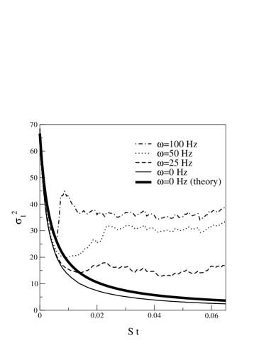
FIG. 1.: $\sigma_{1}^{2}(t)$ for a 1-D 3-mode configuration with $S=2\rm{s}^{-1}$, $n_{l}(0)=100$ and $\sigma_{l}^{2}(0)=66.6$. We show four single realizations of the experiment for different hopping frequencies. The thick solid line is the analytic solution $\sigma_{l}^{2}(t)=\sigma_{l}^{2}(0)/[1+4St\sigma_{1}^{2}(0)]$ for $\omega=0\;\rm{s}^{-1}$.

Equation (7) can be solved provided that we neglect the hopping term, $h=0$. In this case Fock states are fixed points because they are characterized by $N_{l}=n_{l}$ and $\sigma_{l}=0$. SSE is satisfied exactly by the ansatz

$$\psi_{\{N_{l}\}}(t)=e^{i\varphi_{\{N_{l}\}}}e^{-\frac{i}{\hbar}V_{\{N_{l}\}}t}\prod_{l}\frac{e^{-\frac{[N_{l}-n_{l}(t)]^{2}}{4\sigma_{l}^{2}(t)}}}{[2\pi\sigma_{l}^{2}(t)]^{1/4}},$$ (8)

when the parameters satisfy the equations of motion

$$\frac{d}{dt}\sigma_{l}^{2}=-4S\sigma_{l}^{4},\;\;\;\frac{d}{dt}n_{l}=2\sigma_{l}^{2}\theta_{l},$$ (9)

and $\varphi_{\{N_{l}\}}=\sum_{l}N_{l}{\rm Arg}(\phi_{l})$ are constant phases. The ansatz remains normalized as long as $\sigma_{l}^{2}\gg 1$ when summations over $N_{l}$ can be replaced by integrals. For an initial $\sigma_{l}^{2}(0)\simeq n_{l}(0)$ the dispersions shrink to zero (a Fock state) as $\sigma_{l}^{2}(t)=\sigma_{l}^{2}(0)/[1+4\sigma_{l}^{2}(0)St]$. Intuitively, the continuous reduction of number fluctuations is due to the weak nature of the measurement, and takes place on a time scale $\simeq 1/S\sigma^{2}_{l}(0)$. While $\sigma_{l}^{2}$’s shrink down to $\sigma_{l}^{2}\approx 1$ the means $n_{l}$ make random walks in the range $n_{l}(0)\pm\sigma_{l}(0)$. When $\sigma_{l}^{2}\ll 1$ our ansatz breaks down but the numerical simulations for 2- and 3-site models show that $n_{l}$ becomes frozen.

For non zero $h$, localization in a Fock state may be inhibited due to the hopping between nearest neighbor sites. Here a scaling argument is used to estimate the dependence on the physical parameters of $\sigma_{l}^{2}(\infty)$, the dispersion at which the measurement term and the hopping term in the SSE balance each other. We assume that the density distribution is smooth, i.e. any two nearest neighbor sites $k,l$ have close occupation numbers, $n_{k}\approx n_{l}$. For large occupation numbers, the element of the hopping Hamiltonian between $k$ and $l$ can be approximated by $\omega\sqrt{N_{k}N_{l}}\approx\omega\sqrt{n_{k}n_{l}}\approx\omega n_{l}$. The hopping mixes the amplitudes $\psi_{\{N_{l}\}}$ and $\psi_{\{N^{\prime}_{l}\}}$ which have negligibly close potential energies, $V_{\{N_{l}\}}\approx V_{\{N^{\prime}_{l}\}}$. We again assume that $\sigma_{l}^{2}\gg 1$ so that we can treat the occupation numbers $N_{l}$ as continuous variables. After neglecting the noise term, the SSE can be written as an eigenvalue ($\Omega$) problem

$$i\Omega\psi_{\{N_{l}\}}=\psi_{\{N_{l}\}}\sum_{l}\left[-S(N_{l}-n_{l})^{2}+S\sigma_{l}^{2}\right]$$ (10)

$$-i\omega\sum_{\langle k,l\rangle}\sqrt{n_{k}n_{l}}\left[\frac{\partial^{2}\psi_{\{N_{l}\}}}{\partial N_{k}^{2}}+\frac{\partial^{2}\psi_{\{N_{l}\}}}{\partial N_{l}^{2}}-2\frac{\partial^{2}\psi_{\{N_{l}\}}}{\partial N_{k}\partial N_{l}}\right]\;\;.$$ (11)

This equation is made parameter independent by rescaling $N_{l}\equiv\tilde{N}_{l}(\omega n_{l}/S)^{1/4}$ and $\Omega=\tilde{\Omega}\sum_{l}(S\omega n_{l})^{1/2}$, so the stationary solution of the rescaled equation must scale as $\sigma_{l}(\infty)\simeq(\omega n_{l}/S)^{1/4}$. In Figures 1 and 2 we show results of exact numerical simulations on a 1-D 3-site periodic lattice with 300 atoms which confirm the validity of these predictions. The solution without the hopping term, $\sigma^{2}_{l}(t)=\sigma_{l}^{2}(0)/[1+4St\sigma_{l}^{2}(0)]$, reaches its asymptotic value $\sigma_{l}(\infty)$ after a time $\tau_{l}\simeq[S\omega n_{l}(0)]^{-1/2}$.

We estimate the effect assuming the following parameters for the condensate and its imaging, relevant for the case of ${}^{87}{\rm Rb}$: $m=1.4\;10^{-25}{\rm kg}$, $a=5.8\rm{nm}$, $\lambda=780{\rm nm}$, $\chi_{0}=10^{-23}{\rm m}^{3}$, laser intensity $I=100{\rm mW}/{\rm cm}^{2}$, and a total number of atoms $N=10^{7}$. The width of the Gaussian $\Lambda(z)$ is assumed to be $\xi=10\mu{\rm m}$. The resolution of the kernel (4) is $\Delta r=(\pi\lambda\xi)^{1/2}=5\mu{\rm m}$. We also get $\omega=15\rm{s}^{-1}$, $S=65\rm{s}^{-1}$, and $G/\hbar=0.2\rm{s}^{-1}\ll S$. We assume that the initial condensate has a size of $(50\mu\rm{m})^{2}$ which implies $100$ occupied lattice sites with $n_{l}(0)\approx 10^{7}/100=10^{5}$ atoms per site and $\sigma_{l}(0)\simeq[n_{l}(0)]^{1/2}\approx 300$ atoms per site. Due to the measurement the dispersion shrinks $25$ times down to $\sigma_{l}(t=\infty)=(\omega n_{l}(0)/S)^{1/4}\approx 12$ atoms per site in a timescale $\tau_{l}=(S\omega n_{l}(0))^{-1/2}\approx 100\mu\rm{s}$. Until now we have neglected the off-resonance Rayleigh scattering due to the measurement. The same methods leading to Eqs.(3,4) also predict a Rayleigh depletion time of $\tau_{D}\approx 7\rm{ms}$, i.e. $70$ times longer than $\tau_{l}$ [12].

The dramatic $25$-fold shrinking of the dispersion in occupation number results in a quasi-Fock state. An exact Fock state would be $\hat{\Psi}^{\dagger}_{l_{1}}\dots\hat{\Psi}^{\dagger}_{l_{N}}|0\rangle$, where each atom can be assigned to exactly one lattice site and as such it is localized within the kernel resolution of $\Delta r^{2}$. The localization in an exact Fock state would cost a lot of kinetic energy. In our quasi-Fock state, as shown by the calculation of the expectation value of the hopping term in our ansatz state (8), as long as all $\sigma_{l}\gg 1$ the energy remains very close to the energy of the initial mean-field state.

A direct experimental test of our predictions and in particular of a simplified lattice model (5) can be made in the 1-D array of weakly linked mesoscopic traps of the experiment described in Ref.[21]. In this experiment the traps are created by a standing optical wave of wavelength $\lambda_{\rm st}=840{\rm nm}$ superimposed on a confining harmonic potential due to a magnetic trap. Given a transverse trapping angular frequency of $2\pi\times 120\rm{s}^{1}$ we estimate the transverse length of the condensates in each trap as the corresponding oscillator length, equal to $\xi=1\mu{\rm m}$. In the experiment each condensate has a $1/e$ width of $\Delta l=\lambda_{\rm st}/6$, therefore we estimate $G/\hbar=g/(2\hbar\Delta l(2\xi)^{2})\approx 40\rm{s}^{-1}$. Assuming one is in the range of parameters of the experiment for which the ground state of the condensate is close to a mean-field (quasi-coherent) state (for instance squeezing $s\simeq 3$ in Figure 2 of Ref.[21]), and that in each trap there are $n_{l}(0)\approx 100$ atoms of ${}^{87}{\rm Rb}$, the hopping frequency is $\omega=Gn_{l}(0)/\hbar s^{2}\approx 500\rm{s}^{-1}$.

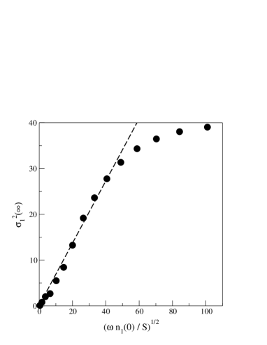
FIG. 2.: Asymptotic variance $\sigma_{1}^{2}(\infty)$ versus $(\omega n_{1}(0)/S)^{1/2}$ for a 1-D 3-mode configuration, with $S=2\rm{s}^{-1}$ and $n_{l}(0)=100$. The scaling $\sigma_{l}^{2}(\infty)\sim\omega^{1/2}$ applies for $(\omega n_{l}(0)/S)^{1/2}\ll\sigma_{l}^{2}(0)=67$ when $\omega\ll S\sigma^{4}_{l}(0)/n_{l}$. The straight line is a guide for the eye. In the opposite case $\sigma_{l}^{2}(\infty)$ does not increase above the dispersion of the initial mean-field state. The $\sigma_{l}^{2}(\infty)$ are averages over the noisy values at large $t$ of trajectories in Fig.1.

Suppose now that we add phase contrast imaging to the above experimental setup. The kernel resolution is $\Delta r=(\pi\xi\lambda)^{1/2}\approx 1.5\mu{\rm m}$, which implies there are 2 optical traps within the kernel resolution. The effective number of atoms within $\Delta r$ is therefore $n_{\rm pci}=200$, the effective self coupling is $G_{\rm pci}/\hbar=G/2\hbar=20\rm{s}^{-1}$ and the effective hopping frequency is $\omega_{\rm pci}=\omega/2=250\rm{s}^{-1}$. For a laser intensity of, say, $I=100{\rm mW}/{\rm cm}^{2}$, we obtain $S=500\rm{s}^{-1}$ and $\sigma_{l}(\infty)=3$ atoms per site after a localization time of $\tau_{l}=200\mu{\rm s}$ but much before a depletion time of $\tau_{D}=7\rm{ms}$. The final dispersion in the number of atoms per optical trap is $\sigma(\infty)=(\sigma_{l}(\infty)^{2}/2)^{1/2}=2$. The final squeezing factor will be $\sigma^{2}(0)/\sigma^{2}(\infty)\approx 50$, where we take $\sigma_{l}^{2}(0)=n_{l}(0)$. Such an enhancement of squeezing due to the measurement should be observable with the techniques of the experiment [21]

In conclusion, we have applied the theory of open quantum systems to include the back-action of a nondemolitive measurement into the dynamics of a Bose-Einstein condensate. We have shown that dispersive imaging with a sufficiently high laser intensity results in number squeezing of the condensate state. Our prediction can be tested in present-day experiments and could result in a significant improvement toward the implementation of Heisenberg-limited atom interferometry [22], and in a more general understanding of the back-action of other quantum-limited devices [13].

Acknowledgements. We thank L. Viola for useful discussions. D.A.R.D. and J.D. were supported in part by NSA.

REFERENCES

- [1] J. A. Wheeler and W. H. Zurek editors, Quantum Theory and Measurement (Princeton, NJ, Princeton University Press, 1983).
- [2] For a review see Bose-Einstein Condensation in Atomic Gases, Proceedings of the International School of Physics “Enrico Fermi”, edited by M. Inguscio, S. Stringari, and C. Wieman (IOS Press, Amsterdam, 1999).
- [3] W. Pauli, General Principles in Quantum Mechanics, Berlin, Springer, 1980 [Die allgemeinen Prinzipien der Wellenmechanik in Handbuch der Physik, Geiger and Schoel editors, XXIV, Berlin, Springer-Verlag, 1933].
- [4] M. R. Andrews, et al., Science 273, 84 (1996).
- [5] S. Kadlecek, J. Sebby, R. Newell, and T. G. Walker, Optics Lett. 26, 137 (2001).
- [6] H. J. Miesner, et al., Science 279, 1005 (1998).
- [7] M. R. Andrews, et al., Phys. Rev. Lett. 80, 2967 (1998); D. M. Stamper-Kurn, et al., Phys. Rev. Lett. 81, 500 (1998).
- [8] M. R. Matthews, et al., Phys. Rev. Lett. 83, 2498 (1999); R. Onofrio, et al., Phys. Rev. Lett. 85, 2228 (2000).
- [9] J. F. Corney and G. J. Milburn, Phys. Rev. A 58, 2399 (1998).
- [10] H. J. Carmichael, An Open Systems Approach to Quantum Optics (Springer, Berlin, 1993).
- [11] A. Görlitz, et al., Phys. Rev. Lett. 87, 130402 (2001).
- [12] D. A. R. Dalvit, J. Dziarmaga and R. Onofrio, in preparation.
- [13] V.B. Braginsky and F. Ya. Khalili, Quantum Measurements (Cambridge University Press, Cambridge, 1992).
- [14] R. Onofrio and L. Viola, Phys. Rev. A 58, 69 (1998).
- [15] C. F. Li and G. C. Huo, Phys. Lett. A 248, 117 (1998).
- [16] U. Leonhardt, T. Kiss, and P. Piwnicki, Eur. Phys. Journ. D 7, 413 (1999).
- [17] W. H. Zurek, Physics Today 44, 36 (1991).
- [18] W. H. Zurek, S. Habib and J. P. Paz, Phys. Rev. Lett.70, 1187 (1993).
- [19] D. Gatarek and N. Gisin, J. Math. Phys. 32, 2152 (1991).
- [20] D. A. R. Dalvit, J. Dziarmaga, and W.H. Zurek, Phys. Rev. Lett. 86, 373 (2001).
- [21] C.Orzel, et.al., Science 291, 2386 (2001).
- [22] P. Bouyer and M. A. Kasevich, Phys. Rev. A 56, R1083 (1997).