Microwave Conductivity due to Scattering from Extended Linear Defects
in $d$-Wave Superconductors

Abstract

Recent microwave conductivity measurements of detwinned, high-purity, slightly overdoped YBa₂Cu₃O_6.993 crystals reveal a linear temperature dependence and a near-Drude lineshape for temperatures between 1 and 20 K and frequencies ranging from 1 to 75 GHz. Prior theoretical work has shown that simple models of scattering by point defects (impurities) in $d$-wave superconductors are inconsistent with these results. It has therefore been suggested that scattering by extended defects such as twin boundary remnants, left over from the detwinning process, may also be important. We calculate the self-energy and microwave conductivity in the self-consistent Born approximation (including vertex corrections) for a $d$-wave superconductor in the presence of scattering from extended linear defects. We find that in the experimentally relevant limit ($\Omega,1/\tau\ll T\ll\Delta_{0}$), the resulting microwave conductivity has a linear temperature dependence and a near-Drude frequency dependence that agrees well with experiment.

]

I Introduction

Of the numerous phases of the high-$T_{c}$ cuprate phase diagram, the low temperature superconducting phase appears to be the least mysterious. All indications point to an order parameter of $d_{x^{2}-y^{2}}$ symmetry and well defined quasiparticle excitations above the condensate. [1, 2] An excellent probe of the low energy excitations of this $d$-wave superconductor is the measurement of low temperature microwave conductivity. Experimentally, the real part of the microwave conductivity, $\sigma(\Omega,T)$, can be extracted from microwave measurements of complex surface impedance $Z_{s}(\Omega,T)$. [3, 4, 5, 6, 7] Theoretically, at low temperatures, it is determined by calculating the linear response of a $d$-wave superconductor in the presence of scattering due to static disorder. [8, 9, 10, 11, 12, 13, 14, 15] (Low temperature is defined as low enough such that all inelastic scattering [16] is negligible.) The mystery is that, in this least mysterious of phases, the simplest theoretical models do not agree with experiment. [17]

The microwave conductivity of detwinned, high-purity, slightly overdoped YBa₂Cu₃O_6.993 was measured by Hosseini et al. [3] Data was taken at five frequencies between 1 and 75 GHz for temperatures from 1 to 95 K. Below 20 K, in the regime dominated by elastic scattering, they find that the microwave conductivity has an approximately linear temperature dependence and a near-Drude frequency dependence. Fitting the data to a Drude form, they extract a spectral weight that is linear in temperature (in agreement with the measured superfluid density) and an effective scattering rate, $1/\tau$, that is approximately constant over the entire low temperature regime (1 to 20 K).

From the extracted value of the scattering rate ($5.6\times 10^{10}\,\mbox{s}^{-1}$) and the frequency and temperature range of the experiments, it can be seen that these measurements correspond to the parameter regime $\Omega,1/\tau\ll T\ll\Delta_{0}$ where $\Delta_{0}$ is the gap maximum. For this parameter regime, the theoretical picture is as follows. A $d$-wave superconductor is characterized by an order parameter that vanishes linearly at each of four gap nodes. For $T\ll\Delta_{0}$, transport is dominated by low energy quasiparticle excitations generated in the vicinity of the nodes. For $1/\tau\ll T$, the quasiparticles are generated thermally, rather than by the presence of disorder. [18] (Hence, in what follows, we refer to this as the thermal regime.) The most straightforward model for such a system is one in which thermally generated nodal quasiparticles are scattered due to the presence of point defects such as impurities. Performing an impurity average and using a Kubo formula approach within the self-consistent $t$-matrix approximation, the self-energy and electrical conductivity have previously been calculated. [8, 9, 10, 17]

Surprisingly, the predictions of such calculations do not agree with the experimental results. The trouble comes in attempting to reproduce the constant scattering rate extracted from experiment. For a $d$-wave superconductor in the thermal regime, the anisotropic Dirac excitation spectrum yields a quasiparticle density of states that is linear in energy. This strong energy dependence of the density of states is then directly reflected in the results of the impurity $t$-matrix calculations. Such calculations yield $1/\tau\sim T$ and $\sigma\sim\mbox{const}$ in the Born limit and $1/\tau\sim 1/T$ and $\sigma\sim T^{2}$ in the unitary limit. More generally, over the full range of scattering strengths, it has been shown that simple models [19] of point defect (impurity) scattering are inconsistent with experiment. [17]

Despite this, we certainly expect the presence of impurities to make a significant contribution to the total scattering. However, the observed disagreement between theory and experiment suggests that an additional scattering mechanism may also be important. In what follows, we propose that this additional mechanism is scattering from extended linear defects. Our motivation for doing so is twofold. First of all, we note that scattering from a series of parallel lines differs from point defect scattering in an important way. While point defects scatter in all directions, line defects only scatter in the direction normal to their orientation. Hence, whereas point defect scattering samples the full quasiparticle density of states, line defect scattering restricts final states to those for which there is no change in the parallel component of momentum. Therefore, the line defect scattering rate need not inherit the strong energy dependence of the density of states and is thereby capable of exhibiting the less energy dependent form required to agree with experiment. Secondly, we note that upon growth, YBCO crystals are full of “lines”, twin boundary lines. Although the twin boundaries are subsequently removed via a detwinning procedure, remnants of their structure may be left behind in the form of extended linear defects. Since lines are prevalent in this material and line defects tend to exhibit features of the measured behavior, it is logical that we should examine the contribution made by line defect scattering. For simplicity, we consider herein a system where extended linear defects provide the sole scattering mechanism, leaving the analysis of a system with both line defects and point defects for future study.

In Sec. II, we discuss twinning in YBCO and the nature of the detwinning process. In light of the observed twinning structure and guided by the notion that the detwinning process leaves behind remnants in the form of line defects, we develop, in Sec. III, a model for quasiparticle scattering from extended linear defects in a $d$-wave superconductor. In Secs. IV and V, we calculate the resulting self-energy and microwave conductivity. For parameter values within the thermal regime, we obtain analytical results which are compared to experiment in Sec. VI A. Numerical results, including deviations from our analytical expressions and valid beyond the thermal regime, are presented in Sec. VI B. Conclusions are discussed in Sec. VII where we provide physical motivation for our calculated results and discuss the implications of our findings.

II Twin Boundaries in YBCO [20]

Twinning occurs naturally during the growth of oxygen deficient YBa₂Cu₃O_7-δ. At full oxygenation ($\delta=0$), the crystal structure is orthorhombic at room temperature with lattice parameters $a=3.227~{}\mbox{\AA}$ and $b=3.8872~{}\mbox{\AA}$, the latter being the orientation parallel to the CuO chain layer. [21] For nonzero $\delta$, oxygen vacancies are present in the CuO layer and the remaining oxygen can disorder onto sites perpendicular to the CuO chains, thereby reducing the orthorhombic distortion. [22] However, occupation of these off-chain sites is inhibited by repulsive interactions with oxygen located at on-chain sites. The formation of twin boundaries, which are abrupt boundaries between crystal domains with CuO chain orientations that differ by $90^{\circ}$, are the energetic compromise between decreasing the orthorhombicity and maintaining the CuO chain ordering.

The overdoped YBa₂Cu₃O_6.993 crystal studied by Hosseini et al. was prepared by annealing an as-grown crystal at $350^{\circ}$C for 50 days in flowing high purity oxygen. [3] Detwinning was accomplished by incrementally applying uniaxial stress in the $\widehat{ab}$ plane with the sample temperature fixed at $250^{\circ}$C in flowing high purity oxygen. Progress was monitored by viewing the sample through a microscope objective with a polarizer oriented at $45^{\circ}$ with respect to the crystalline axes. Domains with differing CuO chain orientations were then visible and the elimination of twin boundaries could be verified. The complete detwinning of a 1 mm² crystal can typically be accomplished within one day.

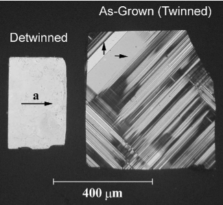
FIG. 1.: Photograph of as-grown (twinned) and detwinned single crystals of YBCO as viewed through an optical microscope under polarized light. In the as-grown sample, two different CuO chain orientations, visible as a difference in grayscale, are separated by twin boundaries oriented at $\pm 45^{\circ}$ to the horizontal. (Arrows highlight the two CuO chain orientations.) Darkened areas are regions of highly concentrated twin boundaries. In the detwinned sample, twin boundaries are no longer visible and the $\hat{a}$ axis is parallel to the horizontal throughout the crystal. (Photograph courtesy of R. Harris. [20])

An example of an as-grown twinned YBa₂Cu₃O_7-δ sample and a detwinned sample of YBa₂Cu₃O_6.993 are shown in Fig. 1. This picture was obtained by shining polarized white light onto the crystals at $45^{\circ}$ with respect to the crystalline axes and then observing through a polarizer oriented parallel to the incident light. In the as-grown sample, the two different CuO chain orientations are visible as a difference in grayscale. The lines oriented at $\pm 45^{\circ}$ which separate these regions are the twin boundaries. Darkened areas denote regions of highly concentrated twin boundaries. In the detwinned sample, there is a single orientation for all the CuO chains. Here, the $\hat{a}$ axis is parallel to the horizontal since this is the direction along which the uniaxial stress was applied. Note the absence of any visible twin boundaries in the detwinned crystal.

III Extended Linear Defect Scattering

Since line defect scattering has the appealing property that it does not sample the full quasiparticle density of states, we consider a model in which $d$-wave quasiparticles scatter from extended linear defects. In particular, we imagine that the line defects are arranged in a manner reflective of the twin boundary structure exhibited in YBCO prior to detwinning. That is, we consider domains of line defects within which the lines are parallel, oriented at either $+45^{\circ}$ or $-45^{\circ}$ to the crystal axes, and separated by distances on the order of microns. Our picture is that in the process of detwinning, neighboring twin boundaries are made to annihilate in order to eliminate regions in which the CuO chain orientation is disfavored by the applied uniaxial stress. Although this procedure is effective in removing the twin boundaries, it can leave behind defects along the lines at which the twin boundaries annihilate. While there may be multiple ways in which this can come to be, one example of a detwinning scenario through which line defects could be left behind is the following.

The twin boundaries in as-grown YBCO are $\pm 45^{\circ}$ lines which separate regions with horizontal CuO chains from regions with vertical CuO chains. Geometry dictates that the distance between oxygen sites on opposite sides of such a line is smaller than the normal oxygen-oxygen separation in the bulk. As a result, it is energetically advantageous for oxygen vacancies, which must be present in the CuO layer of doped YBCO, to be concentrated along twin boundary lines. Upon detwinning, a uniaxial stress is applied to favor one CuO chain orientation and force neighboring twin boundaries to approach each other and annihilate. As the twin boundaries move, the vacancies move with them until neighboring boundaries annihilate, leaving behind lines of oxygen vacancies. The resulting potential, felt by quasiparticles in the CuO₂ plane, is that of a collection of extended linear defects arranged in a pattern that reflects the original twinning structure. Note that this is just one example of a process that could yield line defects. As we shall see, however, our results will suggest that something similar to this is going on.

FIG. 2.: Schematic depiction of a single domain of extended linear defects. The line defects are aligned at $-45^{\circ}$ to the horizontal and spaced randomly in the $\hat{\bf r}_{\perp}$ direction with a 1d density $n_{T}$.

Consider a single domain in which all line defects are aligned at $-45^{\circ}$ to the horizontal axis. This situation is depicted schematically in Fig. 2. We denote the directions parallel and perpendicular to the defect lines as $\hat{\bf r}_{\parallel}$ and $\hat{\bf r}_{\perp}$ respectively. Now consider the effect of scattering off of such extended linear defects in 2d. Since all the lines are normal to the $r_{\perp}$ direction, they act as potential sources, $V(r_{\perp})$, that depend only on the $r_{\perp}$ coordinate. Fourier transforming, it is clear that such scattering events conserve the parallel component of momentum, $p_{\parallel}$, and are therefore one-dimensional in nature. Furthermore, since the distribution of line defects is random in the $r_{\perp}$ direction, this problem corresponds to an effective one-dimensional “impurity” problem (along $\hat{\bf r}_{\perp}$) in which $p_{\parallel}$ is conserved but not relevant to the scattering. Performing a 1d disorder average, properties of the resulting system can be calculated in terms of the 1d line defect density, $n_{T}$, and the 1d momentum-space line defect scattering potential, $V(p_{\perp}-k_{\perp})$.

FIG. 3.: Schematic depiction of the Brillouin zone of a $d$-wave superconductor in the presence of line defect scattering. The elliptical regions, labeled 1 through 4, denote (at a very exaggerated scale) four pockets of thermally generated nodal quasiparticles. In addition to the global momentum directions, $\hat{\bf p}_{\parallel}$ and $\hat{\bf k}_{\perp}$, defined parallel and perpendicular to the defect lines, we have also defined local momentum directions, $\hat{\bf k}_{1}$ and $\hat{\bf k}_{2}$, about each of the four nodes. The dashed lines denote scattering paths that conserve the parallel component of momentum.

Now consider the effect of this sort of one-dimensional scattering on the physics of a $d$-wave superconductor. We model a generic $d$-wave superconductor as a system with the Brillouin zone of a 2d square lattice and an order parameter of $d_{x^{2}-y^{2}}$ symmetry that vanishes at each of four nodal points on the Fermi surface. In the vicinity of each of these nodal points, the electronic dispersion, $\epsilon_{k}$, varies linearly across the Fermi surface and the order parameter, $\Delta_{k}$, varies linearly along the Fermi surface. As a result, near each of the gap nodes, the Bogoliubov quasiparticle excitation spectrum takes the anisotropic Dirac form $E_{k}=\sqrt{\epsilon_{k}^{2}+\Delta_{k}^{2}}=\sqrt{v_{f}^{2}k_{1}^{2}+v_{2}^{2}k_{2}^{2}}$ where the degree of anisotropy is expressed by the ratio of the Fermi velocity, $v_{f}$, to the gap velocity (slope), $v_{2}$, and the momenta, $k_{1}$ and $k_{2}$, are defined locally at each node such that in all cases, $\epsilon_{k}=v_{f}k_{1}$ and $\Delta_{k}=v_{2}k_{2}$. Hence, excitations are free at the nodal points and at temperatures much less than the gap maximum, quasiparticles are thermally generated within small regions about the gap nodes. The situation is depicted in Fig. 3 where the elliptical regions (labeled 1 through 4) denote four pockets of thermally generated quasiparticles. In the case of point defect (impurity) scattering, quasiparticles could be scattered either within the nodal pocket from which they originated (intra-node) or from one node to another (inter-node). [23] This is so because point defect scattering events do not conserve either component of momentum. However, due to the 1d nature of extended linear defect scattering, scattering events conserve the parallel component of momentum, $p_{\parallel}$. Therefore, in the presence of line defect scattering, quasiparticles can only be scattered along lines parallel to the $k_{\perp}$ axis in momentum space. Four such (dashed) lines are shown in Fig. 3. From the figure it is clear that the condition of $p_{\parallel}$ conservation means that we have two different kinds of nodes. For the odd nodes (1 and 3), quasiparticles can be scattered either intra-node ($1\rightarrow 1$ or $3\rightarrow 3$) or to their opposite-node ($1\rightarrow 3$ or $3\rightarrow 1$). Forbidden by $p_{\parallel}$ conservation is the adjacent-node scattering (i.e. $1\rightarrow 2$) that would be allowed for the point defect case. But for the even nodes (2 and 4), quasiparticles can only be scattered intra-node ($2\rightarrow 2$ or $4\rightarrow 4$). Here both adjacent-node and opposite-node scattering are forbidden by $p_{\parallel}$ conservation. Due to the clear difference between odd nodes and even nodes in the presence of line defect scattering, it will be important in the calculations that follow to always treat the odd node and even node cases separately. Furthermore, we should note that the designation of odd or even to a particular node is a direct result of our choice to consider a domain in which the line defects are aligned at $-45^{\circ}$ to the horizontal. To consider the other type of domain, where the line defects are aligned at $+45^{\circ}$ to the horizontal, we need only swap odd for even in all designations. With this model of thermally excited pockets of quasiparticles scattered by parallel randomly-spaced defect lines in mind, we proceed to calculate the resulting self-energy and microwave conductivity.

IV Self-Energy Calculation

For a superconductor at finite temperature, our calculations will employ Matsubara Green’s functions expressed in the $2\times 2$ matrix Nambu formalism. The bare Green’s function takes the form

$$\tilde{\cal{G}}_{0}({\bf k},i\omega)=\frac{1}{(i\omega)^{2}-E_{k}^{2}}\left(\begin{array}[]{cc}i\omega+\epsilon_{k}&\Delta_{k}\\ \Delta_{k}&i\omega-\epsilon_{k}\end{array}\right)$$ (1)

where the tilde denotes a Nambu-space matrix and $i\omega=i(2n+1)\pi k_{B}T$ is a fermionic Matsubara frequency. In the presence of scattering, the Green’s function is dressed via Dyson’s equation

$$\tilde{\cal{G}}({\bf k},i\omega)^{-1}=\tilde{\cal{G}}_{0}({\bf k},i\omega)^{-1}-\tilde{\Sigma}({\bf k},i\omega)$$ (2)

where

$$\tilde{\Sigma}({\bf k},i\omega)=\tilde{\Sigma}(k_{\perp},k_{\parallel},i\omega)=\left(\begin{array}[]{cc}\Sigma_{11}&\Sigma_{12}\\ \Sigma_{21}&\Sigma_{22}\end{array}\right)$$ (3)

is the Matsubara self-energy.

FIG. 4.: Self-energy within Born approximation.

In the Born approximation, this self-energy matrix can be calculated by evaluating the diagram in Fig. 4 to obtain

$$\tilde{\Sigma}(p_{\perp},p_{\parallel},i\omega)=n_{T}\sum_{k_{\perp}}\left|V(p_{\perp}-k_{\perp})\right|^{2}\tilde{\tau}_{3}\tilde{\cal{G}}(k_{\perp},p_{\parallel},i\omega)\tilde{\tau}_{3}$$ (4)

where $V(p_{\perp}-k_{\perp})$ is the line defect scattering potential, $n_{T}$ is the line defect density, and the $\tilde{\tau}_{i}$ are Pauli matrices in Nambu-space. Due to the 1d nature of the line defect scattering, $p_{\parallel}$ is conserved and we have integrated only over $k_{\perp}$. Since quasiparticles reside only in the vicinity of the four gap nodes, each momentum can be expressed by a node index, $j$, and a local momentum, $(k_{1},k_{2})$, defined about node $j$. Furthermore, it is useful to scale out the anisotropy of the excitation spectrum by defining local scaled momenta, $k^{\prime}_{1}\equiv v_{f}k_{1}$ and $k^{\prime}_{2}\equiv v_{2}k_{2}$, such that at each node $\epsilon_{k}=k^{\prime}_{1}$, $\Delta_{k}=k^{\prime}_{2}$, and $E_{k}=\sqrt{k^{\prime 2}_{1}+k^{\prime 2}_{2}}$. For convenience, we drop the primes in all that follows and take all locally defined momenta to be scaled momenta. Making use of these locally defined variables, we can replace

$$\sum_{k_{\perp}}\rightarrow\sum_{j}^{\prime}\int_{-\infty}^{\infty}\frac{dk}{2\pi v}$$ (5)

where the sum over node index $j$ is restricted to include only nodes that are crossed by the $k_{\perp}$ integration path, $k$ is the local scaled momentum component parallel to $k_{\perp}$ ($k_{1}$ or $k_{2}$), and $v$ is the corresponding velocity ($v_{f}$ or $v_{2}$). Similarly, we can replace the initial momentum, ($p_{\perp}$,$p_{\parallel}$), with an initial node index and an initial local scaled momentum, ($p_{1}$,$p_{2}$). As is clear from the dashed integration paths shown in Fig. 3, the details of these replacements depend on the type of node about which the quasiparticles reside prior to scattering. For quasiparticles initially near odd nodes (1 or 3), the node index sum yields both an intra-node scattering term and an opposite-node scattering term, in both of which $k_{1}$ is the local integration variable and $p_{2}$ is the local conserved variable. In contrast, for quasiparticles initially near even nodes (2 or 4), the node index sum yields only an intra-node scattering term, for which $k_{2}$ is the local integration variable and $p_{1}$ is the local conserved variable. It is therefore clear that once we change to local coordinates, we obtain from Eq. (4) two self-energy expressions, one for odd nodes and one for even nodes. For odd nodes:

$$\tilde{\Sigma}^{o}(p_{2},i\omega)=\frac{n_{T}}{2v_{f}}\tilde{\tau}_{3}\int\frac{dk_{1}}{\pi} \left[V_{1}^{2}\tilde{\cal{G}}^{o}(k_{1},p_{2},i\omega)\right.$$ (7)

$$\left.+V_{3}^{2}\tilde{\cal{G}}^{o}(k_{1},-p_{2},i\omega)\right]\tilde{\tau}_{3}$$

whereas for even nodes:

$$\tilde{\Sigma}^{e}(p_{1},i\omega)=\frac{n_{T}}{2v_{2}}\tilde{\tau}_{3}\int\frac{dk_{2}}{\pi}\left[V_{1}^{2}\tilde{\cal{G}}^{e}(p_{1},k_{2},i\omega)\right]\tilde{\tau}_{3}$$ (8)

where the superscripts ‘o’ and ‘e’ denote odd and even respectively. Here we have parameterized the scattering potential using the notation defined in Ref. [23] whereby $V_{1}$ defines the potential for an intra-node scattering event and $V_{3}$ defines the potential for an opposite-node scattering event. Note that for both odd nodes and even nodes, the self-energy is a function of frequency as well as the conserved component of the local scaled momentum, $p_{2}$ for the odd case and $p_{1}$ for the even case, but never the momentum component along $k_{\perp}$. This is a tremendous simplification since it means that the self-energy functions built into the right-hand side of Eqs. (7) and (8) will not be functions of the integration variables and can always be treated as constants with respect to the integrals. It is this fact that makes these equations tractable.

Since the bare Green’s function, Eq. (1), has no $\tilde{\tau}_{2}$ component, it is clear from the form of Eqs. (2) and (4) that it is self-consistent for the self-energy matrix to lack a $\tilde{\tau}_{2}$ component as well. It is therefore convenient to write the odd-node and even-node self-energy matrices in the form

$$\tilde{\Sigma}^{j}=\Sigma^{j}\tilde{\openone}+\Sigma_{1}^{j}\tilde{\tau}_{3}+\Sigma_{2}^{j}\tilde{\tau}_{1}$$ (9)

where $j=\{o,e\}$. It then follows from Eq. (2) that the corresponding dressed Green’s functions can be expressed as

$$\tilde{\cal{G}}^{j}(q_{1},q_{2},i\omega)=\frac{(i\omega-\Sigma^{j})\tilde{\openone}+(q_{1}+\Sigma_{1}^{j})\tilde{\tau}_{3}+(q_{2}+\Sigma_{2}^{j})\tilde{\tau}_{1}}{(i\omega-\Sigma^{j})^{2}-(q_{1}+\Sigma_{1}^{j})^{2}-(q_{2}+\Sigma_{2}^{j})^{2}}$$ (10)

where $(q_{1},q_{2})$ is the scaled momentum about a particular node and the self-energy components are functions of $q_{2}$ for odd nodes and $q_{1}$ for even nodes. This expression for the Green’s functions in terms of the self-energies together with Eqs. (7) and (8), giving the self-energies in terms of the Green’s functions, comprise matrix equations which can be solved self-consistently for the odd-node and even-node self-energies.

Let us consider the odd case first. Shifting the integration variable $k_{1}$ by $\Sigma^{o}_{1}$, we see that the $\tilde{\tau}_{3}$ term integrates to zero and therefore $\Sigma^{o}_{1}=0$. Then continuing $i\omega\rightarrow\omega+i\delta$ and making the ansatz (which will soon be shown valid) that $\Sigma^{o}$ is an even function of $p_{2}$ while $\Sigma^{o}_{2}$ is an odd function of $p_{2}$, we obtain

$$\Sigma^{o}=\int\frac{dk_{1}}{\pi}\frac{\alpha^{o}(\omega-\Sigma^{o})}{(\omega-\Sigma^{o})^{2}-(p_{2}+\Sigma^{o}_{2})^{2}-k_{1}^{2}}$$ (12)

$$\Sigma^{o}_{2}=\int\frac{dk_{1}}{\pi}\frac{-\alpha^{o}_{1}(p_{2}+\Sigma^{o}_{2})}{(\omega-\Sigma^{o})^{2}-(p_{2}+\Sigma^{o}_{2})^{2}-k_{1}^{2}}$$ (13)

$$\alpha^{o}\equiv\frac{n_{T}(V_{1}^{2}+V_{3}^{2})}{2v_{f}}\;\;\;\;\;\;\alpha^{o}_{1}\equiv\frac{n_{T}(V_{1}^{2}-V_{3}^{2})}{2v_{f}}$$ (14)

where $\Sigma^{o}=\Sigma^{o}(p_{2},\omega)$ and $\Sigma^{o}_{2}=\Sigma^{o}_{2}(p_{2},\omega)$ are now retarded functions.

For even nodes, we follow an analogous procedure and obtain results of the same form. This time, shifting the integration variable $k_{2}$ by $\Sigma^{e}_{2}$, it is the $\tilde{\tau}_{1}$ term that integrates to zero such that $\Sigma^{e}_{2}=0$. Continuing $i\omega\rightarrow\omega+i\delta$ to obtain retarded functions $\Sigma^{e}=\Sigma^{e}(p_{1},\omega)$ and $\Sigma^{e}_{1}=\Sigma^{e}_{1}(p_{1},\omega)$, we find

$$\Sigma^{e}=\int\frac{dk_{2}}{\pi}\frac{\alpha^{e}(\omega-\Sigma^{e})}{(\omega-\Sigma^{e})^{2}-(p_{1}+\Sigma^{e}_{1})^{2}-k_{2}^{2}}$$ (16)

$$\Sigma^{e}_{1}=\int\frac{dk_{2}}{\pi}\frac{\alpha^{e}_{1}(p_{1}+\Sigma^{e}_{1})}{(\omega-\Sigma^{e})^{2}-(p_{1}+\Sigma^{e}_{1})^{2}-k_{2}^{2}}$$ (17)

$$\alpha^{e}\equiv\alpha^{e}_{1}\equiv\frac{n_{T}V_{1}^{2}}{2v_{2}}$$ (18)

where we have defined $\alpha^{e}_{1}$ in analogy with the odd node case.

In light of the similarities between the odd and even results, we can treat both cases on the same footing by defining for $j=\{\mbox{odd},\mbox{even}\}$: $k=\{k_{1},k_{2}\}$, $p=\{p_{2},p_{1}\}$, $\Sigma=\{\Sigma^{o},\Sigma^{e}\}$, $\Sigma_{1}=\{\Sigma^{o}_{2},\Sigma^{e}_{1}\}$, $\alpha=\{\alpha^{o},\alpha^{e}\}$, $\alpha_{1}=\{\alpha^{o}_{1},\alpha^{e}_{1}\}$, and $\eta=\{-1,+1\}$. Hence, keeping in mind that our new variables have different meanings for odd and even nodes, we can write

$$\Sigma=\int\frac{dk}{\pi}\frac{\alpha(\omega-\Sigma)}{(\omega-\Sigma)^{2}-(p+\Sigma_{1})^{2}-k^{2}}$$ (20)

$$\Sigma_{1}=\int\frac{dk}{\pi}\frac{\eta\alpha_{1}(p+\Sigma_{1})}{(\omega-\Sigma)^{2}-(p+\Sigma_{1})^{2}-k^{2}}=\eta\frac{\alpha_{1}}{\alpha}\frac{p+\Sigma_{1}}{\omega-\Sigma}\Sigma$$ (21)

where the second equality in Eq. (21) was achieved by making use of Eq. (20). Solving Eq. (21) for $\Sigma_{1}$ in terms of $\Sigma$, plugging the result into Eq. (20), and evaluating the integral we find

$$\Sigma=\frac{-i\alpha}{\left[1-\left(\frac{p}{\omega-\gamma\Sigma}\right)^{2}\right]^{1/2}}\;\;\;\;\;\;\Sigma_{1}=\frac{(\gamma-1)p}{\omega-\gamma\Sigma}\Sigma$$ (22)

where we have defined $\gamma\equiv 1+\eta\alpha_{1}/\alpha$. This equation will be solved numerically in Sec. VI B to obtain an exact result for the self-energy.

Fortunately, in the experimentally relevant “thermal regime”, $\Omega,1/\tau\ll T\ll\Delta_{0}$, we can extract an approximate analytic result. As will be shown in the microwave conductivity calculation discussed in the following section, the energies of interest are $|\omega|$ on the order of $T$ and what we have called $\alpha$ is on the order of $1/\tau$. Thus, in the thermal regime, we are justified in taking the limit $|\omega|\gg\alpha$ such that we can set $\omega-\gamma\Sigma\approx\omega$. As a result, defining real and imaginary parts via $\Sigma=\Lambda-i\Gamma$ and $\Sigma_{1}=\Lambda_{1}-i\Gamma_{1}$, we find the approximate expressions

$$\Gamma\approx\alpha\frac{\theta(|\omega|-|p|)}{\sqrt{1-\left(\frac{p}{\omega}\right)^{2}}}\;\;\;\;\;\;\Lambda\approx-\alpha\,\mbox{sgn}(\omega)\frac{\theta(|p|-|\omega|)}{\sqrt{\left(\frac{p}{\omega}\right)^{2}-1}}$$ (24)

$$\Gamma_{1}\approx\eta\alpha_{1}\frac{p}{\omega}\frac{\theta(|\omega|-|p|)}{\sqrt{1-\left(\frac{p}{\omega}\right)^{2}}}\;\;\;\;\;\;\Lambda_{1}\approx-\eta\alpha_{1}\frac{p}{|\omega|}\frac{\theta(|p|-|\omega|)}{\sqrt{\left(\frac{p}{\omega}\right)^{2}-1}}$$ (25)

where the sharp cutoffs of the theta-functions are clearly artifacts of our approximation that are smoothed away in the exact solution. In the following section, we will make use of these thermal-regime self-energy functions to obtain an analytic expression for the microwave conductivity in the experimentally relevant parameter regime.

V Microwave Conductivity Calculation

The electrical conductivity tensor can be calculated by means of the Kubo formula

$$\tensor{\sigma}(\Omega,T)=-\frac{\mbox{Im}\,\tensor{\Pi}_{ret}(\Omega)}{\Omega}$$ (26)

where $\tensor{\Pi}_{ret}(\Omega)=\tensor{\Pi}(i\Omega\rightarrow\Omega+i\delta)$ and $\tensor{\Pi}(i\Omega)$ is the Matsubara polarization function (or current-current correlation function). Evaluating the diagram in Fig. 5(a) we find

FIG. 5.: Polarization bubble and dressed vertex within Born approximation.

$$\tensor{\Pi}(i\Omega) = \frac{1}{\beta}\sum_{i\omega}\sum_{p}e^{2}v_{f}^{2}\hat{\bf v}_{fp}$$ (27)

$$\times \mbox{Tr}\left[\tilde{\cal{G}}({\bf p},i\omega)\tilde{\cal{G}}({\bf p},i\omega+i\Omega)\tilde{\bf\Gamma}({\bf p},i\omega,i\Omega)\right]$$ (28)

where $\hat{\bf v}_{fp}$ points in the direction of the Fermi velocity and $\tilde{\bf\Gamma}$ is the dressed vertex function. Including vertex corrections within the Born approximation, $\tilde{\bf\Gamma}$ is calculated by evaluating the ladder diagrams in Fig. 5(b). Doing so, we obtain

$$\tilde{\bf\Gamma} (p_{\perp},p_{\parallel},i\omega,i\Omega)=\hat{\bf v}_{fp}\tilde{\openone}+\sum_{k_{\perp}}n_{T}\left|V(p_{\perp}-k_{\perp})\right|^{2}$$ (30)

$$\times\tilde{\tau}_{3}\tilde{\cal{G}}(k_{\perp},p_{\parallel},i\omega+i\Omega)\tilde{\bf\Gamma}(k_{\perp},p_{\parallel},i\omega,i\Omega)\tilde{\cal{G}}(k_{\perp},p_{\parallel},i\omega)\tilde{\tau}_{3}$$

where $n_{T}$ is the line defect density and $V(p_{\perp}-k_{\perp})$ is the line defect scattering potential. Once again, due to the 1d nature of our scattering, the momentum component parallel to the defect lines, $p_{\parallel}$, is conserved and we only integrate over the perpendicular component, $k_{\perp}$. Replacing momentum integrals by sums over node index and integrals over local scaled momenta, the polarization tensor takes the form

$$\tensor{\Pi} (i\Omega)=e^{2}v_{f}^{2}\sum_{j=1}^{4}\hat{\bf v}_{f}^{j}\hat{\bf v}_{f}^{j}\frac{1}{\beta}\sum_{i\omega}\int\frac{d^{2}p}{(2\pi)^{2}v_{f}v_{2}}$$ (33)

$$\times\mbox{Tr}\left[\tilde{\cal{G}}^{j}({\bf p},i\omega)\tilde{\cal{G}}^{j}({\bf p},i\omega+i\Omega)\left(\tilde{\openone}+\tilde{\Lambda}^{j}({\bf p},i\omega,i\Omega)\right)\right]$$

where we have defined a vertex correction function, $\tilde{\Lambda}^{j}$, such that

$$\tilde{\bf\Gamma}^{j}({\bf p},i\omega,i\Omega)=\hat{\bf v}_{f}^{j}\left(\tilde{\openone}+\tilde{\Lambda}^{j}({\bf p},i\omega,i\Omega)\right).$$ (35)

Note that $\tilde{\Lambda}^{j}$ depends only on the conserved component of the scaled local momentum (i.e. $\tilde{\Lambda}^{o}=\tilde{\Lambda}^{o}(p_{2},i\omega,i\Omega)$ while $\tilde{\Lambda}^{e}=\tilde{\Lambda}^{e}(p_{1},i\omega,i\Omega)$). Since quasiparticles in odd nodes (1 or 3) can be scattered either intra-node or to the opposite-node while quasiparticles in even nodes (2 or 4) can only be scattered intra-node, we must treat the odd and even cases separately as we proceed to calculate the vertex correction.

For odd nodes, Eqs. (LABEL:eq:vertex1) and (35) yield

$$\tilde{\Lambda}^{o}(p_{2}) = \frac{n_{T}V_{1}^{2}}{2v_{f}}\int\frac{dk_{1}}{\pi}\tilde{\tau}_{3}\tilde{\cal{G}}^{o}(k_{1},p_{2},i\omega+i\Omega)$$ (36)

$$\times \left(\tilde{\openone}+\tilde{\Lambda}^{o}(p_{2})\right)\tilde{\cal{G}}^{o}(k_{1},p_{2},i\omega)\tilde{\tau}_{3}$$ (37)

$$- \frac{n_{T}V_{3}^{2}}{2v_{f}}\int\frac{dk_{1}}{\pi}\tilde{\tau}_{3}\tilde{\cal{G}}^{o}(k_{1},-p_{2},i\omega+i\Omega)$$ (38)

$$\times \left(\tilde{\openone}+\tilde{\Lambda}^{o}(-p_{2})\right)\tilde{\cal{G}}^{o}(k_{1},-p_{2},i\omega)\tilde{\tau}_{3}$$ (39)

where we have suppressed the frequency dependence of $\tilde{\Lambda}^{o}$ for simplicity. Taking the Nambu-space trace, noting that $\tilde{\tau}_{3}\tilde{\cal{G}}^{o}(p_{2})\tilde{\tau}_{3}=\tilde{\cal{G}}^{o}(-p_{2})$, and using the cyclic properties of the trace, we find

$$\mbox{Tr}\left[\tilde{\Lambda}^{o}(p_{2})\right]=\mbox{Tr}\bigg{[} \frac{n_{T}}{2v_{f}}\tilde{I}^{o}(p_{2})\Big{(}(V_{1}^{2}-V_{3}^{2})\tilde{\openone}$$ (41)

$$+V_{1}^{2}\tilde{\Lambda}^{o}(p_{2})-V_{3}^{2}\tilde{\tau}_{3}\tilde{\Lambda}^{o}(-p_{2})\tilde{\tau}_{3}\Big{)}\bigg{]}$$

where we have defined

$$\tilde{I}^{o}(p_{2}) \equiv \int\frac{dk_{1}}{\pi}\tilde{\cal{G}}^{o}(k_{1},p_{2},i\omega)\tilde{\cal{G}}^{o}(k_{1},p_{2},i\omega+i\Omega)$$ (42)

$$\equiv I^{o}(p_{2})\tilde{\openone}+I_{1}^{o}(p_{2})\tilde{\tau}_{1}$$ (43)

with $I^{o}(p_{2})$ an even function and $I^{o}_{1}(p_{2})$ an odd function. Note that the fact that $\tilde{I}^{o}(p_{2})$ can be written in this form is merely assumed at this point but will be demonstrated later. Manipulating further and making the additional assumption (which will soon be shown valid) that $\mbox{Tr}[\tilde{\Lambda}^{o}(p_{2})]$ is an even function and $\mbox{Tr}[\tilde{\tau}_{1}\tilde{\Lambda}^{o}(p_{2})]$ is an odd function, we can write

$$\mbox{Tr}\left[\tilde{\Lambda}^{o}\right]=\alpha_{1}^{o}I^{o}\left(2+\mbox{Tr}\left[\tilde{\Lambda}^{o}\right]\right)+\alpha_{1}^{o}I^{o}_{1}\,\mbox{Tr}\left[\tilde{\tau}_{1}\tilde{\Lambda}^{o}\right]$$ (44)

where $\alpha_{1}^{o}=n_{T}(V_{1}^{2}-V_{3}^{2})/2v_{f}$, as defined in Eq. (14), and we have now suppressed the $p_{2}$ dependences. Going back to Eq. (39) but this time multiplying by $\tilde{\tau}_{1}$ before taking the trace, we can proceed along analogous lines to show that

$$\mbox{Tr}\left[\tilde{\tau}_{1}\tilde{\Lambda}^{o}\right]=\alpha_{1}^{o}J^{o}\,\mbox{Tr}\left[\tilde{\tau}_{1}\tilde{\Lambda}^{o}\right]+\alpha_{1}^{o}J^{o}_{1}\left(2+\mbox{Tr}\left[\tilde{\Lambda}^{o}\right]\right)$$ (45)

where we have now defined

$$\tilde{J}^{o}(p_{2}) \equiv -\int\frac{dk_{1}}{\pi}\tilde{\cal{G}}^{o}(k_{1},p_{2},i\omega)\tilde{\tau}_{1}\tilde{\cal{G}}^{o}(k_{1},p_{2},i\omega+i\Omega)$$ (46)

$$\equiv J^{o}_{1}(p_{2})\tilde{\openone}+J^{o}(p_{2})\tilde{\tau}_{1}$$ (47)

with $J^{o}(p_{2})$ an even function and $J^{o}_{1}(p_{2})$ an odd function. Solving Eqs. (44) and (45) simultaneously, we find that

$$\mbox{Tr}\left[\tilde{\Lambda}^{o}\right]=\frac{2\alpha_{1}^{o}\left(I^{o}+\frac{\alpha_{1}^{o}I^{o}_{1}J^{o}_{1}}{1-\alpha_{1}^{o}J^{o}}\right)}{1-\alpha_{1}^{o}\left(I^{o}+\frac{\alpha_{1}^{o}I^{o}_{1}J^{o}_{1}}{1-\alpha_{1}^{o}J^{o}}\right)}$$ (48)

and

$$\mbox{Tr}\left[\tilde{\tau}_{1}\tilde{\Lambda}^{o}\right]=\frac{\frac{2\alpha_{1}^{o}J^{o}_{1}}{1-\alpha_{1}^{o}J^{o}}}{1-\alpha_{1}^{o}\left(I^{o}+\frac{\alpha_{1}^{o}I^{o}_{1}J^{o}_{1}}{1-\alpha_{1}^{o}J^{o}}\right)}$$ (49)

from which it is clear, given the defined parity of $I^{o}$, $I^{o}_{1}$, $J^{o}$, and $J^{o}_{1}$, that as a function of $p_{2}$, $\mbox{Tr}[\tilde{\Lambda}^{o}]$ is odd and $\mbox{Tr}[\tilde{\tau}_{1}\tilde{\Lambda}^{o}]$ is even, in agreement our prior assumptions. Finally, using Eqs. (43) and (44) and the fact that the Pauli matrices are traceless, we can write

$$\mbox{Tr}\left[\tilde{\Lambda}^{o}(p_{2})\right]=\alpha_{1}^{o}\,\mbox{Tr}\left[\tilde{I}^{o}(p_{2})\left(\tilde{\openone}+\tilde{\Lambda}^{o}(p_{2})\right)\right]$$ (50)

which will prove a useful expression in what follows.

For even nodes, the vertex correction function takes the form

$$\tilde{\Lambda}^{e}(p_{1}) = \frac{n_{T}V_{1}^{2}}{2v_{2}}\int\frac{dk_{2}}{\pi}\tilde{\tau}_{3}\tilde{\cal{G}}^{e}(p_{1},k_{2},i\omega+i\Omega)$$ (51)

$$\times \left(\tilde{\openone}+\tilde{\Lambda}^{e}(p_{1})\right)\tilde{\cal{G}}^{e}(p_{1},k_{2},i\omega)\tilde{\tau}_{3}.$$ (52)

Note that this even-node expression is of the same form as the corresponding odd-node expression, Eq. (39), but is somewhat simpler since we need only consider intra-node scattering. Taking the trace and cyclically permuting within the trace, we find

$$\mbox{Tr}\left[\tilde{\Lambda}^{e}(p_{1})\right]=\alpha_{1}^{e}\,\mbox{Tr}\left[\tilde{I}^{e}(p_{1})\left(\tilde{\openone}+\tilde{\Lambda}^{e}(p_{1})\right)\right]$$ (54)

where $\alpha_{1}^{e}=n_{T}V_{1}^{2}/2v_{f}$, as defined in Eq. (18), and we have defined

$$\tilde{I}^{e}(p_{1}) \equiv \int\frac{dk_{2}}{\pi}\tilde{\cal{G}}^{e}(p_{1},k_{2},i\omega)\tilde{\cal{G}}^{e}(p_{1},k_{2},i\omega+i\Omega)$$ (55)

$$\equiv I^{e}(p_{1})\tilde{\openone}+I_{1}^{e}(p_{1})\tilde{\tau}_{3}.$$ (56)

Making use of the second equality in Eq. (56) and further defining

$$\tilde{J}^{e}(p_{1}) \equiv \int\frac{dk_{2}}{\pi}\tilde{\cal{G}}^{e}(p_{1},k_{2},i\omega)\tilde{\tau}_{3}\tilde{\cal{G}}^{e}(p_{1},k_{2},i\omega+i\Omega)$$ (57)

$$\equiv J^{e}_{1}(p_{1})\tilde{\openone}+J^{e}(p_{1})\tilde{\tau}_{3}$$ (58)

we obtain two coupled equations for $\mbox{Tr}[\tilde{\Lambda}^{e}]$ and $\mbox{Tr}[\tilde{\tau}_{3}\tilde{\Lambda}^{e}]$,

$$\mbox{Tr}\left[\tilde{\Lambda}^{e}\right]=\alpha_{1}^{e}I^{e}\left(2+\mbox{Tr}\left[\tilde{\Lambda}^{e}\right]\right)+\alpha_{1}^{e}I^{e}_{1}\,\mbox{Tr}\left[\tilde{\tau}_{3}\tilde{\Lambda}^{e}\right]$$ (59)

$$\mbox{Tr}\left[\tilde{\tau}_{3}\tilde{\Lambda}^{e}\right]=\alpha_{1}^{e}J^{e}\,\mbox{Tr}\left[\tilde{\tau}_{3}\tilde{\Lambda}^{e}\right]+\alpha_{1}^{e}J^{e}_{1}\left(2+\mbox{Tr}\left[\tilde{\Lambda}^{e}\right]\right).$$ (60)

Solving simultaneously yields

$$\mbox{Tr}\left[\tilde{\Lambda}^{e}\right]=\frac{2\alpha_{1}^{e}\left(I^{e}+\frac{\alpha_{1}^{e}I^{e}_{1}J^{e}_{1}}{1-\alpha_{1}^{e}J^{e}}\right)}{1-\alpha_{1}^{e}\left(I^{e}+\frac{\alpha_{1}^{e}I^{e}_{1}J^{e}_{1}}{1-\alpha_{1}^{e}J^{e}}\right)}$$ (61)

which has precisely the same form as in the odd case.

Due to this similarity in form, we can unite the odd and even cases by using the superscript $j=\{o,e\}$ and defining a generalized integration variable $k=\{k_{1},k_{2}\}$ and a generalized conserved variable $p=\{p_{2},p_{1}\}$. Doing so, we can define

$$K^{j}(p,i\omega,i\Omega) \equiv \frac{1}{2\alpha_{1}^{j}}\mbox{Tr}\left[\tilde{\Lambda}^{j}(p,i\omega,i\Omega)\right]$$ (62)

$$= \frac{I^{j}+\frac{\alpha_{1}^{j}I^{j}_{1}J^{j}_{1}}{1-\alpha_{1}^{j}J^{j}}}{1-\alpha_{1}^{j}\left(I^{j}+\frac{\alpha_{1}^{j}I^{j}_{1}J^{j}_{1}}{1-\alpha_{1}^{j}J^{j}}\right)}$$ (63)

and note via Eqs. (50) and (54) that

$$\mbox{Tr}\left[\tilde{I}^{j}(p,i\omega,i\Omega)\left(\tilde{\openone}+\tilde{\Lambda}^{j}(p,i\omega,i\Omega)\right)\right]=2K^{j}(p,i\omega,i\Omega).$$ (64)

Then going back to our expression for the polarization tensor, Eq. (LABEL:eq:bub2), and noting that

$$\hat{\bf v}_{f}^{1}\hat{\bf v}_{f}^{1}+\hat{\bf v}_{f}^{3}\hat{\bf v}_{f}^{3} = \tensor{\openone}+\tensor{\tau}_{1}$$ (65)

$$\hat{\bf v}_{f}^{2}\hat{\bf v}_{f}^{2}+\hat{\bf v}_{f}^{4}\hat{\bf v}_{f}^{4} = \tensor{\openone}-\tensor{\tau}_{1}$$ (66)

we can write the tensor as the sum of an odd-node term and an even-node term

$$\tensor{\Pi}(i\Omega)=\Pi^{o}(i\Omega)\left[\tensor{\openone}+\tensor{\tau}_{1}\right]+\Pi^{e}(i\Omega)\left[\tensor{\openone}-\tensor{\tau}_{1}\right]$$ (67)

where, for $j=\{o,e\}$,

$$\Pi^{j}(i\Omega) =\frac{e^{2}}{4\pi}\frac{v_{f}}{v_{2}}\int\!dp\,\frac{1}{\beta}\sum_{i\omega}\mbox{Tr}\bigg{[}\int\!\frac{dk}{\pi}\tilde{\cal{G}}^{j}(k,p,i\omega)$$ (70)

$$\;\;\;\;\;\;\;\;\;\;\;\;\;\;\;\times\tilde{\cal{G}}^{j}(p,k,i\omega+i\Omega)\left(\tilde{\openone}+\tilde{\Lambda}^{j}(p,i\omega,i\Omega)\right)\bigg{]}$$

$$=\frac{e^{2}}{2\pi}\frac{v_{f}}{v_{2}}\int\!dp\,\frac{1}{\beta}\sum_{i\omega}K^{j}(p,i\omega,i\Omega).$$

At this point, we would like to evaluate the Matsubara sum of $K^{j}(p,i\omega,i\Omega)$, analytically continue the Matsubara frequencies, and obtain retarded functions. To do so we should note that the internal and external frequencies, $i\omega$ and $i\Omega$, enter $K^{j}(p,i\omega,i\Omega)$ only through functions of “Matsubara-couplets” of the form $A(i\omega)B(i\omega+i\Omega)$, where both A and B have the analytic structure of a Matsubara Green’s function. A procedure for evaluating Matsubara sums of functions of this type has been developed in Appendix B of Ref. [23]. Applying this procedure to the case at hand, we find that the imaginary part of the retarded polarization function takes the form

$$\mbox{Im}\,\Pi^{j}_{ret}(\Omega)= \frac{e^{2}}{2\pi}\frac{v_{f}}{v_{2}}\int dp\int\frac{d\omega}{2\pi}\left(n_{F}(\omega+\Omega)-n_{F}(\omega)\right)$$ (72)

$$\times\mbox{Re}\left[K^{j}_{B}(p,\omega,\Omega)-K^{j}_{A}(p,\omega,\Omega)\right]$$

where $n_{F}$ is the Fermi function and

$$K^{j}_{A}(p,\omega,\Omega) = \lim_{i\Omega\rightarrow\Omega+i\delta}K^{j}(p,\omega+i\delta,i\Omega)$$ (73)

$$K^{j}_{B}(p,\omega,\Omega) = \lim_{i\Omega\rightarrow\Omega+i\delta}K^{j}(p,\omega-i\delta,i\Omega)$$ (74)

are what we will refer to as the A-form and B-form of $K^{j}(p,i\omega,i\Omega)$. Plugging into the Kubo formula, Eq. (26), this yields the conductivity tensor

$$\tensor{\sigma}(\Omega,T)=\sigma^{o}(\Omega,T)\left[\tensor{\openone}+\tensor{\tau}_{1}\right]+\sigma^{e}(\Omega,T)\left[\tensor{\openone}-\tensor{\tau}_{1}\right]$$ (75)

where

$$\sigma^{j} (\Omega,T)=\frac{e^{2}}{4\pi^{2}}\frac{v_{f}}{v_{2}}\int_{-\infty}^{\infty}\!d\omega\left(\frac{n_{F}(\omega)-n_{F}(\omega+\Omega)}{\Omega}\right)$$ (77)

$$\times\int_{-\infty}^{\infty}\!dp\ \mbox{Re}\left[K^{j}_{B}(p,\omega,\Omega)-K^{j}_{A}(p,\omega,\Omega)\right].$$

The next step is to express $K^{j}_{A}$ and $K^{j}_{B}$ in terms of the self-energy calculated in Sec. IV. To do so we must first evaluate our expressions for the Matsubara-formalism functions, $I^{j}$, $I_{1}^{j}$, $J^{j}$, and $J_{1}^{j}$, and then analytically continue to obtain the corresponding A-forms and B-forms. Dressed via the self-energy functions, the Matsubara Green’s functions, evaluated at frequencies $i\omega$ and $i\omega+i\Omega$, take the form

$$\tilde{\cal{G}}^{o}(k,p,i\omega)=\frac{f_{1}^{o}\tilde{\openone}+k\tilde{\tau}_{3}+g_{1}^{o}\tilde{\tau}_{1}}{\left.f_{1}^{o}\right.^{2}-k^{2}-\left.g_{1}^{o}\right.^{2}}$$ (79)

$$\tilde{\cal{G}}^{o}(k,p,i\omega+i\Omega)=\frac{f_{2}^{o}\tilde{\openone}+k\tilde{\tau}_{3}+g_{2}^{o}\tilde{\tau}_{1}}{\left.f_{2}^{o}\right.^{2}-k^{2}-\left.g_{2}^{o}\right.^{2}}$$ (80)

for odd nodes and

$$\tilde{\cal{G}}^{e}(p,k,i\omega)=\frac{f_{1}^{e}\tilde{\openone}+g_{1}^{e}\tilde{\tau}_{3}+k\tilde{\tau}_{1}}{\left.f_{1}^{e}\right.^{2}-\left.g_{1}^{e}\right.^{2}-k^{2}}$$ (81)

$$\tilde{\cal{G}}^{e}(p,k,i\omega+i\Omega)=\frac{f_{2}^{e}\tilde{\openone}+g_{2}^{e}\tilde{\tau}_{3}+k\tilde{\tau}_{1}}{\left.f_{2}^{e}\right.^{2}-\left.g_{2}^{e}\right.^{2}-k^{2}}$$ (82)

for even nodes, where we have defined

$$f_{1}^{j} \equiv i\omega-\Sigma^{j}(p,i\omega)$$ (84)

$$f_{2}^{j} \equiv i\omega+i\Omega-\Sigma^{j}(p,i\omega+i\Omega)$$ (85)

$$g_{1}^{j} \equiv p+\Sigma_{1}^{j}(p,i\omega)$$ (86)

$$g_{2}^{j} \equiv p+\Sigma_{1}^{j}(p,i\omega+i\Omega).$$ (87)

Plugging the dressed Green’s functions into Eqs. (43), (47), (56), and (58), we find that

$$I(p,i\omega,i\Omega)=\int\frac{dk}{\pi}\frac{f_{1}f_{2}+g_{1}g_{2}+k^{2}}{(f_{1}^{2}-g_{1}^{2}-k^{2})(f_{2}^{2}-g_{2}^{2}-k^{2})}$$ (89)

$$I_{1}(p,i\omega,i\Omega) = \eta J_{1}(p,i\omega,i\Omega)$$ (90)

$$= \int\frac{dk}{\pi}\frac{f_{1}g_{2}+f_{2}g_{1}}{(f_{1}^{2}-g_{1}^{2}-k^{2})(f_{2}^{2}-g_{2}^{2}-k^{2})}$$ (91)

$$J(p,i\omega,i\Omega)=\eta\int\frac{dk}{\pi}\frac{f_{1}f_{2}+g_{1}g_{2}-k^{2}}{(f_{1}^{2}-g_{1}^{2}-k^{2})(f_{2}^{2}-g_{2}^{2}-k^{2})}$$ (93)

where $\eta=\{-1,1\}$ for $j=\{o,e\}$ and we have suppressed the node-index superscripts for simplicity. Expanding the integrands via partial fraction decomposition, noting that the resulting integrals are precisely of the form that appear in Eq. (4), and using this to relate the integrals to our self-energy functions, the above can be evaluated. Then analytically continuing as prescribed in (74), we obtain both the A-form functions

$$I_{A}=\frac{1}{\alpha}\frac{(f_{2}+f_{1})(\Sigma-\Sigma_{+})+\eta\frac{\alpha}{\alpha_{1}}(g_{2}-g_{1})(\Sigma_{1}+\Sigma_{1+})}{(f_{2}^{2}-f_{1}^{2})-(g_{2}^{2}-g_{1}^{2})}$$ (95)

$$I_{1A}=\frac{1}{\alpha}\frac{(g_{2}\Sigma-g_{1}\Sigma_{+})+\eta\frac{\alpha}{\alpha_{1}}(f_{2}\Sigma_{1}-f_{1}\Sigma_{1+})}{(f_{2}^{2}-f_{1}^{2})-(g_{2}^{2}-g_{1}^{2})}$$ (96)

$$J_{A}=\frac{\eta}{\alpha}\frac{(f_{2}-f_{1})(\Sigma+\Sigma_{+})+\eta\frac{\alpha}{\alpha_{1}}(g_{2}+g_{1})(\Sigma_{1}-\Sigma_{1+})}{(f_{2}^{2}-f_{1}^{2})-(g_{2}^{2}-g_{1}^{2})}$$ (97)

and the B-form functions

$$I_{B}=\frac{1}{\alpha}\frac{(f_{2}+f_{1}^{*})(\Sigma^{*}-\Sigma_{+})+\eta\frac{\alpha}{\alpha_{1}}(g_{2}-g_{1}^{*})(\Sigma_{1}^{*}+\Sigma_{1+})}{(f_{2}^{2}-f_{1}^{*2})-(g_{2}^{2}-g_{1}^{*2})}$$ (99)

$$I_{1B}=\frac{1}{\alpha}\frac{(g_{2}\Sigma^{*}-g_{1}^{*}\Sigma_{+})+\eta\frac{\alpha}{\alpha_{1}}(f_{2}\Sigma_{1}^{*}-f_{1}^{*}\Sigma_{1+})}{(f_{2}^{2}-f_{1}^{*2})-(g_{2}^{2}-g_{1}^{*2})}$$ (100)

$$J_{B}=\frac{\eta}{\alpha}\frac{(f_{2}-f_{1}^{*})(\Sigma^{*}+\Sigma_{+})+\eta\frac{\alpha}{\alpha_{1}}(g_{2}+g_{1}^{*})(\Sigma_{1}^{*}-\Sigma_{1+})}{(f_{2}^{2}-f_{1}^{*2})-(g_{2}^{2}-g_{1}^{*2})}$$ (101)

where all self-energies are now retarded and $\Sigma\equiv\Sigma(p,\omega)$, $\Sigma_{+}\equiv\Sigma(p,\omega+\Omega)$, $\Sigma_{1}\equiv\Sigma_{1}(p,\omega)$, $\Sigma_{1+}\equiv\Sigma_{1}(p,\omega+\Omega)$, $f_{1}=\omega-\Sigma$, $f_{2}=\omega+\Omega-\Sigma_{+}$, $g_{1}=p+\Sigma_{1}$, and $g_{2}=p+\Sigma_{1+}$. Then, in terms of the A-form and B-form functions above,

$$K_{(A,B)}=\frac{I_{(A,B)}+\frac{\eta\alpha_{1}I_{1(A,B)}^{2}}{1-\alpha_{1}J_{(A,B)}}}{1-\alpha_{1}\left(I_{(A,B)}+\frac{\eta\alpha_{1}I_{1(A,B)}^{2}}{1-\alpha_{1}J_{(A,B)}}\right)}.$$ (102)

Thus, given the self-energy functions, $\Sigma$ and $\Sigma_{1}$, Eqs. (75), (77), (93), (97), and (102) constitute a well-defined prescription for calculating the conductivity tensor. In Sec. VI B, these equations will be evaluated numerically, in conjunction with a numerical solution for the self-energy, in order to obtain an exact result for the conductivity.

However, in the thermal regime, $\Omega,1/\tau\ll T\ll\Delta_{0}$, we are justified in taking the limit $\Omega,\alpha,\alpha_{1}\ll|\omega|$, which simplifies our results significantly and allows for an analytic solution. Taking this limit and using the thermal regime self-energy calculated in Sec. IV, we find that the B-form results become

$$I_{B}\approx\frac{\omega}{p}I_{1B}\approx\eta\left(\frac{\omega}{p}\right)^{2}\!J_{B}\approx\frac{\frac{1}{\alpha}}{1+\eta\frac{\alpha_{1}}{\alpha}\left(\frac{p}{\omega}\right)^{2}-i\frac{\Omega}{2\Gamma}}$$ (103)

where

$$\Gamma\approx\alpha\frac{\theta(|\omega|-|p|)}{\sqrt{1-\left(\frac{p}{\omega}\right)^{2}}}$$ (104)

as expressed in Eq. (4). Remarkably, these functions conspire to give $K_{B}$ the surprisingly simple form

$$K_{B}\approx\frac{2\tau_{tr}}{1-i\Omega\tau_{tr}\frac{\alpha}{\Gamma}}$$ (105)

where we have suggestively defined an effective transport scattering rate

$$\frac{1}{2\tau_{tr}}\equiv\alpha-\alpha_{1}.$$ (106)

Calculating the A-form functions to the same order as in the the B-form case, we find that

$$I_{A}\approx I_{1A}\approx J_{A}\approx 0\;\;\;\Longrightarrow\;\;\;K_{A}\approx 0.$$ (107)

Therefore, taking the real part of $K_{B}-K_{A}$ and integrating over scaled momentum we see that

$$\int_{-\infty}^{\infty}\!dp\ \mbox{Re}\left[K_{B}-K_{A}\right]=4f(\Omega\tau_{tr})\frac{\tau_{tr}}{1+(\Omega\tau_{tr})^{2}}|\omega|$$ (108)

where we have defined the function

$$f(x)\equiv\sqrt{1+\frac{1}{x^{2}}}\ \mbox{arctanh}\left(\frac{1}{\sqrt{1+\frac{1}{x^{2}}}}\right)$$ (109)

which goes as $1-x^{2}/3$ for small argument and as $\ln(2x)$ for large argument. Plugging into Eq. (77), noting that

$$\int_{-\infty}^{\infty}\!d\omega\ |\omega|\left(-\frac{\partial n_{F}}{\partial\omega}\right)=2\ln(2)k_{B}T,$$ (110)

and writing the node-index superscripts explicitly, yields the node-$j$ microwave conductivity

$$\sigma^{j}(\Omega,T)=\frac{e^{2}}{\pi^{2}}\frac{v_{f}}{v_{2}}2\ln(2)f(\Omega\tau_{tr}^{j})\frac{\tau_{tr}^{j}}{1+(\Omega\tau_{tr}^{j})^{2}}k_{B}T.$$ (111)

It is important to note that for odd nodes

$$\frac{1}{2\tau_{tr}^{o}}=\frac{n_{T}(V_{1}^{2}+V_{3}^{2})}{2v_{f}}-\frac{n_{T}(V_{1}^{2}-V_{3}^{2})}{2v_{f}}=\frac{n_{T}V_{3}^{2}}{v_{f}}$$ (112)

while for even nodes

$$\frac{1}{2\tau_{tr}^{e}}=\frac{n_{T}V_{1}^{2}}{2v_{2}}-\frac{n_{T}V_{1}^{2}}{2v_{2}}=0.$$ (113)

Hence, for non-zero frequencies

$$\frac{1}{2\tau_{tr}^{e}}=0\;\;\;\Longrightarrow\;\;\;\sigma^{e}(\Omega,T)=0$$ (114)

so the even nodes make no contribution to the microwave conductivity. From a physical point of view, these results are quite logical. Since electrical current is proportional to Fermi velocity, it is directed outward along the Brillouin zone diagonals at each node (see Refs. [24, 23]). Therefore, quasiparticles in the vicinity of odd nodes carry current normal to the defect lines which is degraded via line defect scattering. However, quasiparticles about even nodes carry current parallel to the defect lines which is unaffected by their presence. Since a nonzero microwave conductivity requires a nonzero scattering rate, only the odd nodes can contribute. Hence

$$\tensor{\sigma}(\Omega,T)=\sigma^{o}(\Omega,T)\left[\tensor{\openone}+\tensor{\tau}_{1}\right]$$ (115)

which clearly contains off-diagonal components and is therefore spatially anisotropic. This is the case because we have been considering only a single domain in which all defect lines are aligned at $-45^{\circ}$ to the horizontal. Since such a system certainly has a preferred direction, an anisotropic conductivity makes sense. However, in reality, we expect a detwinned crystal to have both $-45^{\circ}$ and $+45^{\circ}$ aligned domains. As discussed in Sec. III, our results can be adapted to the $+45^{\circ}$ case by swapping all odd designations for even and vice versa. Doing so simply changes the sign of the $\tensor{\tau}_{1}$ term in Eq. (115). Therefore, averaging over domains with $\pm 45^{\circ}$ defect lines cancels the off-diagonal components and yields an isotropic conductivity tensor

$$\tensor{\sigma}(\Omega,T)=\frac{e^{2}}{\pi^{2}}\frac{v_{f}}{v_{2}}2\ln(2)f(\Omega\tau_{tr}^{o})\frac{\tau_{tr}^{o}}{1+(\Omega\tau_{tr}^{o})^{2}}k_{B}T\tensor{\openone}.$$ (116)

Hence, within the thermal regime, Born scattering from extended linear defects in a $d$-wave superconductor yields both a linear temperature dependence and a near-Drude frequency dependence.

VI Results

A Analytical Results

Now let us compare our thermal regime expression for the microwave conductivity due to extended linear defect scattering, Eq. (116), with the measured microwave conductivity of detwinned YBa₂Cu₃O_6.993 obtained via experiment by Hosseini et al. [3] A fit of our calculated result to the temperature-dependent part of the measured conductivity data is presented in Fig. 6. Note that the close agreement seen in the figure was achieved with only two free parameters: the effective transport lifetime, $\tau_{tr}$, and an overall scale factor. The fit yields a lifetime of $2.93\times 10^{-11}\mbox{s}$ which corresponds to a mean free path on the order of microns (quite reasonable for the high-purity sample in question). Assuming an anisotropy ratio, $v_{f}/v_{2}=21$, as measured via sub-Kelvin thermal conductivity by Taillefer and co-workers [25], we obtain a scale factor of 0.6 by which our expression must be multiplied to fit the data. This is in line with the expected Fermi-liquid correction factor [26, 27, 28, 23], $\alpha_{fl}^{2}\sim 0.4-0.5$, that has been obtained from measurements of the superfluid density. [25, 29, 4, 5] Thus, our thermal regime expression yields a quantitative fit to the temperature-dependent part of the measured data.

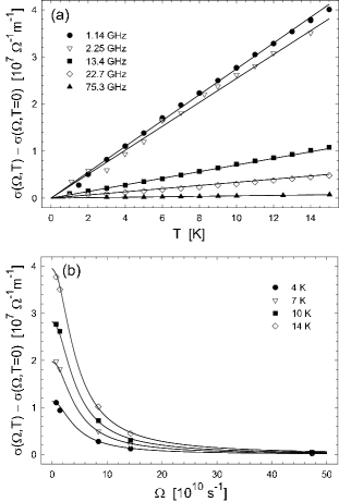
FIG. 6.: Fits to experiment of thermal regime microwave conductivity plotted (a) versus temperature for each of five frequencies and (b) versus frequency for each of four temperatures. Points denote the temperature-dependent part of the microwave conductivity measured in YBa₂Cu₃O_6.993 by Hosseini et al. [3] Lines denote a two parameter fit of Eq. (116) obtained with transport lifetime, $\tau_{tr}=2.93\times 10^{-11}$s, and Fermi-liquid renormalization factor, $\alpha_{fl}^{2}=0.6$.

However, there are several features of the Hosseini data that are not captured by Eq. (116). First of all, for each of the frequencies at which data was taken, a temperature-independent shift was observed in addition to the temperature-dependent part plotted in Fig. 6. Yet in our thermal regime expression, $\sigma(\Omega,T=0)$ is zero. Furthermore, though predominantly linear with temperature, the measured data deviates slightly, but noticeably, from linearity. In fact, Hosseini et al. note a gradual evolution from a concave-down (sub-linear) deviation at low frequencies to a concave-up (super-linear) deviation at high frequencies. Our thermal regime expression is strictly linear with temperature.

From the measured data (see Fig. 4 of Ref. [3]), it seems clear that the observed concave-down deviation at low frequencies results from the influence of inelastic scattering. For these low frequencies, the conductivity peak marking the onset of inelastic scattering appears just beyond the upper bound of our temperature range of interest. Quite naturally, the onset of inelastic scattering decreases the conductivity and yields a concave-down deviation from linearity. As we are concerned here with the nature of the low temperature elastic scattering mechanism, we do not expect to reproduce this feature. However, the observed high frequency (concave-up) deviations from linearity, as well as the temperature-independent shifts, do appear to be features of the elastic scattering which we seek to understand.

Since Eq. (116) is an approximate result, obtained by taking the limit $1/\tau,\Omega\ll T$ and thereby neglecting sub-dominant terms, it is possible that sub-dominant features (constant shift and deviation from linearity for high frequencies) were neglected when we assumed the thermal limit to obtain our analytical result. To see if these features emerge in an exact solution, we present numerical results, valid beyond the thermal limit, in the following section.

B Numerical Results

Recall from Sec. IV that the self-energy in the presence of line defect scattering is determined by the self-consistent solution of Eq. (22) as a function of momentum and energy. While an analytic expression was obtained in the thermal limit, this equation must be solved numerically for more general parameter values. Doing so (via Newton’s method) yields the self-energy functions, $\Sigma(p,\omega)$ and $\Sigma_{1}(p,\omega)$. Plugging these functions into Eqs. (75), (77), (93), (97), and (102) and numerically integrating over momentum and energy, we obtain the microwave conductivity for a particular temperature and frequency. Repeating this process for all temperatures and frequencies of interest yields an exact (numerical) result for the microwave conductivity.

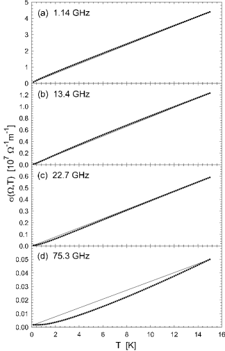
FIG. 7.: Results of exact numerical calculation of microwave conductivity plotted as a function of temperature for (a) 1.14 GHz, (b) 13.4 GHz, (c) 22.7 GHz, and (d) 75.3 GHz. Straight lines connecting the first and last data points have been included to highlight any deviation from linearity.

Following this procedure, we computed the microwave conductivity as a function of temperature, from 0 to 15 K, for each of the five experimentally relevant frequencies. In all cases, we used values of the transport lifetime and Fermi-liquid correction factor obtained, in the previous section, from the fit of our thermal regime expression to experiment. The results for 1.14 GHz, 13.4 GHz, 22.7 GHz, and 75.3 GHz are plotted versus temperature in Fig. 7. In each plot, a straight line has been drawn between the first and last data points to highlight any deviation from linearity. These exact results confirm the conclusions of our thermal regime calculation, revealing a predominantly linear temperature-dependence and a near-Drude frequency dependence. In addition, at the high frequencies where our thermal regime approximations were least justified, we obtain, in qualitative agreement with experiment, concave-up deviations from linearity. Furthermore, these results do exhibit nonzero, albeit very small, offsets at zero temperature (most evident for 75.3 GHz). However, the computed offsets are far smaller than those observed experimentally. Perhaps the point defect scattering, which is certainly present but was ignored herein for simplicity, is required to reproduce this feature correctly. A more complete calculation must consider the effects of both extended linear defects and point defects in the same system. This is an important direction for future study.

VII Conclusions

The low temperature behavior of the microwave conductivity measured in YBa₂Cu₃O_6.993 by Hosseini et al. [3] has been difficult to explain in terms of point defect (impurity) scattering. The basic problem is that the strong energy dependence of the low temperature quasiparticle density of states is directly reflected in a point defect scattering rate which is too energy dependent to produce a microwave conductivity that agrees with experiment. This suggests that an additional low temperature scattering mechanism may also be important.

We note that extended linear defect scattering is an appealing candidate. Unlike point defect scattering, line defect scattering does not sample the full quasiparticle density of states, so the line defect scattering rate need not inherit a strong energy dependence. Furthermore, lines are prevalent in as-grown YBCO in the form of twin boundaries. Although these twin boundaries are eliminated via the application of a uniaxial stress, if remnants of the twinning structure are left behind, they could take the form of line defects.

We have calculated (within the Born approximation) the self-energy and microwave conductivity due to scattering from a single domain of parallel, randomly spaced line defects, all aligned at $-45^{\circ}$ to the crystal axes. We find that the anisotropic nature of line defect scattering clearly differentiates odd nodes (for which electrical current is perpendicular to the defect lines) from even nodes (for which electrical current is parallel to defect lines). For the former, both intra-node (forward) scattering and opposite-node (back) scattering are permitted, whereas for the latter, only intra-node (forward) scattering is allowed. By including vertex corrections in our calculation, we have accounted for the fact that back scattering is an effective means of degrading a current while forward scattering is not. Therefore, while odd nodes yield a nonzero transport scattering rate and microwave conductivity, even nodes make no contribution. The resulting conductivity tensor is anisotropic, reflective of the anisotropic nature of the scattering mechanism. Thus, for a sample in which all twin boundaries were parallel prior to detwinning, this anisotropy should be observable. (In fact, the measurement of the conductivity tensor in such a single-domain sample would serve as a good test for the presence of line defects.) However, since the samples in question contain multiple domains with line defects aligned at $\pm 45^{\circ}$, we average over oppositely aligned domains to recover a conductivity scalar.

In the experimentally relevant limit, $1/\tau,\Omega\ll T\ll\Delta_{0}$, which we have called the thermal regime, our calculations simplify and we obtain an analytic expression for the microwave conductivity:

$$\tensor{\sigma}(\Omega,T)=\frac{e^{2}}{\pi^{2}}\frac{v_{f}}{v_{2}}2\ln(2)f(\Omega\tau_{tr}^{o})\frac{\tau_{tr}^{o}}{1+(\Omega\tau_{tr}^{o})^{2}}k_{B}T\tensor{\openone}.$$ (117)

As this result exhibits a linear temperature dependence and a near-Drude lineshape (modified logarithmically by the function $f(x)$ defined in Eq. (109)), it captures the most robust qualitative features of the Hosseini data. Furthermore, when we fit this expression to the temperature-dependent part of the measured conductivity (see Sec. VI A), we obtain good quantitative agreement with reasonable values of our two fitting parameters, the transport lifetime and the Fermi-liquid renormalization factor. However, we note that this approximate analytical result fails to reproduce the more subtle features of the measured data: temperature-independent offsets and deviations of the temperature dependence from strict linearity at high frequencies. (We note that the deviations observed at low frequencies can be explained by the onset of inelastic scattering.)

In search of these subdominant features, we performed an exact numerical calculation, valid beyond the thermal regime. These numerical results (see Sec. VI B) do exhibit deviations from linear temperature dependence at high frequencies, in qualitative agreement with experiment. While small temperature-independent offsets are also obtained, the magnitude of these is far smaller than observed experimentally. Perhaps the point defect scattering, which we have neglected herein, must be included to reproduce this feature.

The close agreement of our calculated conductivity with experiment strongly suggests that extended linear defects are indeed present in detwinned single crystals of YBa₂Cu₃O_6.993 and make an important contribution to the scattering. Our picture has been that these line defects are remnants of the twin boundary structure of the as-grown crystal, left behind after detwinning. We described, in Sec. III, a detwinning scenario whereby the annihilation of twin boundaries leaves behind lines of oxygen vacancies in the CuO layer. While this is one example of a process that could yield extended linear defects, others are certainly possible. Our results, however, imply that something similar to this is taking place.

To answer remaining questions and provide a more complete picture of the low temperature scattering, future calculations should include the effects of both line defect scattering and point defect scattering in the same system. Nevertheless, these initial results suggest that scattering from extended linear defects has a significant influence on the observed microwave conductivity in detwinned single crystals of YBa₂Cu₃O_6.993.

- [1] P. A. Lee, Science 277, 50 (1997)
- [2] J. Orenstein and A. J. Millis, Science 288, 468 (2000)
- [3] A. Hosseini, R. Harris, S. Kamal, P. Dosanjh, J. Preston, R. Liang, W. N. Hardy, and D. A. Bonn, Phys. Rev. B 60, 1349 (1999)
- [4] D. A. Bonn, S. Kamal, A. Bonakdarpour, R. Liang, W. N. Hardy, C. C. Homes, D. N. Basov, and T. Timusk, Czech. J. Phys. 46, 3195 (1996)
- [5] S. F. Lee, D. C. Morgan, R. J. Ormeno, D. M. Broun, R. A. Doyle, J. R. Waldram, and K. Kadowaki, Phys. Rev. Lett. 77, 735 (1996)
- [6] D. A. Bonn, R. Liang, T. M. Riseman, D. J. Baar, D. C. Morgan, K. Zhang, P. Dosanjh, T. L. Duty, A. MacFarlane, G. D. Morris, J. H. Brewer, W. N. Hardy, C. Kallin, and A. J. Berlinsky, Phys. Rev. B 47, 11314 (1993)
- [7] D. A. Bonn, P. Dosanjh, R. Liang, and W. N. Hardy, Phys. Rev. Lett. 68, 2390 (1992)
- [8] P. J. Hirschfeld, W. O. Putikka, and D. J. Scalapino, Phys. Rev. Lett. 71, 3705 (1993)
- [9] P. J. Hirschfeld, W. O. Putikka, and D. J. Scalapino, Phys. Rev. B 50, 10250 (1994)
- [10] P. J. Hirschfeld, P. Wölfe, J. A. Sauls, D. Einzel, and W. O. Putikka, Phys. Rev. B 40, 6695 (1989)
- [11] P. J. Hirschfeld, D. Vollhardt, and P. Wölfe, Solid State Comm. 59, 111 (1986)
- [12] H. Monien, K. Scharnberg, and D. Walker, Solid State Comm. 63, 263 (1987)
- [13] P. J. Hirschfeld, P. Wölfe, and D. Einzel, Phys. Rev. B 37, 83 (1988)
- [14] M. J. Graf, M. Palumbo, D. Rainer, and J. A. Sauls, Phys. Rev. B 52, 10588 (1995)
- [15] Y. Sun and K. Maki, Europhys. Lett. 32, 355 (1995)
- [16] M. B. Walker and M. F. Smith, Phys. Rev. B 61, 11285 (2000)
- [17] A. J. Berlinksy, D. A. Bonn, R. Harris, and C. Kallin, Phys. Rev. B 61, 9088 (2000)
- [18] Note that this is the limit opposite to that known as the “universal” limit (). [P. A. Lee, Phys. Rev. Lett. 71, 1887 (1993)]
- [19] Note that Hettler and Hirschfeld have recently proposed a more complex theory of impurity scattering, involving order parameter suppression at impurity sites, to fit the experimental data using a point defect model. [M. H. Hettler and P. J. Hirschfeld, Phys. Rev. B 61, 11313 (2000) and Phys. Rev. B 59, 9606 (1999)]
- [20] R. Harris, (private communication)
- [21] H. Shaked, P. M. Keane, J. C. Rodriguez, F. F. Owen, R. L. Hitterman, and J. D. Jorgensen, Crystal Structures of the High- Superconducting Copper-Oxides (Elsevier Science B. V., Amsterdam, The Netherlands 1994)
- [22] J. L. Tallon, Phys. Rev. B 39, 2784 (1989)
- [23] A. C. Durst and P. A. Lee, Phys. Rev. B 62, 1270 (2000)
- [24] P. A. Lee and X. G. Wen, Phys. Rev. Lett. 78, 4111 (1997)
- [25] M. Chiao, R. W. Hill, C. Lupien, and L. Taillefer, Phys. Rev. B 62, 3554 (2000); L. Taillefer, Bull. Am. Phys. Soc. 46, 363 (2001)
- [26] A. J. Millis, S. M. Girvin, L. B. Ioffe, and A. I. Larkin, J. Phys. Chem. Solids 59, 1742 (1998)
- [27] J. Mesot, M. R. Norman, H. Ding, M. Randeria, J. C. Campuzano, A. Paramekanti, H. M. Fretwell, A. Kaminski, T. Takeuchi, T. Yokoya, T. Sato, T. Takahashi, T. Mochiku, and K. Kadowaki, Phys. Rev. Lett. 83, 840 (1999)
- [28] D. Xu, S. K. Yip, and J. A. Sauls, Phys. Rev. B 51, 16233 (1995)
- [29] K. Zhang, D. A. Bonn, S. Kamal, R. Liang, D. J. Baar, W. N. Hardy, D. Basov, and T. Timusk, Phys. Rev. Lett. 73, 2484 (1994)