Lamellar phase stability in diblock copolymers under reciprocating shear flows

Abstract

A mesoscopic model of a diblock copolymer is used to study the stability of a uniform lamellar phase under a reciprocating shear flow. Approximate viscosity contrast between the microphases is allowed through a linear dependence of the (Newtonian) shear viscosity on monomer composition. We first show that viscosity contrast does not affect the composition of the base lamellar phase in an unbounded geometry, and that it only couples weakly to long wavelength perturbations. A perturbative analysis is then presented to address the stability of uniform lamellar structures under long wavelength perturbations by self-consistently solving for the composition and velocity fields of the perturbations. Stability boundaries are obtained as functions of the physical parameters of the polymer, the parameters of the flow and the initial orientation of the lamellae. We find that all orientations are linearly stable within specific ranges of parameters, but that the perpendicular orientation is generally stable within a larger range than the parallel orientation. Secondary instabilities are both of the Eckhaus type (longitudinal) and zig-zag type (transverse). The former is not expected to lead to re-orientation of the lamella, whereas in the second case the critical wavenumber is typically found to be along the perpendicular orientation.

1 Introduction

Diblock copolymers are macromolecules comprising two chemically distinct and mutually incompatible segments (monomers) that are covalently bonded. The equilibrium properties are determined by the degree of polymerization $N$, (i.e., the length of the polymer chain), the volume fraction of one of the monomers $f$, and the Flory-Huggins interaction parameter between the distinct segments $\chi$ [1, 2]. While the degree of polymerization and the monomer volume fraction are determined by the processing conditions, the value of the parameter $\chi$ is entirely determined by the choice of monomers and temperature.

Above the order-disorder transition temperature $T_{ODT}$, the equilibrium phase is disordered and the monomer concentration uniform. In mean field theory, the order-disorder transition takes place at $\chi N\simeq 10$, where the Flory-Huggins parameter and temperature $T$ are related through $\chi=\alpha/T+\beta$, where $\alpha>0$ and $\beta$ are two constants [1]. Below $T_{ODT}$, equilibrium structures of a wide variety of symmetries have been predicted and experimentally observed [3]. Around $f=0.5$ (symmetric mixture), a so called lamellar phase is observed, in which nanometer sized layers of A and B rich regions alternate in space. When the copolymer is quenched from a high temperature to a temperature $T<T_{ODT}$, a transient polycrystalline configuration results comprising many lamellar domains (or grains), with lamellar normals of arbitrary orientations. In practice, full development of the equilibrium state requires very long annealing times until substantial long ranged order at the scale of the system size can be achieved. However, the underlying ordering mechanisms and associated rates that contribute to the large scale reorientation of the grains are essentially unknown at present. Not only partial ordering is detrimental for some applications, but it can also lead to aging of the material, as well as to potentially anomalous response to applied stresses. We present below our analysis of one of the possible mechanisms contributing to the kinetics of large scale reorientation of lamellar domains, especially in connection with the use of reciprocating shears to accelerate grain coarsening.

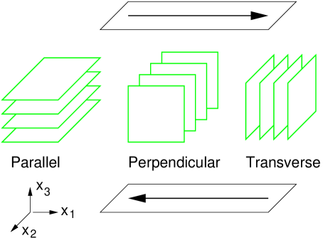
Figure 1: Schematic representation of the geometry considered including the shear direction, and the three different lamellar orientations discussed in the text.

Imposing a reciprocating shear is one of the methods currently in use to achieve long-ranged order of block copolymer microstructures. Early work on the response of block copolymer blends to shears [4, 5, 6] aimed at establishing the dependence of $T_{ODT}$ on the shear rate, but the experiments also revealed that the shear helped select specific lamellar orientations. These observations have subsequently led to a large number of groups attempting to quantify the type and degree of ordering that can be achieved by reciprocating shears. Early experiments by Koppi et al. [5, 6] involved the copolymer poly-(ethylene-propylene) - poly-(ethylethylene) (PEP-PEE). Upon lowering the temperature below $T_{ODT}$, they observed a transition to the so-called parallel lamellae at moderate shear rates, but also an unexpected transition to perpendicular lamellae at high frequencies (in parallel alignment, the layers are normal to the shear gradient direction, whereas in perpendicular alignment the layers are normal to the vorticity direction; see a schematic representation in Fig. 1). It was also possible to induce the transition from parallel to perpendicular by increasing the shear frequency, but this transformation was not reversible. Koppi et al. interpreted the high frequency behavior as shear disordering of the original configuration, followed by formation of the perpendicular orientation. Instead, the parallel orientation was argued to result from defect mediated growth.

This phenomenology is qualitatively consistent with the most complete theoretical analysis to date due to Fredrickson [7], although one must note that his results were obtained for steady shears instead. He used the same model equations that we use below in our study, but explicitly allowed for thermal fluctuations near $T_{ODT}$, as he was primarily interested in modeling orientation selection at $T_{ODT}$ through anisotropic fluctuation suppression by the shear flow. He approximated the effect of the flow by introducing a modified order parameter mobility that depended on the integrated flow over the volume of the sample. Given the inverse characteristic decay time of concentration fluctuations, $\dot{\gamma}^{*}$, he showed that for shear rates $\dot{\gamma}<\dot{\gamma}^{*}$ the parallel orientation is preferred. In the opposite limit, the first transition upon lowering the temperature leads to a perpendicular orientation. Further decrease in temperature led to transition back to a parallel structure. The range of existence of the perpendicular orientation was argued to decrease with increasing viscosity contrast between the two microphases.

However, the phenomenology just described is exactly reversed for a poly-(styrene) - poly-(isoprene) (PS-PI) copolymer. Here the perpendicular orientation is observed at low frequencies, and the parallel orientation at large frequencies [8, 9]. There is disagreement in the results at low frequencies, as Wiesner and coworkers find a parallel orientation at low frequency [10, 11] in the same range investigated by others. The experimental results have been summarized in [12]: for frequencies $\omega<\omega_{d}$ a parallel orientation has been found in two out of four studies. At intermediate frequencies $\omega_{d}<\omega<\omega_{c}^{\prime}$ the preferred orientation is perpendicular, whereas for $\omega>\omega_{c}^{\prime}$ the observed orientation is parallel. The frequency $\omega_{d}$ is a characteristic inverse time of local domain deformation, and $\omega_{c}^{\prime}$ is a frequency above which chain relaxation dynamics dominates the storage modulus $G^{\prime}(\omega)$.

A different line of theoretical investigation has shifted the focus of study away from fluctuations at $T_{ODT}$ and into secondary instabilities of a well developed lamellar pattern [13, 14, 15]. Kodama and Doi [13] used a cell dynamical model to study possible instabilities of a lamellar pattern upon shearing. The numerical results obtained motivated in turn an analytic stability analysis that, now in the absence of flow, addressed lamellar stability against a change in wavelength. Shiwa [14] later investigated the similarity between the amplitude or envelope equations describing slow modulations of a lamellar structure and the same equations describing roll distortions in Rayleigh-Bénard convection. In the limit of vanishing shear amplitude, he established the equivalence of the stability diagram of both systems, and hence inferred the range of stability of a lamellar phase against Eckhaus (longitudinal) and zig-zag (transverse) instabilities. We were later able to obtain lamellar solutions under uniform steady and oscillatory shears of finite amplitude [15], and to study their stability. Stability boundaries of the base lamellar phase against both melting and long wavelength perturbations were obtained for transverse and parallel orientations. However, we did not address the perpendicular orientation, nor the effect of viscosity contrast on the stability diagram. The consideration of both a full three dimensional geometry and viscosity contrast are the subject matters of this paper.

We present a full three dimensional stability analysis of a uniform lamellar phase under a reciprocating shear flow with an assumed linear dependence of the shear viscosity on local monomer composition. We self-consistently determine the velocity field and monomer composition and study the growth or decay of long wavelength perturbations of a base lamellar phase. The stability analysis leads to a Floquet problem for the perturbation amplitudes, which we solve numerically. First, we find that viscosity contrast has a negligible effect on the stability boundaries of the lamellar phase. Second, from the actual computation of these boundaries we find that, in general, the region of stability is larger for the perpendicular rather than the parallel orientation. Third, the marginal mode for the transverse instability branch is typically along the perpendicular orientation, so that the initial decay of both parallel and transverse uniform states would lead to the appearance of a perpendicular component. We finally show that the orientation of the marginal mode of instability can be generally understood from geometrical considerations. At a zig-zag boundary, for example, the marginal mode tends to be oriented along the direction that causes the largest decrease in lamellar wavelength by the shear.

2 Mesoscopic model equations and lamellar phases

At a mesoscopic level, a block copolymer melt is described by an order parameter $\psi({\bf r})$ which represents the local density difference between the two monomers constituting the copolymer. The corresponding free energy was derived by Leibler [16] in the weak segregation limit (close to $T_{ODT}$), and later extended by Ohta and Kawasaki [17] to the strong segregation regime. If the temporal evolution of $\psi$ occurs through advection by a flow field as well as through local dissipation driven by free energy reduction, $\psi$ obeys a time dependent Ginzburg-Landau equation [18, 7],

$$\frac{\partial\psi}{\partial t}+({\mathbf{v}}\cdot\nabla)\psi=M\nabla^{2}(-r\psi+u\psi^{3}-K\nabla^{2}\psi)-MB\psi.$$ (1)

with ${\bf v}$ the velocity, $B$ a parameter that characterizes the amplitude of the long ranged interactions arising from the covalent bond connecting the two sub-chains [17], and $M$ a phenomenological mobility or Onsager coefficient [3]. The remaining parameters appearing in the equation can be related to physical properties of the polymer chains as follows [13]: $K=b^{2}/3$, where $b$ is Kuhn’s statistical length of the chain, $r=(2\chi N-7.2)/N$, and $B=144/N^{2}b^{2}$.

Under the assumption of Newtonian behavior, the equation governing the velocity field is an extended Navier-Stokes equation for an incompressible fluid,

$$\rho_{0}\frac{\partial\mathbf{v}}{\partial t}+\rho_{0}({\mathbf{v}}\cdot{\mathbf{\nabla}}){\mathbf{v}}=\nabla\cdot\left[\eta\left(\nabla{\mathbf{v}}+\nabla{\mathbf{v}}^{T}\right)\right]-{\mathbf{\nabla}}p+\frac{\delta{\cal F}}{\delta\psi}{\mathbf{\nabla}}\psi,\quad\nabla\cdot{\mathbf{v}}=0,$$ (2)

where $\rho_{0}$ is the (constant) density, $\eta$ the shear viscosity of the fluid which may depend on $\psi$, $p$ is the pressure, and appropriate boundary conditions for both $\psi$ and v must be introduced. The last term on the right-hand side of Eq. (2) is required to ensure that there cannot be free energy reduction by pure advection of $\psi$ [19]. This term leads to the creation of rotational flow by curved lamellae that is directed toward their local center of curvature.

We first introduce dimensionless variables following ref. [15]. Lengths are scaled by $\sqrt{K/r}$ which is proportional to the lamellar wavelength, time by $K/Mr^{2}$, the characteristic monomer diffusion time, and order parameter $\psi$ by $\sqrt{r/u}$. As described in that reference, only one dimensionless group remains in Eq. (1), $B^{\prime}=BK/r^{2}$. In dimensionless units (we also omit the prime in $B$; it is assumed to be a dimensionless coefficient in what follows), Eq. (1) reads,

$$\frac{\partial\psi}{\partial t}+({\mathbf{v}}\cdot\nabla)\psi=\nabla^{2}(-\psi+\psi^{3}-\nabla^{2}\psi)-B\psi.$$ (3)

The mean field order-disorder transition occurs at $B_{c}=1/4$ with a critical wavenumber $q_{c}=\sqrt{1/2}$.

Equation (2) can be further simplified by noting that the order parameter diffusivity (proportional to of $Mr$) is much smaller than the kinematic viscosity $\eta/\rho_{0}$, and that under typical experimental conditions $\rho_{0}\omega d/\eta\ll 1$ as well, where $\omega$ is the angular frequency of the oscillatory shear, and $d$ the thickness of the block copolymer layer. We therefore adopt a creeping flow approximation according to which the flow field instantaneously relaxes to that determined by the instantaneous configuration of the order parameter $\psi$ (and the no-slip boundary conditions). We further neglect in our present study the term $\frac{\delta{\cal F}}{\delta\psi}{\mathbf{\nabla}}\psi$ in the right hand side of Eq. (2). Therefore the only dependence of this equation on the order parameter $\psi$ enters though the shear viscosity $\eta=\eta(\psi)$, as we focus on the effect of viscosity contrast between the microphases on the stability of a lamellar structure.

An important restriction of our calculations is that the fluid remains Newtonian. This is in line with previous calculations on this system, but it is an approximation that needs to be removed in future work, as already noted in the introduction. We consider here a specific linear dependence of the shear viscosity on $\psi$,

$$\eta=\eta_{0}+\eta_{1}\psi,$$ (4)

where $\eta_{1}$ does not have to be small compared to $\eta_{0}$. Within the approximation stated, and in dimensionless variables, Eq. (2) reduces to,

$$0=\nabla p+\nabla\left[\left(1+\eta_{1}\psi\right)\left(\nabla{\mathbf{v}}+\nabla{\mathbf{v}}^{T}\right)\right],$$ (5)

where the dimensionless viscosity correction $\eta_{1}^{\prime}=\sqrt{r/u}(\eta_{1}/\eta_{0})$ has been introduced (and the prime removed).

The physical system under consideration is a layer of block copolymer, unbounded in the $x_{1}$ and $x_{2}$ directions, and being uniformly sheared along the $x_{3}$ direction (Fig. 1). The layer is confined between the stationary $x_{3}=0$ plane, and the plane $x_{3}=d$ which is uniformly displaced parallel to itself with a velocity ${\mathbf{v}}_{\mathrm{plane}}=\gamma\,d\,\omega\,\cos(\omega t)\hat{\bf x}_{1}$, where $\hat{\bf x}_{1}$ is the unit vector in the $x_{1}$ direction. $\gamma$ is the dimensionless strain amplitude and $\omega$ is the angular frequency of the shear. In what follows, this velocity is also expressed in the dimensionless variables given above. In particular, the dimensionless wall velocity can be written as ${\mathbf{v}}_{\mathrm{plane}}^{\prime}=\gamma^{\prime}\cos(\omega^{\prime}t^{\prime})$ so that with the scalings introduced earlier, $\gamma^{\prime}=\sqrt{2}(\omega\tau_{D})(q_{c}d)\gamma$, with $\tau_{D}=K/Mr^{2}$ the (diffusion) time scale introduced earlier. Since for a realistic system $q_{c}d\gg 1$, the relatively small values of $\gamma^{\prime}$ required for instability (see below) implies that our study addresses in practice shear frequencies much smaller than the inverse diffusion time. Again, in what follows we restrict ourselves to dimensionless variables and drop the primes.

We first summarize the results of ref. [15] in which the viscosity was assumed uniform. We focused there on the weak segregation limit $\epsilon=(B_{c}-B)/2B_{c}\ll 1$, in which the solution for the monomer composition can be obtained perturbatively in $\epsilon$,

$$\psi({\mathbf{r}})=2A(t)\cos({\mathbf{q}}\cdot{\mathbf{r}})+A_{1}(t)\cos(3{\mathbf{q}}\cdot{\mathbf{r}})+\ldots$$ (6)

where ${\mathbf{r}}=x_{1}\hat{\bf x}_{1}+x_{2}\hat{\bf x}_{2}+x_{3}(\gamma\sin(\omega t)\hat{\bf x}_{1}+\hat{\bf x}_{3})$ so that it can be thought of as having components in a non orthogonal basis set which follows the imposed shear, and ${\mathbf{q}}=(q_{1},q_{2},q_{3})$ is the wavevector in the corresponding reciprocal space basis set $\{{\mathbf{g}}_{1}=\hat{\bf x}_{1}-\gamma\sin(\omega t)\hat{\bf x}_{3},{\mathbf{g}}_{2}=\hat{\bf x}_{2},{\mathbf{g}}_{3}=\hat{\bf x}_{3}\}$. Note that in this new coordinate system, perfectly ordered configurations are stationary. Three orientations relative to the shear can be defined as follows: $q_{3}\neq 0,q_{1}=q_{3}=0$ is a purely parallel orientation, $q_{2}\neq 0,q_{1}=q_{3}=0$ is a perpendicular orientation, and $q_{1}\neq 0,q_{2}=q_{3}=0$ is a transverse orientation.

In the absence of viscosity contrast, the velocity field is given by,

$${\mathbf{v}}^{0}=\gamma\omega\cos(\omega t)\;x_{3}\;\hat{\bf x}_{1}.$$ (7)

Furthermore, by substituting Eq. (6) into Eq. (3), the lowest order solution (${\cal O}(\epsilon^{1/2})$) is given by

$$\psi({\mathbf{r}})=2A(t)\cos({\mathbf{q}}\cdot{\mathbf{r}})$$ (8)

where the amplitude $A(t)$ satisfies the equation [15],

$$\frac{dA}{dt}=\sigma[q^{2}(t)]A-3q^{2}(t)A^{3},$$ (9)

with $q^{2}(t)=q_{1}^{2}+[\gamma\sin(\omega t)q_{1}-q_{3}]^{2}+q_{2}^{2}$ and $\sigma(q^{2})=q^{2}-q^{4}-B$. This equation can be integrated to give the marginal stability boundaries, and the function $A(t)$ itself [15]. From this analysis, a critical strain amplitude $\gamma_{c}$, which depends on ${\bf q}$, was identified such that for $\gamma<\gamma_{c}$ the uniform lamellar structure oscillates with the imposed shear, but at $\gamma>\gamma_{c}$ $A(t)$ decays to zero; i.e., the lamellar structure melts, to use the terminology used in experiments.

The stability of the base lamellar pattern was then addressed in two spatial dimensions by a Floquet analysis. The study was restricted to the $(x_{1},x_{3})$ plane (i.e., $q_{2}=0$), and therefore restricted to transverse ($q_{3}=0$) and parallel ($q_{1}=0$) lamellae only. Briefly, for sufficiently small $\gamma$ all orientations were seen to retain a range of stability in wavenumber, range that becomes narrower along the diagonal in the $(q_{1},q_{3})$ plane. The range of stability is further reduced with increasing frequency. At moderate shear amplitudes (e.g., $\gamma=0.4$), only fully parallel or transverse lamellae remain stable, and there is also a weak frequency dependence. We extend below these results to three spatial dimensions and to a fluid with a nonuniform shear viscosity, function of the local monomer composition $\psi$. Our aim is to incorporate into the stability analysis a different effective rheology of the two microphases.

3 Stability of a lamellar phase under shear

We obtain in this section the flow in the melt that arises from the nonuniform shear viscosity, and the resulting corrections to the base lamellar solution. We then perform a self-consistent stability analysis of the lamellar order parameter and flow field against long wavelength perturbations.

There is now ample evidence that viscoelastic contrast between the microphases affects orientation selection. We wish to investigate here whether such a contrast substantially affects the stability of a uniform lamellar phase to shear. This is an initial step in attempting to understand the experimental phenomenology. For example, and as briefly discussed in Section 1, the qualitative response to oscillatory shears in a system such as poly-(ethylene-propylene) - poly-(ethylethylene) (PEP-PEE) is qualitatively very different than that of, say, poly-(styrene) - poly-(isoprene) (PS-PI). The former prefers the parallel orientation at low frequencies and the perpendicular orientation at higher frequencies, whereas the behavior is essentially reversed for the latter. As emphasized by Fredrickson and Bates [3], the microphases of the PEP-PEE system are well matched mechanically. However, PS is largely unentangled whereas PI is entangled. Therefore a large contrast in the relaxation times of the blocks is anticipated. Also recent experimental evidence by Winey and coworkers [20] suggests that the response of a parallel configuration to shear can be qualitatively described by a three region model. One central region in the vicinity of the covalent bond between the A and B chains is relatively stiff, and responds elastically under shear. This region is surrounded by two other regions with a largely viscous response to the shear as the chains are elongated. Before addressing the more general case of viscoelastic contrast between the microphases, we study in this paper a fairly simplistic situation in which the blend remains a Newtonian fluid, but one in which the shear viscosity depends explicitly on the local monomer composition $\eta=\eta(\psi)$, and hence the actual flow field inside the melt depends on the order parameter configuration. We follow a related study by Fredrickson [7] who incorporated viscosity contrast by computing an averaged, effective shear rate for a lamellar configuration, which then renormalized the mobility coefficient in the time dependent Ginzburg-Landau equation for the order parameter. We do consider here, however, the full calculation of the flow field self-consistently, although for practical convenience we restrict our analysis to the linear variation given in Eq. (4). In this case, we can solve for the base flow field exactly, fact that considerably simplifies the stability analysis.

We begin by writing Eq. (5) in components,

$$\partial_{i}p-\partial_{j}[(1+\eta_{1}\psi)(\partial_{i}v_{j}+\partial_{j}v_{i})]=0,$$ (10)

and consider periodic boundary conditions along the $\hat{\bf x}_{1}$ and $\hat{\bf x}_{2}$ directions. To facilitate the computation, we replace no slip boundary conditions in the $\hat{\bf x}_{3}$ direction by sheared periodic boundary conditions (i.e., periodic boundary conditions in a frame of reference rigidly attached to the moving plates. See, e.g., ref. [15] for further details). We then introduce the decomposition

$${\bf v}={\bf v}^{0}+{\bf u}.$$ (11)

The governing equation for the velocity ${\bf u}$ is (with $\psi({\bf r})=2A\cos({\bf q}\cdot{\bf r})$)

$$-\partial_{i}p_{1}+\partial_{j}[(1+\eta_{1}\psi)(\partial_{i}v^{0}_{j}+\partial_{j}v^{0}_{i})]+\partial_{j}[(1+\eta_{1}\psi)(\partial_{i}u_{j}+\partial_{j}u_{i})]=0$$ (12)

In order to solve this equation, we introduce a new set of coordinates $(x^{\prime},y^{\prime},z^{\prime})$ such that $\hat{z^{\prime}}=\hat{\bf q}$ (the $z^{\prime}$ direction is parallel to the time dependent wavevector of the lamellar phase), and $\hat{y^{\prime}}$ is perpendicular to the plane $(q_{z},0,q_{x})$. Then $u_{y^{\prime}}$ and $u_{z^{\prime}}$ vanish in the lamellar phase, and the equation for $u_{x^{\prime}}$, after some algebra, is given by,

$$\partial_{z^{\prime}}[(1+2\eta_{1}A(t)\cos qz^{\prime})\partial_{z^{\prime}}u_{x^{\prime}}]=\gamma\eta_{1}A(t)q\beta\sin qz^{\prime},$$ (13)

with $\beta=2[-(q_{x}^{2}-q_{z}^{2})^{2}-q_{y}^{2}(q_{x}^{2}+q_{z}^{2})]/qn_{x}$ and $n_{x}=|(q_{z}(q_{x}^{2}-q_{y}^{2}-q_{z}^{2}),2q_{x}q_{y}q_{z},$ $-q_{x}(q_{x}^{2}+q_{y}^{2}-q_{z}^{2}))|$, where the wavevector ${\mathbf{q}}$ is a function of time as the orientation of the base lamellar structure adiabatically follows the imposed shear flow. Equation (13) can now be integrated twice to obtain $u_{x^{\prime}}$. It is important to note that for a purely perpendicular base state $\beta=0$, and hence the flow correction ${\bf u}=0$ in this case. This is in agreement with the results of Fredrickson [7].

A general property of the solution for the flow perturbation ${\mathbf{u}}$ that follows from the linear form of the viscosity contrast is that the velocity is always perpendicular to ${\bf q}$, i.e., parallel to the lamellar planes which are the planes of constant $\psi$. Therefore the advection term ${\mathbf{u}}\cdot\nabla\psi=0$ for a lamellar phase, and hence the base field $\psi$ is unaffected by the flow. Note that this result is general as long as the order parameter is a function of one spatial direction only. In the more general cases, only the functional dependence in $\cos(z^{\prime})$ and $\sin(z^{\prime})$ in Eq. (13) would be different. In short, Eq. (8) remains the solution for the order parameter when the viscosity contrast is given by Eq. (4). The base flow field can be obtained from the solution of Eq. (13) and Eq. (11).

We next address the stability of the solution Eqs. (7) and (8) against long wavelength perturbations at fixed $\epsilon$ [21]. We consider solutions of the form

$$\psi = \psi_{1}+\psi_{2}$$

$${\bf v} = {\bf v}^{0}+{\bf u}+{\bf w}$$

where $\psi_{1}$ is the base solution given in Eq. (8), ${\mathbf{u}}$ the solution of Eq. (13), and,

$$\psi_{2}=\psi_{2+}\;e^{i{\bf q}\cdot{\bf r}+i{\bf Q}\cdot{\bf r}}+\psi_{2-}\;e^{i{\bf q}\cdot{\bf r}-i{\bf Q}\cdot{\bf r}}+\hbox{c.c.}$$ (14)

If the wavevector of the perturbation ${\bf Q}$ is parallel to the base wavevector ${\bf q}$, the perturbation is said to be of the Eckhaus type. In the case of ${\bf Q}\perp{\bf q}$, we are considering a zig-zag perturbation. Due to our choice of shear periodic boundary conditions, and unlike more standard analyses of long wavelength instabilities, the perturbation wavevector ${\bf Q}$ is time dependent and periodic with the same periodicity as the shear (the same is true for ${\bf q}$).

The stability of periodic solutions of the current model in the absence of flow has been extensively studied [22, 14]. There is a range of wavenumbers $q$ within which the lamellar states are stable. This range of stability increases with the distance to threshold $\epsilon$. At large wavenumbers, lamellae undergo an Eckhaus instability which tends to lowers the value of $q$ by eliminating lamellar layers. On the other hand, at small wavenumbers the wavenumber is increased via a zig-zag instability. As we show below, the imposed oscillatory shear has important consequences for these two instabilities, especially for the zig-zag case. In particular, we show that the way in which a zig-zag instability leads to a readjustment of the lamellar wavelength depends strongly on the relative orientation between the base lamellae and the shear direction.

In order to derive an evolution equation for the two amplitudes $\psi_{2+}$ and $\psi_{2-}$ we need the velocity field ${\bf w}$. Since the convective term in Eq. (1) is ${\bf v}\cdot\nabla\psi=({\bf u}+{\bf w})\cdot\nabla(\psi_{1}+\psi_{2})$, we only need to retain Fourier components of the form $e^{\pm i{\bf q}\cdot{\bf r}\pm i{\bf Q}\cdot{\bf r}}$. Therefore one only needs the Fourier components $e^{\pm 2i{\bf q}\cdot{\bf r}}$ for ${\bf u}$ and $e^{\pm 2i{\bf q}\cdot{\bf r}\pm i{\bf Q}\cdot{\bf r}}$ for ${\bf w}$. The governing equation for the second order velocity ${\bf w}$ reads,

$$-\partial_{i}p_{2}+\partial_{j}[(1+\eta_{1}\psi_{1})(\partial_{i}w_{j}+\partial_{j}w_{i})]\hskip 113.81102pt$$

$$~{}+\partial_{j}[\eta_{1}\psi_{2}(\partial_{i}u_{j}+\partial_{j}u_{i})]+\partial_{j}[\eta_{1}\psi_{2}(\partial_{i}v^{0}_{j}+\partial_{j}v^{0}_{i})] = 0.$$

This equation is solved by transforming again to the $(x^{\prime},y^{\prime},z^{\prime})$ coordinate system. The sum of the third and fourth terms is the inhomogeneous term in the equations and is of the form of ${\bf h}(qz^{\prime})e^{i{\bf Q^{\prime}}\cdot{\bf r}^{\prime}}+\hbox{c.c.}$. Therefore we write the second order velocity as

$${\bf w} = e^{i{\bf Q^{\prime}}\cdot{\bf r}^{\prime}}{\bf\overline{w}}(qz^{\prime})+\hbox{c.c.}$$

$$p_{2} = e^{i{\bf Q^{\prime}}\cdot{\bf r}^{\prime}}\overline{p}_{2}(qz^{\prime})+\hbox{c.c.}$$

which leads to the equations

$$-\partial_{i}\overline{p}_{2}(qz^{\prime})+(iQ^{\prime}_{j}+\partial_{j})[1+\eta_{1}\psi_{1}(qz^{\prime})]\times\qquad$$ (15)

$$[(iQ^{\prime}_{i}+\partial_{i})\overline{w}_{j}(qz^{\prime})+(iQ^{\prime}_{j}+\partial_{j})\overline{w}_{i}(qz^{\prime})] = h_{i}(qz^{\prime}).$$ (16)

We now solve for the functions ${\bf\overline{w}}(qz^{\prime})$ and $\overline{p}_{2}(qz^{\prime})$ numerically together with the incompressibility condition,

$$iQ_{x^{\prime}}\overline{w}_{x^{\prime}}+iQ_{y^{\prime}}\overline{w}_{y^{\prime}}+(iQ_{z^{\prime}}+\partial_{z^{\prime}})\overline{w}_{z^{\prime}}=0.$$ (17)

Since the velocity ${\bf w}$ is proportional to $\psi_{2}$, and given the latter’s decomposition in its components $e^{2i{\bf q}\cdot{\bf r}}$ and ^iQ⋅r, we find it useful to express ${\bf w}$ as

$${\bf w}=\left({\bf w}^{++}e^{2i{\bf q}\cdot{\bf r}}\psi_{2+}+{\bf w}^{+-}e^{-2i{\bf q}\cdot{\bf r}}\psi_{2+}+{\bf w}^{-+}e^{2i{\bf q}\cdot{\bf r}}\psi_{2-}^{*}+{\bf w}^{--}e^{-2i{\bf q}\cdot{\bf r}}\psi_{2-}^{*}\right)e^{i{\bf Q}\cdot{\bf r}}+\hbox{c.c.}$$

Also by considering the Fourier expansion of ${\bf u}$,

$${\bf u}={\bf u}_{1}e^{i{\bf q}\cdot{\bf r}}+{\bf u}_{2}e^{2i{\bf q}\cdot{\bf r}}+\cdots+\hbox{c.c.}$$

we arrive at the (linearized) system of equations obeyed by the perturbation $\psi_{2}$,

$$\frac{\partial}{\partial t}\left[\begin{array}[]{c}\psi_{2+}\\ \psi_{2-}^{*}\end{array}\right]=\left[\begin{array}[]{cc}H_{11}(t)&H_{12}(t)\\ H_{21}(t)&H_{22}(t)\end{array}\right]\left[\begin{array}[]{c}\psi_{2+}\\ \psi_{2-}^{*}\end{array}\right].$$ (18)

This is the central result of this section. The matrix elements are given by,

$$H_{11}(t) = -l_{+}-l_{+}^{2}+B+6A(t)^{2}l_{+}+iA(t){\bf w}^{++}\cdot{\bf q}$$

$$H_{12}(t) = 3A(t)^{2}l_{+}+iA(t){\bf w}^{-+}\cdot{\bf q}+i{\bf u}_{2}\cdot({\bf q}-{\bf Q})$$

$$H_{12}(t) = 3A(t)^{2}l_{-}-iA(t){\bf w}^{+-}\cdot{\bf q}-i{\bf u}_{2}\cdot({\bf q}+{\bf Q})$$

$$H_{22}(t) = -l_{-}-l_{-}^{2}+B+6A(t)^{2}l_{-}-iA(t){\bf w}^{--}\cdot{\bf q}$$

with $l_{\pm}=-({\bf q}+{\bf Q})^{2}$. First we note that the matrix elements are periodic in time, with the same periodicity as the imposed shear. Therefore the stability analysis constitutes a Floquet problem for the amplitudes $\psi_{2+}$ and $\psi_{2-}$ which we solve numerically. Briefly, the function $A(t)$ is evaluated numerically for a given lamellar orientation and shear flow parameters. The flow correction due to viscosity contrast ${\bf u}$ in the base state is known analytically, but the flow perturbation ${\bf w}$ is obtained numerically by solving Eqs. (16) and (17). Once the matrix elements in Eq. (3) have been numerically evaluated, the Floquet problem is recast as an eigenvalue problem, which is then solved numerically. For fixed $\epsilon,\gamma,\omega$ and $\eta_{1}$ the stability boundaries are determined as the loci of ${\bf q}$ at which the eigenvalue function $\sigma({\bf Q})$ changes from a maximum to a saddle point at ${\bf Q}=0$.

We finally note that the fact that the Floquet problem only involves the amplitudes $\psi_{2+}$ and $\psi_{2-}$ and not ${\bf w}^{++},{\bf w}^{+-},{\bf w}^{-+}$ and ${\bf w}^{--}$ is a direct consequence of the creeping flow approximation introduced: the velocity field is slaved to the composition field.

4 Results and discussion

As illustrated in Fig. 1 and discussed in Section 1, the configuration considered is an unbounded layer being sheared along the $x_{1}$ direction, and with a velocity gradient in the $x_{3}$ direction (and hence the vorticity vector is along the $x_{2}$ direction). Three particular orientations of the lamellae are of special concern in relation with the issue of orientation selection under shear: parallel, perpendicular, and transverse, as indicated schematically in Fig. 1. These three special cases are to be discussed first, although we later present the results of the stability analysis for an arbitrary orientation of the lamellae.

We again note that we do not focus on the formation of a particular orientation from an initially disordered configuration, but rather on the simpler problem of ascertaining the region of stability of a base lamellar state of a given orientation as a function of the shear rate. Of course, linearly unstable orientations are not expected to be observable in experiments, not even locally during the transient evolution of polycrystalline configurations. Our analysis, however, does not address the determination of the basin of attraction of each orientation from an initially disordered configuration, and hence cannot completely answer the orientation selection problem. However, as we will show below, the regions of stability against long wavelength perturbations are quite small, and therefore our results do provide some guidance for the orientation selection problem.

One of the main conclusions from our numerical study is that velocity field corrections due to the assumed viscosity contrast between the two microphases phases have a negligible effects on those stability boundaries that we consider. We believe that this is due to two reasons. First, we have shown that viscosity contrast of the assumed form has no effect on the base state of perfectly parallel lamellae (c.f. Eq. (13) and the paragraph that follows). Second, both Eckhaus and zigzag instabilities are long wavelength instabilities. Consider, for example, a transverse zig-zag perturbation of a parallel state. Since the induced flow ${\bf u}$ alternates in direction on consecutive parallel planes, it will distort the zig-zag perturbation, but the effect will be very small for a long wavelength perturbation. Hence in what follows we concentrate the discussion on the effects that follow from lamellae orientation, keeping in mind that they are quite independent of the value of $\eta_{1}$ considered.

The stability of a particular lamellar phase (with a base wavevector ${\bf q}$) is determined by the growth or decay of perturbations of wavevector ${\bf q}+{\bf Q}$ which is in turn given and by the sign of the corresponding eigenvalues of the Floquet problem defined by Eq. (18). Also, the orientation of the marginally unstable mode ${\bf Q}$ can be used as an indicator of the orientation of the emerging structure. Of course, in an extended sample in which multiple orientations coexist, possibly with a subset of them becoming linearly unstable, it will be their nonlinear competition that will determine the asymptotically selected orientation. Nevertheless, we believe that it is still useful to catalog the orientation of the marginal mode in the case of the three basic orientations of the lamellae: parallel, perpendicular and transverse.

Before we turn to the numerical results of the Floquet analysis, we also mention that we find it useful to interpret them in terms of a simple geometrical construction of how the imposed shear affects the lamellar wavelength. If one were to neglect any flow corrections due to viscosity contrast, and if the lamellar base state were to follow the base shear flow adiabatically, then a lamellar phase with initial wavevector ${\bf q}(t=0)=(q_{1},q_{2},q_{2})$ in the Cartesian or laboratory frame of reference, evolves according to

$${\bf q}(t)=(q_{1},q_{2},-\tilde{\gamma}q_{1}+q_{3}),$$ (19)

with $q_{1},q_{2}$ and $q_{3}$ constant and $\tilde{\gamma}=\gamma\sin(\omega t)$. We will see that in most cases the marginal mode at the zig-zag instability is that which leads to the largest increase in wavenumber by the shear.

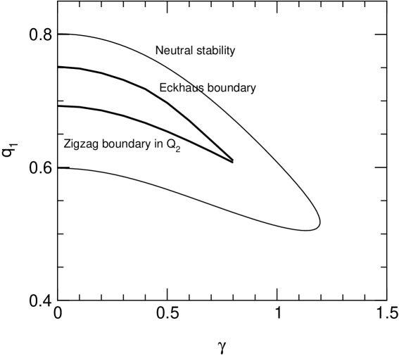
Figure 2: Neutral stability curve and secondary instability boundaries for an initially transverse lamella with $\omega=0.01$ and $\epsilon=0.04$.

First consider initially transverse lamellae, i.e., with ${\bf q}$ along the $x_{1}$ direction. From Fig. 1 it is clear that the shear flow will tilt the layers, and in doing so decrease their wavelength. The stability diagram for this case has been obtained by numerical solution of the Floquet problem for $\omega=0.01$ and $\epsilon=0.04$ and is shown in Fig. 2 as a function of the shear amplitude $\gamma$. The outside bounding curves are the neutral stability boundaries so that only within this range a nonlinear solution for $\psi$ exists, with an amplitude $A(t)$ given by Eq. (9). The bending of the curves toward smaller values of $q$ as $\gamma$ increases can be qualitatively understood by noting that the oscillatory shear leads to a decrease in the lamellar wavelength. Thus at higher values of $\gamma$, the region of existence of finite amplitude solutions shifts toward larger wavelengths to compensate for a larger reduction in wavelength by the flow. At large enough $\gamma$, however, nonlinear solutions cease to exist.

Only nonlinear solutions within the inner region in Fig. 2 are stable against long wavelength secondary instabilities. Both Eckhaus and zig-zag type instabilities occur as shown in the figure. The Eckhaus instability is a longitudinal phase instability (${\bf Q}\parallel{\bf q}$) so that through coupling with the amplitude it leads to an amplitude modulation in the same direction as the base periodicity. In general, this instability appears in the large wavenumber range of the diagram and is qualitatively interpreted as an instability that leads to a decrease in the wavenumber by eliminating lamellar layers through the amplitude modulation. On the other hand, in the range of small $q$, a zig-zag instability with ${\bf Q}\perp{\bf q}$ can lead to an increase in $q$ to return the unstable lamella to the stable range. In the absence of shear, perturbations to a base state defined by ${\bf q}=q\hat{\bf x}_{1}$ along $Q\hat{\bf x}_{2}$ or $Q\hat{\bf x}_{3}$ are equivalent. Under shear, however, the degeneracy is broken, and we find from the numerical Floquet analysis that the marginal mode for the zig-zag instability is $Q\hat{\bf x}_{2}$, i.e., along the perpendicular direction. In summary, the large wavenumber instability is of the Eckhaus type and does not lead to lamellar reorientation. The small wavenumber instability is of zig-zag type, and leads to a growing component along the perpendicular direction.

We next turn to a geometrical interpretation of these results based on a rigid distortion of the lamellar structure as discussed above. The marginal wavevector for an unstable zigzag perturbation can be either ${\bf q}+{\bf Q}=(q,Q,0)$ which leads to growth of a perpendicular component, or ${\bf q}+{\bf Q}=(q,0,Q)$ that leads to a parallel orientation. The effective wavenumber of the distortion in each case is given by

$$\hbox{perpendicular zigzag}\quad|{\mathbf{q}}+{\mathbf{Q}}|^{2}(t) = |(q,Q,\tilde{\gamma}q)|^{2}=(1+\tilde{\gamma}^{2})q^{2}+Q^{2}$$

$$\hbox{parallel zigzag}\quad|{\mathbf{q}}+{\mathbf{Q}}|^{2}(t) = |(q,0,\tilde{\gamma}q+Q)|^{2}=(1+\tilde{\gamma}^{2})q^{2}+2\tilde{\gamma}qQ+Q^{2}.$$

Under oscillatory shear $\tilde{\gamma}$ changes sign and both cases lead to a wavenumber increase, although given the sign change, it is not possible to tell which mode is more effective at increasing the wavenumber following the instability. This is the only case in which this geometric interpretation does not lead to a selected marginal mode consistent with the Floquet analysis. We note, however, that if the shear were stationary instead $\tilde{\gamma}$ increases monotonically, and a zig-zag instability along the parallel direction would provide for a larger increase in wavenumber.

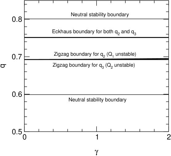
Figure 3: Neutral stability curve and secondary instability boundaries for initially parallel and perpendicular lamellae with $\omega=0.01$ and $\epsilon=0.04$.

We now consider a base lamellar phase oriented parallel to the shear. Figure 3 shows the stability boundaries computed numerically. As seen in the figure, secondary instabilities are again of the Eckhaus type at large $q$, and of zig-zag type at small $q$. In this case the location of the boundary is nearly independent of $\gamma$, i.e., the shear flow has no effect on the Eckhaus instability. This can be understood geometrically from Fig. 1 since the parallel orientation is unaffected by the shear, and an Eckhaus instability of a parallel orientation would also lead to a growing mode along the parallel orientation. The zig-zag boundary at small wavenumbers also remains constant and unaffected by the shear. Nevertheless shear flow does introduce a distinction between the two possible zig-zag modes along the perpendicular and transverse directions respectively. The former, given by ${\bf q}=(0,Q,q)$, will not be advected by the shear according to the Eq. (19). The latter is given by ${\bf q}=(Q,0,q)$, and it has its wavenumber advected as $q(t)=(q-\tilde{\gamma}Q)^{2}+Q^{2}$. Therefore the shear leads to a net wavenumber increase only when the instability is along the transverse direction. The results of the Floquet analysis are consistent in this case with the orientation that produces the largest wavenumber increase.

We finally discuss the case of initially perpendicular lamellae. The stability boundaries for this case are also shown in Fig. 3. Again, the Eckhaus boundary is unaffected by the shear. This can be understood from Fig. 1 since the perpendicular orientation does not couple to the flow. An Eckhaus mode is along the perpendicular direction as well, and hence remains unaffected by the shear. On the other hand there is a very weak dependence of the zig-zag stability boundary on the shear amplitude, and we find that the marginal mode is along the transverse direction. This is also consistent with the geometric interpretation given earlier since an imposed shear flow will always increase the wavenumber for a transverse zig-zag mode $(Q,q,0)$, but has no effect on a parallel zig-zag mode $(0,q,Q)$:

$$\hbox{transverse zigzag}\quad|{\mathbf{q}}+{\mathbf{Q}}|^{2}(t) = |(Q,q,\gamma Q)|^{2}=q^{2}+(1+\gamma^{2})Q^{2}$$

$$\hbox{parallel zigzag}\quad|{\mathbf{q}}+{\mathbf{Q}}|^{2}(t) = |(0,q,Q)|^{2}=q^{2}+Q^{2}$$

Our results for the the secondary instabilities of the three particular lamellar orientations can be classified according to the orientation of the marginal mode as follows:

$$\begin{array}[]{lcl}\hbox{Transverse lamellae}&\rightarrow&\hbox{zig-zag to perpendicular orientation}\\ \hbox{Parallel lamellae}&\rightarrow&\hbox{zig-zag to perpendicular orientation}\\ \hbox{Perpendicular lamellae}&\rightarrow&\hbox{zig-zag to transverse orientation}\end{array}$$

If one assumes that the orientation of the marginal mode sets a preference for the final orientation of the emerging stable lamellar structure, our results suggest that the perpendicular alignment is the preferred orientation under the action of the oscillatory shear, independently of viscosity contrast (within the Newtonian viscosity model adopted). Even in the case in which an instability of a perpendicular orientation leads to a transverse state, a shear flow of small amplitude would drive it back to the perpendicular orientation, presumably now with a wavenumber inside the stable region. We however need to be remain cautious about the generality of this conclusion as a complex dynamical evolution could follow the initial decay after a zig-zag instability. For example, our earlier numerical results in ref. [15] showed that a zig-zag instability may lead to kink-band formation, and yet to another orientation change as the bands themselves become unstable.

We finally present the stability diagram in full three dimensional ${\bf q}$ space for a base lamellar state of arbitrary orientation relative to the shear. In the absence of flow, all lamellae with wavenumbers near the marginal value $q_{c}$ are stable. Hence the stability region is a spherical shell in ${\bf q}$ space. Under shear, any lamella with a wavevector that has a significant component along the transverse direction becomes unstable, and the region of stability becomes compressed along the $q_{1}$ direction. For sufficiently large $\gamma$, the stable region adopts a toroidal shape around the $q_{2}$–$q_{3}$ plane with a small projection in the $q_{1}$ direction that depends on $\gamma$. Although we have argued earlier that lamellae with a too small wavenumber will become unstable to a zig-zag mode and evolve into a new state oriented along the perpendicular direction, this by no means implies that a stable parallel orientation cannot exist (although perhaps within a narrow range of wavenumbers).

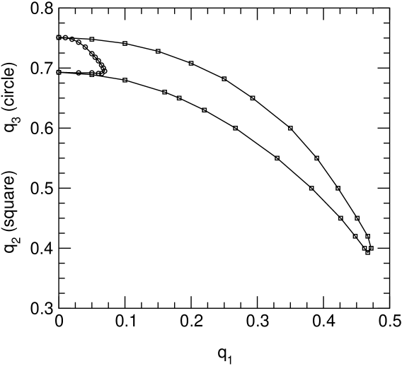
Figure 4: Stability regions in the $q_{1}$–$q_{2}$ and $q_{1}$–$q_{3}$ planes with $\omega=0.01$, $\gamma=1$, and $\epsilon=0.04$.

As an example, Fig. 4 shows the complete stability boundaries along both $q_{2}$–$q_{1}$ and $q_{3}$–$q_{1}$ planes for $\epsilon=0.04$ and $\gamma=1$. Note how the stable region in the $q_{2}$–$q_{1}$ plane is significantly larger than in the $q_{3}$–$q_{1}$ plane. This is also evidenced in Fig. 5 by the asymmetry in the toroidal stability region which is wide near the $q_{2}$ axis (the perpendicular direction) but narrow near the $q_{2}$ direction (the parallel axis). The implication of this result is that if an initially disordered state is comprised of many domains locally oriented along arbitrary directions, one would expect that a larger portion of the sample would remain in the perpendicular state, as it corresponds to the one with the largest region of stability in ${\bf q}$ space. This argument is distinct from that given above involving the orientation of the marginal model following a secondary instability of a perfectly ordered lamellar structure, but it suggests the same dominant orientation.

In addition to the detailed numerical computation of the stability region in ${\bf q}$ space, the relative sizes of the stability regions for parallel and perpendicular orientations may be estimated from the geometric interpretation given above. Consider first an almost perpendicular state with a wavevector of a magnitude $q_{0}$ with a small component $\Delta q$ in the transverse direction. Under the action of the shear, Eq. (19) gives for the time dependent wavenumber

$$q(t)=\left[\Delta q^{2}+q_{0}^{2}+(\tilde{\gamma}\Delta q)^{2}\right]^{\frac{1}{2}}\approx q_{0}\left[1+\frac{1}{2}(1+\tilde{\gamma}^{2})\left(\frac{\Delta q}{q_{0}}\right)^{2}\right].$$

Therefore the wavenumber increases with the shear as $(\Delta q/q_{0})^{2}$. On the other hand, an almost parallel state has a wavenumber

$$q(t)=\left[\Delta q^{2}+(\tilde{\gamma}\Delta q+q_{0})^{2}\right]^{\frac{1}{2}}\approx q_{0}\left(1+\tilde{\gamma}\frac{\Delta q}{q_{0}}\right),$$

and therefore it increases only linearly with $\Delta q/q_{0}$. These two relations essentially yield the dependence of the width of the toroidal region in Fig. 5 along the transverse direction, and therefore the fact that the relative extent of the perpendicular region of stability is larger than the parallel region.

Insofar our results could be used to infer the dominant orientation under shear, our conclusions would differ from those of Fredrickson [7], from low frequency experimental evidence in PEP-PEE, but agree with some low frequency experimental evidence in PS-PI. One must caution, however, that as discussed in ref. [7], it is not clear which of the two systems PEP-PEE or PS-PI has a larger value of $\eta_{1}$, or how close they are to the assumed Newtonian behavior. Therefore we must consider our results to be a baseline against which to compare future work involving true viscoelastic contrast between the microphases.

Finally it is interesting to address a possible reason for the qualitative discrepancy between the conclusions of our work and those of Fredrickson’s concerning the effect of viscosity contrast. Although he discussed the case of steady shear, our results are confined to low frequencies, and are only weakly dependent on frequency. Therefore the discrepancy in conclusions is not likely to arise from the time dependence of our solutions. Briefly, he found a transition from a high temperature disordered state to parallel lamellae at low shear rates, and to perpendicular lamellar at high shear rates. In the latter case, and upon further decrease in temperature, he predicted another transition to a parallel state. The location of this second transition line depended on the viscosity contrast between the microphases. Instead, we see no discernible effect arising from viscosity contrast. A possible qualitative explanation can be given as follows: Our calculation is conducted at an externally imposed shear rate $D=v_{p}/d$ in dimensional units (here and in what follows), where $v_{p}$ is the velocity of the solid boundary. Consider a parallel configuration comprised of only two planar layers with uniform shear viscosity $\eta_{0}+\eta_{1}$ and $\eta_{0}-\eta_{1}$ respectively. The average shear rate of this configuration is given by

$$\langle D\rangle=\frac{1}{d}\left[\frac{d}{2}\frac{(v^{\prime}-0)}{d/2}+\frac{d}{2}\frac{(v_{p}-v^{\prime})}{d/2}\right]=D,$$

where $v^{\prime}$ is the (unknown) speed at the boundary between the two layers. In this case, the average shear rate is independent of the viscosity contrast. On the other hand and following Fredrickson, if the boundary conditions involve an imposed shear stress $\sigma$, the conclusion is different. The shear rate for the base state is now $D=\sigma/\eta_{0}$, the same as in the previous case. However, in the creeping flow approximation considered, the shear stress is uniform in the fluid, but the shear rate is different in the two layers,

$$D_{1}(\eta_{0}-\eta_{1})=D_{2}(\eta_{0}+\eta_{1})=D\eta_{0},$$

where $D_{1}$ (resp. $D_{2}$) is the shear rate in the layer of viscosity $\eta_{0}-\eta_{1}$ (resp. $\eta_{0}+\eta_{1}$). The spatial average over the configuration is now,

$$\langle D\rangle=\frac{1}{d}\left[\frac{d}{2}D_{1}+\frac{d}{2}D_{2}\right]=\frac{D}{2}\left(\frac{1}{1-\delta}+\frac{1}{1+\delta}\right)=D\left(1+\delta^{2}+\ldots\right),$$

where $\delta=\eta_{1}/\eta_{0}$. Therefore the average shear rate across the layer in a parallel configuration always increases with viscosity contrast. (In both sets of calculations, the perpendicular base state is not affected by the shear flow). Fredrickson’s results are based on the introduction of a renormalized order parameter mobility that is assumed to depend on the average shear rate across the layer. Therefore his results for a parallel configuration are affected by the shear, whereas ours are not. As discussed in Section 3, the composition field of the base parallel configuration is not modified by the flow correction arising from viscosity contrast. Finally, although the implications of the choice of boundary conditions on the dynamical evolution of partially ordered lamellar configurations are difficult to establish, we note that Fredrickson’s work focused on fluctuations near a uniform, disordered state, whereas we have considered perturbations around a (weakly) nonlinear state of a finite amplitude, saturated lamellar structure.

Figure 5: Region of stability of a uniform lamella as a function of its orientation. The axes correspond to transverse ($q_{1}$), perpendicular ($q_{2}$), and parallel ($q_{3}$) orientations. The surface has been determined by numerical solution of the Floquet problem defined by Eq. (18) with $\omega=0.01$, $\gamma=1$, and $\epsilon=0.04$

References

- [1] Bates, F.; Fredrickson, G. Annu. Rev. Phys. Chem. 1990, 41, 525.
- [2] Hamley, I. The Physics of Block Copolymers; Oxford University Press: New York, 1998.
- [3] Fredrickson, G.; Bates, F. Annu. Rev. Mater. Sci. 1996, 26, 501.
- [4] Hadziiaannou, G.; Mathis, A.; Skoulios, A. Colloid Polym. Sci. 1979, 257, 136.
- [5] Koppi, K.; Tirrell, M.; Bates, F.; Almdal, K.; Colby, R. J. Phys. II (France) 1992, 2, 1941.
- [6] Koppi, K.; Tirrel, M.; Bates, F. Phys. Rev. Lett. 1993, 70, 1449.
- [7] Fredrickson, G. J. Rheol 1994, 38, 1045.
- [8] Patel, S.; Larson, R.; Winey, K.; Watanabe, H. Macromolecules 1995, 28, 4313.
- [9] Gupta, V.; Krishnamoorti, R.; Kornfield, J.; Smith, S. Macromolecules 1995, 28, 4464.
- [10] Maring, D.; Wiesner, U. Macromolecules 1997, 30, 660.
- [11] Leist, H.; Maring, D.; Thurn-Albrecht, T.; Wiesner, U. J. Chem. Phys. 1999, 110, 8225.
- [12] Tepe, T.; Hajduk, D.; Hillmyer, M.; Weimann, P.; Tirrell, M.; Bates, F. J. Rheol. 1997, 41, 1147.
- [13] Kodama, H.; Doi, M. Macromolecules 1996, 29, 2652.
- [14] Shiwa, Y. Physics Letters A 1997, 228, 279.
- [15] Drolet, F.; Chen, P.; Viñals, J. Macromolecules 1999, 32, 8603.
- [16] Leibler, L. Macromolecules 1980, 13, 1602.
- [17] Ohta, T.; Kawasaki, K. Macromolecules 1986, 19, 2621.
- [18] Oono, Y.; Bahiana, M. Phys. Rev. Lett. 1988, 61, 1109.
- [19] Gurtin, M. E.; Polignone, D.; Viñals, J. Math. Models and Methods in Appl. Sci. 1996, 6, 815.
- [20] Polis, D.; Winey, K.; Ryan, A.; Smith, S. Phys. Rev. Lett. 1999, 83, 2861.
- [21] The nonlinear saturation of this perturbation will not be addressed, and therefore we do need to consider the relative magnitude of the two small parameters: and the amplitude of the long wavevelength perturbation.
- [22] Cross, M.; Hohenberg, P. Rev. Mod. Phys. 1993, 65, 851.