Universal Features of Interacting Chaotic Quantum Dots.
Application to Statistics of Coulomb Blockade Peak Spacings.

Abstract

We present a complete classification of the electron-electron interaction in chaotic quantum dots based on expansion in inverse powers of $1/M$, the number of the electron states in the Thouless window, $M\simeq k_{F}R$. This classification is quite universal and extends and enlarges the universal non interacting RMT statistical ensembles. We show that existing Coulomb blockade peak spacing data for $B=0$ and $B\neq 0$ is described quite accurately by the interacting GSE and by its extension to $B\neq 0$. The bimodal structure existing in the interacting GUE case is completely washed out by the combined effect of the spin orbit, pairing and higher order residual interactions.

Measurement of the fluctuations of the Coulomb blockade (CB) peak spacings as well as the mesoscopic spin effects provide an excellent probe of the properties of interaction effects in disordered quantum dots (QD). Basic experiments where performed [1, 2] in ballistic, well isolated QD of irregular shape formed in $2d$ GaAs heterostructures. The QD sizes were $R\gg 1/k_{F}$, where $k_{F}$ is the electron Fermi wave vector.

The main general theme underlying this problem is an interplay between chaos and interactions in quantum mechanical motion of electrons in a restricted geometry. In a recent work [3], cf., also [4], on mesoscopic spin effects a proposal appeared for a universal Hamiltonian which controls the main physics of interactions in a chaotic QD in the extreme limit $k_{F}R\gg 1$. In [5] statistical fluctuations around this limit were included in the framework of the Hartree-Fock (HF) method. Our main goal here is to show that these fluctuations and indeed the entire interacting Hamiltonian can be represented and classified in a unifying  universal scheme, cf. Eqs. (11,15,19) below, which follows and extends the universal symmetry classes of the Wigner-Dyson statistical theory for non interacting electrons. Our second goal is to apply this theory to the problem of fluctuations of the CB peak spacings. Although this has received much attention recently [6, 7, 8, 9, 5], a consistent description is still lacking. We will show that the universal interacting GSE Hamiltonian and its extension (we call it GUSE) to the non zero magnetic field in our scheme accounts quite well for the experimental distributions, cf. Fig. 1 below. The GSE choice matches perfectly the recently discovered strong spin-orbit (SO) effects in GaAs QD, [4]

The Hamiltonian of an interacting QD consists of one and two body parts, $H=H_{0}+H_{int}$.

$$H_{0}=\sum_{a,b,\sigma,\sigma^{\prime}}H_{a\sigma,b\sigma^{\prime}}a_{a\sigma}^{\dagger}a_{b\sigma^{\prime}}=\sum_{\alpha\nu}\epsilon_{\alpha}a_{\alpha\nu}^{\dagger}a_{\alpha\nu},$$ (1)

$$H_{int}=\frac{1}{2}\sum V_{\alpha\nu_{1},\beta\nu_{2};\gamma\nu_{3},\delta\nu_{4}}a_{\alpha\nu_{1}}^{\dagger}a_{\beta\nu_{2}}^{\dagger}a_{\delta\nu_{4}}a_{\gamma\nu_{3}},$$ (2)

Here indices $a,b$ denote space orbitals while $\sigma,\sigma^{\prime}$ are the spin indices. With a possible SO interaction $H_{a\sigma,b\sigma^{\prime}}$ is in general not diagonal in the spin indices. We use $\alpha,\nu$ to numerate the eigen states of $H_{a\sigma,b\sigma^{\prime}}$; $\epsilon_{\alpha}$ are its eigen energies with $\alpha$ the orbital and $\nu=\pm\frac{1}{2}$ - the spin or Kramers index in the presence of SO. In irregular QD the one electron Hamiltonian in the Thouless window of states can be described by a random matrix theory (RMT),[10, 11, 12]. We will denote by $M$ the rank of $H_{a\sigma,b\sigma^{\prime}}$. The statistics of $H_{a\sigma,b\sigma^{\prime}}$ depends on the symmetry of the problem classified by standard RMT ensembles - GOE, GUE and GSE. The correlators of the eigen functions of $H_{a\sigma,b\sigma^{\prime}}$ depend on the ensemble. For GOE they are

$$<\psi_{\alpha\nu}^{\ast}({\bf r,\sigma})\psi_{\beta\nu^{\prime}}({\bf r}^{\prime},\sigma^{\prime})>=<\psi_{\alpha\nu}({\bf r,\sigma})\psi_{\beta\nu^{\prime}}({\bf r}^{\prime},\sigma^{\prime})>$$ (3)

$$=<\psi_{\alpha\nu}^{\ast}({\bf r,\sigma})\psi_{\beta\nu^{\prime}}^{\ast}({\bf r}^{\prime},\sigma^{\prime})>=\delta_{\nu\sigma}\delta_{\nu^{\prime}\sigma^{\prime}}\delta_{\alpha\beta}K({\bf r},{\bf r}^{\prime}).$$ (4)

We find it convenient to work in the coordinate-spin representation (${\bf r},\sigma)$. The function $K({\bf r},{\bf r}^{\prime})$ is

$$K({\bf r},{\bf r}^{\prime})=\frac{1}{2M}\sum_{\alpha=1}^{M}\sum_{\nu\sigma}\psi_{\alpha\nu}^{\ast}({\bf r,\sigma})\psi_{\alpha\nu}({\bf r}^{\prime},\sigma)$$ (5)

$$\simeq A^{-1}J_{0}(k_{F}|{\bf r}-{\bf r}^{\prime}|).$$ (6)

Here $A$ is the area of QD and $J_{0}(x)$ is the zero order Bessel function giving an approximate quasiclassical expression for $K({\bf r},{\bf r}^{\prime})$, [13]. For the GUE the correlators of the type $<\psi\psi>$, and $<\psi^{\ast}\psi^{\ast}>$ are zero while $<\psi^{\ast}\psi>$ is the same as in GOE. For the GSE symmetry one has

$$< \psi_{\alpha\nu}^{\ast}({\bf r,\sigma})\psi_{\beta\nu^{\prime}}({\bf r}^{\prime},\sigma^{\prime})>=\frac{1}{2}\delta_{\nu\nu^{\prime}}\delta_{\sigma\sigma^{\prime}}\delta_{\alpha\beta}K({\bf r},{\bf r}^{\prime}),$$ (7)

$$< \psi_{\alpha\nu}({\bf r,\sigma})\psi_{\beta\nu^{\prime}}({\bf r}^{\prime},\sigma^{\prime})>=\frac{1}{2}k_{\nu\nu^{\prime}}k_{\sigma\sigma^{\prime}}\delta_{\alpha\beta}K({\bf r},{\bf r}^{\prime}),$$ (8)

$\hat{k}$ is $2\times 2$ time inversion matrix for spin $\frac{1}{2}$ systems [10].

It is convenient to consider the interaction part of the Hamiltonian $H_{int}$ in the basis of the eigen functions $\psi_{\alpha\nu}$ of the one electron Hamiltonian

$$V_{\alpha\nu_{1},\beta\nu_{2};\gamma\nu_{3},\delta\nu_{4}}=V^{*}_{\gamma\nu_{3},\delta\nu_{4};\alpha\nu_{1},\beta\nu_{2}}=\int d{\bf r}d{\bf r}^{\prime}\times$$ (9)

$$\psi_{\alpha\nu_{1}}^{\ast}({\bf r},\sigma)\psi_{\beta\nu_{2}}^{\ast}({\bf r}^{\prime},\sigma^{\prime})U({\bf r},{\bf r}^{\prime})\psi_{\gamma\nu_{3}}({\bf r},\sigma)\psi_{\delta\nu_{4}}({\bf r}^{\prime},\sigma^{\prime}).$$ (10)

Here $U({\bf r},{\bf r}^{\prime})$ is the the screened electron - electron interaction in QD. If SO interaction is absent the space and spin coordinates ${\bf r}$ and $\sigma$ are separated.

It is possible to represent the interaction (9) as a sum of parts of different order in a small parameter $1/M$. An essential step in this direction was made in [3]. Here we shall present the complete classification and investigate some of its consequences. We will only present our main results deferring the detailed derivations to Ref. [15]. It will be sufficient here to assume that higher correlators of $\psi$’s obey the rules of the Gaussian statistics. The role of the non Gaussian corrections will be discussed in [15]. We use a cluster decomposition of the matrix elements (9) as fourth order polynomial functions of the random wave functions $\psi$. Inserting this into $H_{int}$ we find that it consists of three groups of terms $H_{int}=H_{int}^{(0)}+H_{int}^{(1)}+H_{int}^{(2)}$. For the GOE these terms are

$$H_{int}^{(0)}=\frac{1}{2}V_{c}\hat{N}(\hat{N}-1)-J\hat{{\bf S}}^{2}+P\hat{T}^{\dagger}\hat{T},$$ (11)

$$H_{int}^{(1)}=\hat{N}\sum_{\alpha\beta}u_{\alpha\beta}^{n}(a_{\alpha}^{\dagger}\cdot a_{\beta})+\hat{{\bf S}}\cdot\sum_{\alpha\beta}u_{\alpha\beta}^{s}(a_{\alpha}^{\dagger}\mbox{\boldmath{$\sigma$}}a_{\beta})+$$ (12)

$$+\hat{T}^{\dagger}\sum_{\alpha\beta}u_{\alpha\beta}^{p}a_{\alpha\downarrow}a_{\beta\uparrow}-\sum_{\alpha\beta}u_{\alpha\beta}^{p\ast}a_{\alpha\downarrow}^{\dagger}a_{\beta\uparrow}^{\dagger}\hat{T},$$ (13)

$$H_{int}^{(2)}=\frac{1}{2}\sum_{\alpha\beta\gamma\delta\sigma\sigma^{\prime}}\tilde{V}_{\alpha\beta;\gamma\delta}a_{\alpha\sigma}^{\dagger}a_{\beta\sigma^{\prime}}^{\dagger}a_{\delta\sigma^{\prime}}a_{\gamma\sigma}.$$ (14)

Here we denoted by dot the scalar product in the spin variables, $\hat{N}=\sum_{\alpha}(a_{\alpha}^{\dagger}\cdot a_{\alpha})$ is the operator of the total number of electrons, $\hat{{\bf S}}=\frac{1}{2}\sum_{\alpha}(a_{\alpha}^{\dagger}\mbox{\boldmath{$\sigma$}}a_{\alpha})$ is the operator of the total spin, $\sigma$ are the Pauli matrices and $\hat{T}=\sum_{\alpha}a_{\alpha\downarrow}a_{\alpha\uparrow}$ is the total pairing operator. The decomposition (11) is an identity which is useful since as we will show below and in [15] it allows to classify the groups of terms $H_{int}^{(0)}$, $H_{int}^{(1)}$ and $H_{int}^{(2)}$ by their degree of smallness with respect to $1/M.$ Namely, apart of the capacitance term $V_{c}\sim M\Delta$ ($\Delta$ is mean level spacing) and up to logarithmic corrections the matrix elements in $H_{int}^{(n)}$ are $\sim\Delta/(M)^{n/2}.$ The properties of $u$ and $\tilde{V}$ are discussed below,cf. also Ref. [6, 5].

For GUE the expression above remains valid except that the terms containing the pairing operators $T$ and $T^{\dagger}$ are absent. For GSE the expression (11) becomes

$$H_{int}^{(0)}=\frac{1}{2}V_{c}\hat{N}(\hat{N}-1)+P\hat{T}^{\dagger}\hat{T},$$ (15)

$$H_{int}^{(1)}=\hat{N}\sum_{\alpha\nu\beta\nu^{\prime}}u_{\alpha\nu\beta\nu^{\prime}}^{n}a_{\alpha\nu}^{\dagger}a_{\beta\nu^{\prime}}+$$ (16)

$$+\hat{T}^{\dagger}\sum_{\alpha\nu\beta\nu^{\prime}}u_{\alpha\nu\beta\nu^{\prime}}^{p}a_{\alpha\nu}a_{\beta\nu^{\prime}}-\sum_{\alpha\nu\beta\nu^{\prime}}u_{\alpha\nu\beta\nu^{\prime}}^{p\ast}a_{\alpha\nu}^{\dagger}a_{\beta\nu^{\prime}}^{\dagger}\hat{T},$$ (17)

$$H_{int}^{(2)}=\frac{1}{2}\sum_{\alpha\nu_{1}\beta\nu_{2}\gamma\nu_{3}\delta\nu_{4}}\tilde{V}_{\alpha\nu_{1}\beta\nu_{2};\gamma\nu_{3}\delta\nu_{4}}a_{\alpha\nu_{1}}^{\dagger}a_{\beta\nu_{2}}^{\dagger}a_{\delta\nu_{4}}a_{\gamma\nu_{3}}.$$ (18)

Now the terms containing the spin operators disappear and the spin index is replaced by the Kramers degeneracy index which we denote by $\nu$. The matrices $u^{n,p}$ and $\tilde{V}$ depend on $\nu$.

Introduction of a perpendicular magnetic field removes the Kramers degeneracy and changes the statistics of the single particle Hamiltonian into GUE(2M). But this is not the interacting GUE obtained from (11). The second correlator in (7) vanishes and consequently the terms containing the pairing operators $T$, $T^{\dagger}$ in (15) disappear. Also there is no need anymore for the Kramers spinor indices in $u^{n}$ and $\tilde{V}$. Thus one obtains a different 1/M expansion which we term GUSE (unitary arising from simplectic)

$$H_{int}^{(GUSE)}=\frac{1}{2}V_{c}\hat{N}(\hat{N}-1)+\hat{N}\sum_{\alpha,\beta=1}^{2M}u_{\alpha\beta}^{n}a_{\alpha}^{\dagger}a_{\beta}+$$ (19)

$$+\frac{1}{2}\sum_{\alpha,\beta,\gamma,\delta=1}^{2M}\tilde{V}_{\alpha\beta;\gamma\delta}a_{\alpha}^{\dagger}a_{\beta}^{\dagger}a_{\delta}a_{\gamma}.$$ (20)

Such an ensemble was first discussed in [4].

The lowest order $H_{int}^{(0)}$ in (11) and its universality was fully discussed in [3]. The $\frac{1}{2}V_{c}\hat{N}(\hat{N}-1)$ term is at the basis of the simplest Coulomb blockade theory while $J\hat{{\bf S}}^{2}$ appeared in relation to mesoscopic spin fluctuations, [4]. Here we will discuss higher order terms and will then explore their effect and interplay with the $T^{\dagger}T$ term. We note, [15], that $u$ and $\tilde{V}$ are such that $<u_{\alpha\beta}^{i}>$=
$<\tilde{V}_{\alpha\beta\gamma\delta}>=0$ for $i=n,s,p$, and the average of the second functional derivatives of $\tilde{V}$ with respect to $\psi$ or $\psi^{\ast}$ is equal to zero. Up to corrections of the order $1/M$ the matrices $u_{\alpha\beta}^{i},\ u_{\alpha\nu\beta\nu^{\prime}}^{i}$ for $i=n,s,p$, are Gaussian random variables with zero average. For GOE one finds, [5, 15] ,

$$<u_{\alpha\beta}^{i\ast}u_{\alpha^{\prime}\beta^{\prime}}^{i^{\prime}}>=$$ (21)

$$=C_{ii^{\prime}}\frac{\Delta^{2}}{M}\left(\delta_{\alpha\alpha^{\prime}}\delta_{\beta\beta^{\prime}}+\delta_{\alpha\beta^{\prime}}\delta_{\beta\alpha^{\prime}}-\frac{2}{M}\delta_{\alpha\beta}\delta_{\alpha^{\prime}\beta^{\prime}}\right).$$ (22)

Here $C_{ii^{\prime}}=C_{i^{\prime}i}$ are 6 dimensionless constants which depend on the average geometry of as well as on the details of the electron screening in QD (cf., below). On the basis of the correlators (7) one can find similar averages for GUE, GSE and GUSE. For GUE the correlators of the residual interaction $\tilde{V}$ in (15) are, [5, 15]

$$<\tilde{V}_{\alpha\beta;\gamma\delta}^{\ast}\tilde{V}_{\alpha^{\prime}\beta^{\prime};\gamma^{\prime}\delta^{\prime}}>=\frac{\Delta^{2}\ln M}{M^{2}}\times$$ (23)

$$\times D\{\delta_{\alpha\alpha^{\prime}}\delta_{\beta\beta^{\prime}}\delta_{\gamma\gamma^{\prime}}\delta_{\delta\delta^{\prime}}+\delta_{\alpha\beta^{\prime}}\delta_{\beta\alpha^{\prime}}\delta_{\gamma\delta^{\prime}}\delta_{\delta\gamma^{\prime}}+$$ (24)

$$+\delta_{\alpha\alpha^{\prime}}\delta_{\beta\beta^{\prime}}\delta_{\gamma\delta^{\prime}}\delta_{\delta\gamma^{\prime}}+\delta_{\alpha\beta^{\prime}}\delta_{\beta\alpha^{\prime}}\delta_{\gamma\gamma^{\prime}}\delta_{\delta\delta^{\prime}}\}+O(M^{-2})$$ (25)

where $D$ is again a dimensionless largely universal constant (cf., below). One can easily write corresponding expressions for other ensembles.

In order to proceed it is convenient to adopt the following decomposition of the basic screened e-e interaction $U({\bf r},{\bf r})$ in (9), cf., [6]

$$U({\bf r},{\bf r}^{\prime})=V_{c}+u^{sur}({\bf r})+u^{sur}({\bf r}^{\prime})+V({\bf r},{\bf r}^{\prime}).$$ (26)

Here $V_{c}$ is the constant capacitance part, cf., (11,15), $u^{sur}({\bf r})$ is the surface part of the potential caused by the screening charges which are on the surface and $V({\bf r},{\bf r}^{\prime})$ is the screened bulk e-e interaction. One can express the constants entering in the expressions (11,15,19) in terms of $u^{sur}({\bf r})$ and $V({\bf r},{\bf r}^{\prime})$. For GOE one finds (expressions for other ensembles are very similar), [15]

$$J=P=I_{2},\ \ I_{n}=A^{n-2}\int K^{n}({\bf r},{\bf r}^{\prime})V({\bf r},{\bf r}^{\prime})d{\bf r}d{\bf r}^{\prime};$$ (27)

$$u_{\alpha\beta}^{i}=\int u^{i}({\bf r},{\bf r}^{\prime})\psi_{\alpha}^{\ast}({\bf r})\psi_{\beta}({\bf r^{\prime}})d{\bf r}d{\bf r}^{\prime},i=n,s,p;$$ (28)

Here $u^{n}({\bf r},{\bf r}^{\prime})=\delta({\bf r}-{\bf r}^{\prime})(u^{sur}({\bf r})-\bar{u})-(1/2)u^{s}({\bf r},{\bf r}^{\prime})$, $\ u^{p}({\bf r},{\bf r}^{\prime})=u^{s}({\bf r},{\bf r}^{\prime})$ , $\bar{u}=A^{-1}\int u^{sur}({\bf r})d{\bf r}$ and $u^{s}({\bf r},{\bf r}^{\prime})=K({\bf r},{\bf r}^{\prime})V({\bf r},{\bf r}^{\prime})-J\delta({\bf r}-{\bf r}^{\prime}).$ The matrix $\tilde{V}_{\alpha\beta;\gamma\delta}$ is given by (9) if we substitute $U({\bf r},{\bf r}^{\prime})\Rightarrow V({\bf r},{\bf r}^{\prime})$ and extract the irreducible part. We also have

$$C_{ii^{\prime}}=\frac{M}{\Delta^{2}}\int K(1,3)K(2,4)u^{i}(1,2)u^{i^{\prime}}(3,4)d\Omega,$$ (29)

$$D=\frac{M^{2}}{\Delta^{2}\ln M}\int K^{2}(1,3)K^{2}(2,4)V(1,2)V(3,4)d\Omega,$$ (30)

where $V(1,2)\equiv V({\bf r}_{1},{\bf r}_{2})$, etc., and $d\Omega\equiv d{\bf r}_{1}d{\bf r}_{2}d{\bf r}_{3}d{\bf r}_{4}$.

We now turn to the problem of the fluctuations of the spacings between Coulomb blockade peaks. We focus on the experiments in 2D GaAs dots, Ref. [1]. An important observation made in [4] was that the basic non interacting Hamiltonian for such dots must include a strong SO interaction, the so called Rashba term [14], $\alpha_{SO}\hat{{\bf p}}\cdot[\hat{{\bf s}}\times{\bf n}],$ where $\hat{\bf p}$ and $\hat{\bf s}$ are the momentum and spin operators, ${\bf n}$ is the vector of the normal to the QD plane. The strength of this term in a typical GaAs/GaAlAs heterostructure is $\alpha_{SO}\simeq 2.5\cdot 10^{-7}mev\ cm/\hbar$ [14]. The corresponding energy scale $\sim 0.3$ mev is $\gg\Delta$. Thus it is appropriate to use the GSE ensemble for the random single electron Hamiltonian and the expression (15) for the interaction. The pairing term $T^{\dagger}T$ unlike other zeroth order terms does not commute with the random single electron part and should therefore increase the effect of fluctuations. Experiments in [1] included also the situation with an applied weak perpendicular magnetic field. This corresponds to the GUSE Eq. (19).

For the QD parameters we use $\Delta=2\hbar^{2}/(m^{\ast}R^{2})$, $E_{F}=\pi\hbar^{2}/(m^{\ast}r_{sc}^{2})$, $r_{sc}\simeq n_{c}^{-1/2}$, where $m^{\ast}$ is the effective mass, $n_{c}$ is the electron concentration in a QD. The Thouless energy is $E_{Th}=\hbar/\tau_{bal}=\sqrt{2\pi}\hbar^{2}/(m^{\ast}r_{sc}R)$. From Eq. (5) it follows that the rank of RMT is $M\simeq\pi Rk_{F}/2$ so that $M\simeq\pi^{3/2}R/(2r_{sc})$. The constants in the interacting part of the GSE Hamiltonian (15) are completely determined by $u^{sur}({\bf r})$, $V({\bf r},{\bf r}^{\prime})$ and $K({\bf r},{\bf r}^{\prime})$, Eq.(5). We take $u^{sur}({\bf r})=-(e^{2}/\epsilon^{*}\kappa R^{2})(1-r^{2}/R^{2})^{-1/2}$ which is appropriate for a 2D disc of radius R in the limit $\kappa R\gg 1$ where $\kappa=r_{sc}^{-1}$. For a disk shape one gets an estimate $C=2R\epsilon^{*}/\pi$, $V_{c}=e^{2}/C=M\Delta/(2\sqrt{2\pi})$. The screened interaction $V({\bf r},{\bf r}^{\prime})$ must behave as $e^{2}/\epsilon r$ for $\kappa r\ll 1$ and as $e^{2}/\epsilon\kappa^{2}r^{3}$ for $\kappa r\gg 1$, $r=|{\bf r}-{\bf r}^{\prime}|$. The constants P, C and D in Eqs.(27,29) can be expressed [15] in terms of the integrals $I_{n}$ (27), for $n=0,1,2$. They are sensitive to the intermediate range behavior of $V$. We estimated them as $I_{0}=1.5\Delta,\ I_{1}=0.51\Delta,\ I_{2}=0.37\Delta$.

We treated the last term in (11,15,19) in the Hartree-Fock approximation. This and the term $\hat{N}\sum u_{\alpha\nu\beta\nu^{\prime}}^{n}a_{\alpha\nu}^{\dagger}a_{\beta\nu^{\prime}}$ in (15) lead to a modified single particle part of H

$H^{HF}_{ab}=H_{ab}+Nu^{n}_{ab}+\sum_{cd}\tilde{V}^{A}_{abcd}\rho_{dc}$,

where $\rho$ is one particle density matrix, $\tilde{V}^{A}_{abcd}=\tilde{V}_{acdb}-\tilde{V}_{acbd}$ and we omitted the spin indices. One can show, [15], that statistical properties of the HF eigen values and of the corresponding eigen functions are practically the same as in the original RMT. The only noticeable effects appear when the particle-hole energy differences are of order $\Delta/M$, [8, 15].

We have calculated $\Delta_{2}(N)=E_{N+1}+E_{N-1}-2E_{N}$ in the GSE and GUSE cases and compared with the experimental data of S.R. Patel et al., [1]. Here $E_{N}$ is the ground state energy of QD with $N$ electrons. The results are shown in Fig.1. Our calculations in obtaining these distributions were kept at a very simple level. The GUSE was the simplest case since it did not have non trivial interaction terms in the leading 1/M order, Eq. (19). We used the HF expressions for $E(N)$ and obtained

$$\Delta_{2}^{GUSE}(N)=V_{c}+\epsilon_{N+1}-\epsilon_{N}+u^{n}_{N+1,N+1}+u^{n}_{N,N}$$ (31)

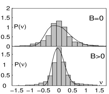
FIG. 1.: $\nu=(\Delta_{2}-<\Delta_{2}>)/\Delta$ - normalized peak spacings for $B=0$ and $B\neq 0$. Histograms are experimental data, solid lines - predictions of the interacting GSE (GUSE) for $B=0$ ($B\neq 0$)

We used RMT GUE distribution for $\epsilon_{N+1}-\epsilon_{N}$ and the Gaussian distribution for $u^{n}_{N+1,N+1}$, $u^{n}_{N,N}$ with the covariance $C_{nn}=0.069$. This value as well as $C_{np}$ and $C_{pp}$ below were obtained using a reasonable parametrization of the screened e-e interaction, [15].

For GSE the calculations required a proper treatment of the pairing $PT^{\dagger}T$ interaction appearing in the leading order in (15). This problem has an exact solution [16]. However we used a simple approximation which we felt was satisfactory. For even N we minimized this term in the subspace of two HF solutions with adjacent filled and empty Kramers pairs. We then formed an expectation of H with the resulting wave function. For the odd N the effect of the pairing is much simpler and the expectation with lowest energy HF wave function was sufficient. The resulting expressions are too cumbersome to record, cf., [15]. We used them with the RMT GSE statistics, $P=0.37\Delta$, the covariance $C_{nn}$ as in GUSE and $C_{pp}=0.023$, $C_{np}=0$.

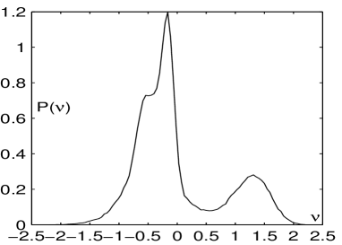
FIG. 2.: Normalized peak spacings for the interacting GUE

As one can see in Fig. 1 there no sign of the bimodal structure in the GSE and GUSE distributions. The reason for this in GUSE is perfectly obvious, cf., Eq. (31) - the spin degeneracy which is responsible for the bimodal structure in simple models of the CB is completely washed out by the combined effect of the SO interaction and the magnetic field. In the interacting GSE the non commutativity of the paring term $PT^{\dagger}T$ with the single particle part causes rather strong fluctuations relative to the RMT already in the lowest order. To appreciate this effect it is instructive to compare the leading GSE interaction terms, upper line in (15) with those of GUE, the upper line with $P=0$ in (11). The commuting spin interaction $J\hat{\bf S}^{2}$ does not change the basic RMT fluctuations but simply cuts and shifts different spin parts creating sharp structures. As seen in Fig. 2 these structures are washed out only partially by higher order terms. We conclude by observing that our results, Fig.1, fit quite poorly the tails of the spacing distributions. It is not clear to us if this is a consequence of our approximations in calculating $\Delta_{2}(N)$ or because of more fundamental reasons.

We wish to express our thanks to B.L. Altshuler, A. Finkelstein, K. Kikoin, Y.Oreg and J. da Providencia for useful discussions. V.B. and S.L. express their thanks for hospitality of University of Coimbra where part of this work was done. This work was supported in part by the DIP grant DIP-C 7.1. V.B. was supported in part by the NATO Science Fellowship Program CPRU18C00P0.

REFERENCES

[1] U. Sivan et al, Phys. Rev. Lett. 77, 1123 (1996); F.
Simmel at all, Europhys. Lett., 38, 123, (1997). S.M. Maurer et al,
Phys. Rev. Lett., 83, 1403, (1999), S.R. Patel et al., Phys. Rev. Lett.
80, 4522 (1998), F. Simmel, et al, Phys. Rev. B59, R10441 (1999).
[2] J. A. Folk et al, cond-mat/0010441, cf. also earlier worl on
spin effects in S. Tarucha et al., Phys. Rev. Lett. 77, 3613 (1996).
[3] I.L. Kurland, I.L. Aleiner, and B.L. Altshuler, Phys. Rev. B
62, 14886 (2000).
[4] P. W. Brouwer, Y. Oreg, and B. I. Halperin, Phys. Rev. B
60, R13977 (1999); B. I. Halperin et al, Phys. Rev. Lett., 86,
2106, (2001).
[5] D. Ullmo, and H. U. Baranger, cond-mat/0103098.
[6] Y.M. Blanter, A.D. Mirlin, and B.A. Muzykantskii, Phys. Rev.
Lett. 78, 2449 (1997).
[7] R. Berkovits, Phys. Rev. Lett. 81, 2128 (1998), A.
Cohen et al, Phys. Rev. B60, 2536 (1999), O. Prus, et al., B54,
R14281 (1996).
[8] S. Levit and D. Orgad, B60, 5549 (1999).
[9] P. Walker et al, Phys. Rev. Lett. 82, 5329 (1999), B60, 2541 (1999).
[10] M.L. Mehta, Random Matrices, (Academic Press, NY, 1991).
[11] C. Beenaker, Rev. Mod. Phys. 69, 731 (1997).
[12] Y. Alhassid, Rev. Mod. Phys. 72, 895 (2000).
[13] M.V. Berry, J. Phys. A 10, 2083 (1977).
[14] Ya.A Bychkov, and E.I. Rashba, JETP Lett. 39, 78,
(1984); L.I. Magarill, at al, JETP Lett. 72, 134, (2000).
[15] V.I. Belinicher, E. Ginossar, and S. Levit, to be published.
[16] R. W. Richardson, Phys. Lett. 159, 792 (1963).