Effective action approach and Carlson-Goldman mode in $d$-wave superconductors

Abstract

We theoretically investigate the Carlson-Goldman (CG) mode in two-dimensional clean $d$-wave superconductors using the effective “phase only” action formalism. In conventional $s$-wave superconductors, it is known that the CG mode is observed as a peak in the structure factor of the pair susceptibility $S(\Omega,\mathbf{K})$ only just below the transition temperature $T_{c}$ and only in dirty systems. On the other hand, our analytical results support the statement by Y. Ohashi and S. Takada, Phys. Rev. B 62, 5971 (2000) that in $d$-wave superconductors the CG mode can exist in clean systems down to the much lower temperatures, $T\approx 0.1T_{c}$. We also consider the manifestations of the CG mode in the density-density and current-current correlators and discuss the gauge independence of the obtained results.

I Introduction

More than 25 years ago, an unusual propagating sound-like ($\Omega/K=v_{\rm CG}$) Carlson-Goldman (CG) mode in charged superconducting systems with the velocity $v_{\rm CG}=10^{3}\,-\,10^{4}m/c$ was discovered Goldman.discovery (see also Goldman.1981 ). It was a widespread opinion before the CG mode discovery that since in the charged systems the sound-like Bogolyubov-Anderson (BA) Bogolyubov ; Anderson mode associated with neutral superconductors is converted to the plasma mode due to the Anderson-Higgs mechanism, there is no sound-like phase mode in charged systems.

A magnificent effort (see, for example, the reviews Artemenko ; book.1980 ; Galaiko ; book.1986 ) was made to understand the mechanism, responsible for the appearance of the CG mode and its relation to other phenomena of non-equilibrium superconductivity. While the majority theories of the CG mode Artemenko ; book.1980 ; Galaiko ; book.1986 ) were essentially based on the kinetic equations which are usually derived using the quasi-classical Green’s functions, the paper by Kulik, Entin-Wohlman, Orbach Kulik.1981 used a more conventional approach based on the Matsubara Green’s functions without kinetic equations. In the subsequent papers of Takada with coauthors (see Takada.1988 ; Takada.1997 and references therein) the approach of Kulik.1981 was further developed and very recently applied for the case of $d$-wave superconductivity Takada.2000 . The collective oscillations in $d$-wave superconductors were also studied using the kinetic equations for Green’s functions Artemenko.1997 (see also Artemenko.2001 ).

Since the discovery of high-$T_{c}$ compounds, the $d_{x^{2}-y^{2}}$ superconductivity has attracted much attention d-wave and the claim of Takada.2000 that the CG mode in clean $d$-wave superconductors may survive in a much wider region of temperatures down to $0.2T_{c}$ appears to be very different from the established properties of the CG mode in $s$-wave superconductors, so that it is important to check it by an independent calculation.

On the other hand, the importance of phase fluctuations in high-temperature superconductors (HTSC) (see, e.g. the review Loktev.review ), stimulated interest in the derivation of the “phase only” effective actions from the microscopic theory. It is important to emphasize that although there is no commonly accepted theory of HTSC, it seems reasonable that one can use a simple BCS-like approach to describe the properties of HTSC below the critical temperature, $T_{c}$ even though such an approach fails above $T_{c}$. Relying on this argument the “phase only” actions for $d$-wave superconductors were recently derived in Randeria.action ; we.LD ; Benfatto . However, the only phase excitations which are described by these actions are the BA mode in the neutral superconductor we.LD and the plasma mode Randeria.action ; Benfatto which appears when the Coulomb interaction is taken into account. This corresponds to the standard paradigm which does not yield the existence of the CG mode. Thus the purpose of the present paper is to investigate which ingredient is missing in the treatments of Randeria.action ; we.LD ; Benfatto , so that the CG mode does not appear in these approaches and to establish a link between the results of Takada.2000 and the “phase only” action formalism. This missing link is established here and the CG mode is obtained within the effective action formalism. Our main results can be summarized as follows.

1. We extend the “phase only” effective action formalism for charged systems to incorporate the density-current coupling which was so far considered only using other methods Kulik.1981 ; Takada.1988 ; Takada.1997 ; Takada.2000 (see also Varlamov.1986 ; Smith.1995 ; Smith.2000 , where the effect of this coupling appears to be important for the description of dirty superconductors). In neutral systems the density-current correlator does contribute in so called Landau terms of the effective action Aitchison.2000 ; we.LD , so that the correct expression for these terms can only be obtained when this correlator is taken into account.

2. We show that when the density-current coupling is included it becomes possible to obtain the CG mode using the “phase only” action. In particular, we derive an analytical expression for the pair susceptibility structure factor and solve numerically the equation for the CG mode velocity.

3. We show the gauge independent character of the equation for the collective phase excitations one of the solutions of which is the CG mode. Establishing a link between the pair susceptibility and this gauge independent equation for the phase excitations we argue that the peaks in the structure factor associated with the CG mode are independent of the choice of the gauge. The gauge independence of the equation for the CG mode used in the previous papers Takada.1988 ; Takada.1997 ; Takada.2000 is also shown applying the identity derived recently in Smith.2000 .

4. We consider possible manifestations of the CG mode in the gauge independent density-density and current-current response functions.

5. We derive analytical expressions for the density-density, current-current and density-current polarization functions for 2D clean $d$-wave superconductor at $T\ll T_{c}$.

The paper is organized as follows: In Sec. II we introduce our model. In Sec. III, we describe all details about the formalism used in the paper, necessary for further understanding. The various forms of the effective actions (for the phase and electric potential, “phase only” and “electric potential only”) are expressed in terms of density-density, current-current and density-current polarization functions in Sec. IV. The general expressions for these polarization functions are given in Appendix A, their derivation for $d$-wave superconductors is considered in Appendix C and the nodal approximation employed for this derivation is briefly discussed in Appendix B. In Sec. IV we also discuss in detail the difference between the present and other Kulik.1981 ; Takada.1988 ; Takada.1997 ; Takada.2000 ; Varlamov.1986 ; Smith.1995 ; Smith.2000 approaches. In Sec. V we briefly recall the properties of the phase excitations in the absence of the density-current coupling and stress some points like gauge independence of the equation for the collective phase excitations and the properties of the gauge independent density-density and current-current correlators which are particularly useful for better understanding of our main results which are presented in Sec. VI. In particular, in Sec. VI.1 we derive the equation for the CG mode, give its physical interpretation and discuss the gauge independence of the present and previous approaches. In Sec. VI.2 we present the results for the velocity of the CG mode and Sec. VI.3 is devoted to the structure factor (the calculational detail for these sections are given in Appendix D). We conclude in Sec. VII with a discussion and summary of our results.

II Model Hamiltonian

Let us consider the following action (in our notations the functional integral is expressed via $e^{S}$)

$$S=-\int_{0}^{\beta}d\tau\left[\sum_{\sigma}\int d^{2}r\psi_{\sigma}^{\dagger}(\tau,{\bf r})(\partial_{\tau}-ieA_{0}(\tau,{\bf r}))\psi_{\sigma}(\tau,{\bf r})+H(\tau)\right]\,,\qquad\mathbf{r}=(x,y)\,,\qquad\beta\equiv\frac{1}{T}\,,$$ (1)

where the Hamiltonian $H(\tau)$ is

$$\begin{split}H(\tau)&=\sum_{\sigma}\int d^{2}r\psi_{\sigma}^{\dagger}(\tau,{\bf r})[\varepsilon(-i\nabla-\frac{e}{c}{\bf A}(\tau,{\bf r}))-\mu]\psi_{\sigma}(\tau,{\bf r})\\ &-\frac{1}{2}\sum_{\sigma}\int d^{2}r_{1}\int d^{2}r_{2}\psi_{\sigma}^{\dagger}(\tau,{\bf r}_{2})\psi_{\bar{\sigma}}^{\dagger}(\tau,{\bf r}_{1})V({\bf r}_{1};{\bf r}_{2})\psi_{\bar{\sigma}}(\tau,{\bf r}_{1})\psi_{\sigma}(\tau,{\bf r}_{2})\\ &+\frac{1}{2}\int d^{2}r_{1}\int d^{2}r_{2}(\sum_{\sigma}\psi_{\sigma}^{\dagger}(\tau,{\bf r}_{1})\psi_{\sigma}(\tau,{\bf r}_{1})-n)V_{c}({\bf r}_{1}-{\bf r}_{2})(\sum_{\sigma^{\prime}}\psi_{\sigma^{\prime}}^{\dagger}(\tau,{\bf r}_{2})\psi_{\sigma^{\prime}}(\tau,{\bf r}_{2})-n)\,.\end{split}$$ (2)

Here $\psi_{\sigma}(\tau,{\bf r})$ is a fermion field with the spin $\sigma=\uparrow,\downarrow$, $\bar{\sigma}\equiv-\sigma$, $\tau$ is the imaginary time and $V({\bf r}_{1};{\bf r}_{2})$ is an attractive short-range potential, $V_{c}({\bf r}_{1}-{\bf r}_{2})$ is the long range Coulomb interaction, $n$ is the neutralizing background charge density. Throughout the paper we call the superconducting system neutral if the last term of Eq. (2) is omitted and charged if this term is taken into account. Even in the latter case the whole superconductor remains, of course, neutral due to the neutralizing ionic background.

We assume that the momentum representation of $V({\bf r}_{1};{\bf r}_{2})$ contains attraction only in the $d$-wave channel (see the discussion in Randeria.action ). The Fourier transform of the Coulomb interaction $V_{c}({\bf q})$ depends on the detail of the model. It can, for example, be taken $V_{c}({\bf q})=4\pi e^{2}/q^{2}$ in 3D, $V_{c}({\bf q})=2\pi e^{2}/q$ in 2D or more complicated expression (see e.g. Takada.2000 ; Randeria.action ) if the layered structure of HTSC is taken into account. However, the detailed expression is not crucial for the CG mode, because the mode appears when the Coulomb interaction is screened out by the quasiparticles. (The form of the expression would be, of course, essential for the analysis of the plasma mode Takada.1998 ; Randeria.action .) The form of dispersion law, $\varepsilon(\mathbf{k})$, is also not essential because the final results for the $d$-wave case will be formulated in terms of the non-interacting Fermi velocity $\mathbf{v}_{F}\equiv\partial\varepsilon(\mathbf{k})/\partial\mathbf{k}|_{\mathbf{k}=\mathbf{k}_{F}}$ and the gap velocity $\mathbf{v}_{\Delta}\equiv\partial\Delta(\mathbf{k})/\partial\mathbf{k}|_{\mathbf{k}=\mathbf{k}_{F}}$, where $\Delta(\mathbf{k})$ is the momentum dependent superconducting gap. We will also use the parameter $\alpha_{D}\equiv v_{F}/v_{\Delta}$ which is called the anisotropy of the Dirac cone. Throughout the paper $\hbar=k_{B}=1$ units are chosen. An external electromagnetic field $A=(A_{0},\mathbf{A})$ was introduced in the action Eq. (1) to calculate various correlation functions using the functional derivatives with respect to this external source field.

III Derivation of the effective action and the structure factor

The derivation of the effective “phase only” action for neutral (see e.g. Aitchison.2000 ; we.LD ; Loktev.review ) and charged Nagaosa.book ; Capezzali ; Randeria.action ; Benfatto $s$- and $d$-wave superconducting systems is widely discussed in the literature, so we briefly recap the main steps, including the functional integral representation for the structure factor, and making in Sec. IV a point on the appearance of the term which couples density and current.

The first step of the derivation is to use the appropriate Hubbard-Stratonovich transformations to decouple four-fermion interaction terms in the attractive and repulsive channels. The attractive part of the interaction was recently considered in detail in Sec. II of we.LD using the bilocal Hubbard-Stratonovich fields $\Phi(\tau,\mathbf{r}_{1};\mathbf{r}_{2})$ and $\Phi^{{\dagger}}(\tau,\mathbf{r}_{1};\mathbf{r}_{2})$ (see Kleinert for a review), so we show explicitly the corresponding transformation only for the Coulomb interaction:

$$\begin{split}&\exp\left[-\frac{1}{2}\int d\tau\int d^{2}r_{1}\int d^{2}r_{2}(\psi_{\sigma}^{\dagger}(\tau,\mathbf{r}_{1})\psi_{\sigma}(\tau,\mathbf{r}_{1})-n)V_{c}(\mathbf{r}_{1},\mathbf{r}_{2})(\psi_{\sigma^{\prime}}^{\dagger}(\tau,\mathbf{r}_{2})\psi_{\sigma^{\prime}}(\tau,\mathbf{r}_{2})-n)\right]=\\ &\int\mathcal{D}\varphi\exp\left\{-\int d\tau\int d^{2}r_{1}\int d^{2}r_{2}\left[\frac{1}{2}e\varphi(\tau,\mathbf{r}_{1})V_{c}^{-1}(\mathbf{r}_{1},\mathbf{r}_{2})e\varphi(\tau,\mathbf{r}_{2})-ie\varphi(\tau,\mathbf{r}_{1})(\psi_{\sigma}^{\dagger}(\tau,\mathbf{r}_{1})\psi_{\sigma}(\tau,\mathbf{r}_{1})-n)\delta(\mathbf{r}_{1}-\mathbf{r}_{2})\right]\right\}\,,\end{split}$$ (3)

where the Hubbard-Stratonovich field $\varphi$ has the meaning of the electric potential. Thus, the partition function is

$$\begin{split}Z=&\int\mathcal{D}\Psi^{\dagger}\mathcal{D}\Psi\mathcal{D}\Phi^{{\dagger}}\mathcal{D}\Phi\mathcal{D}\varphi\exp[S(\Psi^{\dagger},\Psi,\Phi^{\dagger},\Phi,\varphi,A)],\\ S&(\Psi^{\dagger},\Psi,\Phi^{\dagger},\Phi,\varphi,A)=\int_{0}^{\beta}d\tau\int d^{2}r_{1}\int d^{2}r_{2}\left\{-\frac{1}{V(\mathbf{r}_{1};\mathbf{r}_{2})}|\Phi(\tau,\mathbf{r}_{1};\mathbf{r}_{2})|^{2}-\frac{1}{2}e\varphi(\tau,\mathbf{r}_{1})V_{c}^{-1}(\mathbf{r}_{1},\mathbf{r}_{2})e\varphi(\tau,\mathbf{r}_{2})\right.\\ &+\Psi^{\dagger}(\tau,\mathbf{r}_{1})[-\partial_{\tau}+ie\tau_{3}A_{0}+ie\tau_{3}\varphi(\tau,\mathbf{r}_{1})-\tau_{3}\xi(-i\nabla-\tau_{3}\frac{e}{c}\mathbf{A})]\Psi(\tau,\mathbf{r}_{2})\delta(\mathbf{r}_{1}-\mathbf{r}_{2})\\ &\left.-ie\varphi(\tau,\mathbf{r}_{1})n\delta(\mathbf{r}_{1}-\mathbf{r}_{2})+\Phi^{{\dagger}}(\tau,\mathbf{r}_{1};\mathbf{r}_{2})\Psi^{\dagger}(\tau,\mathbf{r}_{1})\tau_{-}\Psi(\tau,\mathbf{r}_{2})+\Psi^{\dagger}(\tau,\mathbf{r}_{1})\tau_{+}\Psi(\tau,\mathbf{r}_{2})\Phi(\tau,\mathbf{r}_{1};\mathbf{r}_{2})\right\}\end{split}$$ (4)

where $\Psi$ and $\Psi^{\dagger}$ are the Nambu spinors, $\xi(-i\tau_{3}\nabla)\equiv\varepsilon(-i\tau_{3}\nabla)-\mu$ and $\tau_{3}$, $\tau_{\pm}=(\tau_{1}\pm i\tau_{2})/2$ are Pauli matrices.

To consider the Hubbard-Stratonovich field $\Phi$ it is convenient to use the relative $\mathbf{r}=\mathbf{r}_{1}-\mathbf{r}_{2}$ and center of mass coordinates $\mathbf{R}=(\mathbf{r}_{1}+\mathbf{r}_{2})/2$, so that $\Phi(\tau,\mathbf{r}_{1},\mathbf{r}_{2})\equiv\Phi(\tau,\mathbf{R},\mathbf{r})$. Now, using the functional integral representation, the imaginary time pair susceptibility is defined as

$$\eta(\tau,\mathbf{R}_{1}-\mathbf{R}_{2})=-\frac{1}{Z(A=0)}\int\mathcal{D}\Psi^{\dagger}\mathcal{D}\Psi\mathcal{D}\Phi^{{\dagger}}\mathcal{D}\Phi\mathcal{D}\varphi\Phi(\tau,\mathbf{R}_{1},\mathbf{0})\Phi^{\dagger}(0,\mathbf{R}_{2},\mathbf{0})\exp[S(\Psi^{\dagger},\Psi,\Phi^{\dagger},\Phi,\varphi)]\,.$$ (5)

Since the distance $|\mathbf{R}_{1}-\mathbf{R}_{2}|$ is expected to be larger than the internal Cooper pair scale, it is possible to put $\mathbf{r}=0$ in Eq. (5). The structure factor $S(\Omega,\mathbf{K})$ which used to present the experimental data Goldman.1981 ; book.1980 is related to the real frequency pair susceptibility $\eta(i\Omega_{n}\to\Omega+i0,\mathbf{K})$ by

$$S(\Omega,\mathbf{K})=-2[1-\exp(-\beta\Omega)]^{-1}\mbox{Im}\eta(\Omega+i0,\mathbf{K})\approx-\frac{2T}{\Omega}\mbox{Im}\eta(\Omega+i0,\mathbf{K})\,.$$ (6)

The definition of the pair susceptibility Eq. (5) is apparently gauge dependent, since the auxiliary Hubbard-Stratonovich field is gauge dependent. Nevertheless, as we discuss later the poles of $\eta(\Omega,\mathbf{K})$ are gauge independent and this justifies the use of Eqs. (5) and (6) to extract the observable values.

The simplest way to study the low energy phase dynamics foot1 is to employ the canonical gauge transformation foot2

$$\Psi(x)\to\begin{pmatrix}e^{i\theta(x)/2}&0\\ o&e^{-i\theta(x)/2}\end{pmatrix}\Upsilon(x),\qquad x\equiv(\tau,\mathbf{r})$$ (7)

separating the phase of the ordering field

$$\Phi(\tau,\mathbf{R},\mathbf{r})\approx\Delta(\tau,\mathbf{R},\mathbf{r})\exp[i\theta(\mathbf{\tau,R})]\,.$$ (8)

Then after the integration over the Fermi-fields the partition function becomes

$$Z=\int\Delta\mathcal{D}\Delta\mathcal{D}\theta\mathcal{D}\varphi\exp[-\beta\Omega\{\Delta,\partial\theta,\varphi,A\}]\,,$$ (9)

where the effective potential

$$\begin{split}\beta&\Omega\{\Delta,\partial\theta,\varphi,A\}=\\ &\int_{0}^{\beta}d\tau\int d^{2}r_{1}\int d^{2}r_{2}\left[\frac{\Delta^{2}(\tau,\mathbf{R},\mathbf{r})}{V(\mathbf{r}_{1}-\mathbf{r}_{2})}+\frac{1}{2}e\varphi(\tau,\mathbf{r}_{1})V_{c}^{-1}(\mathbf{r}_{1},\mathbf{r}_{2})e\varphi(\tau,\mathbf{r}_{2})+ie\varphi(\tau,\mathbf{r}_{1})n\delta(\mathbf{r}_{1}-\mathbf{r}_{2})\right]-\mbox{TrLn}G^{-1}\end{split}$$ (10)

with the inverse Green’s function

$$G^{-1}=\mathcal{G}^{-1}-\Sigma\,,$$ (11)

$$\begin{split}&\langle\tau_{1},\mathbf{r}_{1}|\Sigma(\partial\theta,\varphi,A)|\tau_{2},\mathbf{r}_{2}\rangle=\left[\tau_{3}\left(i\frac{\partial_{\tau_{1}}\theta}{2}-ie\varphi(\tau_{1},\mathbf{r}_{1})-ieA_{0}(\tau_{1},\mathbf{r}_{1})\right)+\tau_{3}O_{1}(\mathbf{r}_{1})+\hat{I}O_{2}(\mathbf{r}_{1})\right]\delta(\tau_{1}-\tau_{2})\delta(\mathbf{r}_{1}-\mathbf{r}_{2})\,.\end{split}$$ (12)

For $T\ll T_{c}$ it is reasonable to neglect the amplitude fluctuations and assume that the amplitude of the order parameter $\Delta(\tau,\mathbf{R},\mathbf{r})$ does not depend on $\mathbf{R}$. Then the frequency-momentum representation of $\mathcal{G}$ in Eq. (11) is the usual Nambu-Gor’kov Green’s function

$$\mathcal{G}(i\omega_{n},{\bf k})=-\frac{i\omega_{n}\hat{I}+\tau_{3}\xi({\bf k})-\tau_{1}\Delta(\mathbf{k})}{\omega_{n}^{2}+\xi^{2}({\bf k})+\Delta^{2}(\mathbf{k})}\,,$$ (13)

where, because $d$-wave pairing is considered $\Delta(\mathbf{k})=\Delta/2(\cos k_{x}a-\cos k_{y}a)$ ($a$ is the lattice constant) and $\omega_{n}=\pi(2n+1)T$ is fermionic (odd) Matsubara frequency. Since in what follows only the low temperatures, $T\ll\Delta(T)$ are considered, we can replace the temperature dependent amplitude $\Delta(T)$ by its zero temperature value, $\Delta_{0}\equiv\Delta(T=0)$. Thus all linear low temperature dependences of the polarization functions considered below are due to the nodes of $\Delta(\mathbf{k})$, but not to the temperature dependence of $\Delta(T)$ itself.

The precise form of the operators $O_{1}$ and $O_{2}$ in Eq. (12) which depends on the particular form of the tight-binding spectrum $\varepsilon(\mathbf{k})$ is given in we.LD (see also Benfatto for the formulation of the general rules for representation of $\Sigma$). It is essential, however, that the coordinate representation of $\Sigma$ does not depend on the phase $\theta$ itself and contains only its derivatives. Thus the coordinate representation of $\Omega_{kin}$ is also expressed via the derivatives of $\theta$. This property is particularly convenient for studying 2D models when a constant space independent phase is prohibited by the Coleman-Mermin-Wagner-Hohenberg (CMWH) theorem.

Since we are interested only in the phase dynamics in the presence of Coulomb interaction, in what follows we consider only the phase $\theta$ and the electric potential $\varphi$ dependent parts of the thermodynamical potential Eq. (10). This part of $\Omega$ which we denote as $\Omega_{kin}$ can be present as a series

$$\begin{split}\Omega_{kin}\{\partial\theta,\varphi\}=\int_{0}^{\beta}d\tau\int d^{2}r_{1}\int d^{2}r_{2}\left[\frac{1}{2}e\varphi(\tau,\mathbf{r}_{1})V_{c}^{-1}(\mathbf{r}_{1},\mathbf{r}_{2})e\varphi(\tau,\mathbf{r}_{2})+ie\varphi(\tau,\mathbf{r}_{1})n\delta(\mathbf{r}_{1}-\mathbf{r}_{2})\right]+T\mbox{Tr}\sum_{n=1}^{\infty}\frac{1}{n}({\cal G}\Sigma)^{n}\,.\end{split}$$ (14)

This way of deriving the effective action has many advantages. The main among them is that the gauge invariant combinations $\hbar\partial_{\tau}\theta/2-e\varphi-eA_{0}$ and $\hbar\nabla\theta/2-e/c\mathbf{A}$ are explicitly present during all stages of the derivation foot3 . This property is obviously related to the introduction of the phase via the gauge transformation Eq. (7). There is no need because of this to keep the external electromagnetic field $(A_{0},\mathbf{A})$ during the intermediate stages of the derivation since it can be easily restored following the above mentioned prescription which in the frequency-momentum space are

$$i\Omega_{n}\theta(K)\to i\Omega_{n}\theta(K)+2eA_{0}(K);\qquad iK_{\alpha}\theta(K)\to iK_{\alpha}\theta(K)-\frac{2e}{c}A_{\alpha}(K).$$ (15)

Differentiating with respect to this source field we will derive physical correlation functions (see the discussion in Randeria.action ) in what follows. It has to be stressed that the minimal coupling prescription (15) does not guaranty itself the gauge independence of the final result. The gauge independent treatment of the transformations (7) and (8) for $d$-wave pairing is, in particular, one of the complications foot2 .

In the previous studies of the CG mode Kulik.1981 ; Takada.1988 ; Takada.1997 ; Takada.2000 the phase field was introduced using the expansion of the ordering field $\Phi(x)$ around the equilibrium value $\Delta$ via $\Phi(x)=\Delta+\Phi_{1}(x)+i\Phi_{2}(x)$ and associating the fields $\Phi_{1}(x)$ with the amplitude and $\Phi_{2}(x)$ (or to be more precise $\Phi_{2}(x)/\Delta_{0}$) with the phase fluctuations. Although, as will be discussed below, the final result obtained in the both methods agrees, the present method of the investigation of the CG mode is more transparent because it explicitly uses the gauge independent combinations of the fields over the whole derivation. For example, one can easily recognize that $\Sigma$ contains a gauge independent Cooper pair chemical potential $\dot{\theta}/2-e\varphi$ book.1986 which in other approaches has to be collected from the different parts of the equations. Other advantages of the present approach will be discussed in the subsequent sections where the effective action is presented.

To consider the phase and charge fluctuations at the Gaussian level it is sufficient to include only the terms with $n=1,2$ in the infinite series in Eq. (14). Finally, we rewrite the pair susceptibility Eq. (5) in the new variables

$$\eta(\tau,\mathbf{R}_{1}-\mathbf{R}_{2})=-\int\Delta\mathcal{D}\Delta\mathcal{D}\theta\mathcal{D}\varphi\Delta(\tau,\mathbf{R}_{1},\mathbf{0})\exp[i\theta(\tau,\mathbf{R}_{1})]\Delta(0,\mathbf{R}_{2},\mathbf{0})\exp[-i\theta(\tau,\mathbf{R}_{2})]\exp[-\beta\Omega\{\Delta,\partial\theta,\varphi\}]\,.$$ (16)

As was mentioned above, we are interested only in the phase fluctuations structure factor neglecting the presence of the amplitude fluctuations. This implies that one can use a saddle point approximation for $\Delta$, so that omitting unimportant constant in the expansion of the exponent in Eq. (16) one arrives at

$$\eta(\tau,\mathbf{R}_{1}-\mathbf{R}_{2})=-\frac{\Delta_{0}^{2}}{4}\int\mathcal{D}\theta\mathcal{D}\varphi\theta(\tau,\mathbf{R}_{1})\theta(\tau,\mathbf{R}_{2})\exp[-\beta\Omega_{kin}\{\partial\theta,\varphi\}]\,.$$ (17)

Writing Eq. (17) we also expanded the exponents which were present in Eq. (16), because there are no free vortices in the system for $T<T_{c}$ and the multivalued character of the phase is irrelevant. This approximated form of the pair susceptibility is equivalent to the expressions for the susceptibility used in Refs. Kulik.1981 ; Takada.1988 ; Takada.1997 ; Takada.2000 . Expanding the exponents we neglect a widening of the structure factor peaks which is related to the absence of the long-range order in 2D (CMWH theorem). It is known, for example, from the analysis of the dynamic structure factor of lattices Mikeska ; Weling that $\delta$-function phonon resonance obtained in 3D harmonic crystals in 2D case is converted to the power law singularity

$$S(\omega,\mathbf{q})\sim\frac{f(\alpha)}{|\omega^{2}-v^{2}q^{2}|^{1-\alpha(T)}},$$ (18)

where $f(\alpha)$ is a function of $\alpha$ which goes to zero as $\alpha\to 0$, so that in this limit the structure factor transforms to $\delta$-function. Since for low temperatures $\alpha(T)\ll 1$ we may safely neglect this effect of widening because it does not move the position of the peak and we are primarily interested in the temperatures $T\ll T_{c}$.

IV General form of the effective action

In this section we present the effective potential $\Omega_{kin}\{\theta,\varphi\}$ and discuss the term which leads to the appearance of the CG mode. We also derive the effective “phase only” and “electric potential only” actions integrating out the electric potential $\varphi$ and the phase $\theta$, respectively.

IV.1 The effective action and polarization functions

Calculating the terms with $n=1,2$ in Eq. (14) (see e.g. Aitchison.2000 ; we.LD ) one arrives at

$$\begin{split}\beta\Omega_{kin}\{\theta,\varphi\}=\frac{T}{8}\sum_{n=-\infty}^{\infty}&\int\frac{d{\bf K}}{(2\pi)^{2}}\left[\varphi(-K)4e^{2}V_{c}^{-1}({\bf K})\varphi(K)+(i\Omega_{n}\theta(-K)-2e\varphi(-K))\Pi_{33}(K)(i\Omega_{n}\theta(K)+2e\varphi(K))\right.\\ &+\theta(-K)[\Lambda_{0}^{\alpha\beta}+\Pi_{00}^{\alpha\beta}(K)]K_{\alpha}K_{\beta}\theta(K)\\ &\left.+\theta(-K)(-K_{\alpha})\Pi_{30}^{\alpha}(K)(i\Omega_{n}\theta(K)+2e\varphi(K))+(i\Omega_{n}\theta(-K)-2e\varphi(-K))(-K_{\alpha})\Pi_{03}^{\alpha}(K)\theta(K)\right],\end{split}$$ (19)

where we introduced short-hand notations $K=(i\Omega_{n},{\bf K})$ with $\mathbf{K}$ being 2D vector (summation over dummy indices $\alpha,\beta=1,2$ is implied). In Eq. (19) the current-current polarization function, $\Pi_{00}$ is

$$\Pi_{00}^{\alpha\beta}(i\Omega_{n},{\bf K})\equiv T\sum_{l=-\infty}^{\infty}\int\frac{d^{2}k}{(2\pi)^{2}}\,\pi_{00}(i\Omega_{n},{\bf K};i\omega_{l},{\bf k})v_{F\alpha}({\bf k})v_{F\beta}({\bf k})\,$$ (20)

with the Fermi velocity $v_{F\alpha}(\mathbf{k})=\partial\xi(\mathbf{k})/\partial k_{\alpha}$; the density-density polarization function, $\Pi_{33}$ is

$$\Pi_{33}(i\Omega_{n},{\bf K})\equiv T\sum_{l=-\infty}^{\infty}\int\frac{d^{2}k}{(2\pi)^{2}}\,\pi_{33}(i\Omega_{n},{\bf K};i\omega_{l},{\bf k})\,$$ (21)

and the density-current polarization function, $\Pi_{03}^{\alpha}$ is

$$\Pi_{03}^{\alpha}(i\Omega_{n},{\bf K})\equiv T\sum_{l=-\infty}^{\infty}\int\frac{d^{2}k}{(2\pi)^{2}}\,\pi_{03}(i\Omega_{n},{\bf K};i\omega_{l},{\bf k})v_{F\alpha}({\bf k})\,.$$ (22)

$\pi_{ij}$ in Eqs. (20) - (22) is given by

$$\pi_{ij}(i\Omega_{n},{\bf K};i\omega_{l},{\bf k})\equiv\mbox{tr}[\mathcal{G}(i\omega_{l}+i\Omega_{n},{\bf k}+{\bf K}/2)\tau_{i}\mathcal{G}(i\omega_{l},{\bf k}-{\bf K}/2)\tau_{j}]\,,\qquad(\tau_{0}\equiv\hat{I})\,.$$ (23)

and $\Lambda_{0}^{\alpha\beta}$ in Eq. (19) is the first order contribution in the superfluid stiffness:

$$\Lambda_{0}^{\alpha\beta}=\int\frac{d^{2}k}{(2\pi)^{2}}n(\mathbf{k})m_{\alpha\beta}^{-1}(\mathbf{k}),\qquad m_{\alpha\beta}^{-1}(\mathbf{k})\equiv\partial^{2}\xi(\mathbf{k})/\partial k_{\alpha}\partial k_{\beta}$$ (24)

with

$$n(\mathbf{k})=1-\frac{\xi(\mathbf{k})}{E(\mathbf{k})}\tanh\frac{E(\mathbf{k})}{2T}\,,\qquad E(\mathbf{k})=\sqrt{\xi^{2}(\mathbf{k})+\Delta^{2}(\mathbf{k})}\,.$$ (25)

Writing Eq. (19) we omitted the linear time derivative term (see e.g. Randeria.action ; we.LD ) which is irrelevant for the present analysis.

The general expressions for the polarizations (20) - (22) are given in Appendix A (see also we.LD ) and calculated analytically for 2D clean $d$-wave superconductor in Appendix C (a brief discussion of the nodal approximation used to calculate these polarizations and the transformation to the global coordinate system are given in Appendices B and D, respectively).

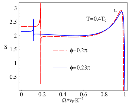
Figure 5: Structure factor $S(\Omega,\mathbf{K})$ in arbitrary units for $T=0.4T_{c}$. (a) $\Pi_{03}\neq 0$, (b) $\Pi_{03}=0$. The rest of the parameters is the same as in Fig. 3.

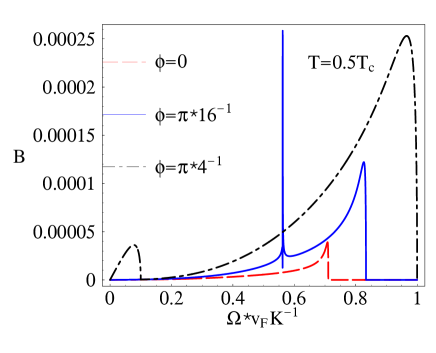
Figure 7: Spectral density $B(\Omega,\mathbf{K})$ in arbitrary but the same as in Fig. 6 units for $T=0.5T_{c}$. We put $\omega_{p}=0.5\epsilon_{F}$, $v_{F}K=0.001\epsilon_{F}$ (i.e. $\omega_{p}=500v_{F}K$) and $\alpha_{D}=10$.

As an example we show in Fig. 1 the real part of the density-density polarization function, $\Pi_{33}(\Omega,\mathbf{K})$ (this function is in fact just the Lindhard’s function for the superconducting state) which is given by Eq. (72) (and its dimensionless form by Eqs. (73) and (74)) as a function of $\Omega/v_{F}K$ for the different directions of $\mathbf{K}$. The angle $\phi$ determines the direction of $\mathbf{K}$ with respect to the $(10)$-direction in a such way that $\phi=\pi/4$ corresponds to the nodal direction (see also Eq. (85) and the explanation in Appendix D). Comparing this figure with Fig. 7 from Takada.2000 (our definition of $\phi$ is equivalent to the definition of the angle $\theta_{\mathbf{q}}$ used in Takada.2000 ), which was obtained by numerical integration of Eq. (60), one can see that our analytical expression (72) gives essentially the same result. In particular, Fig. 1 shows that $\Pi_{33}$ has a peak at $\Omega/v_{F}K=\cos(\phi-\pi/4)$. Furthermore, as shown, for instance, for $\phi=\pi/16$ there is a lower peak in $\mbox{Re}\Pi_{33}(\Omega,\mathbf{K})$ at $\Omega/v_{F}K=\cos(\phi-\pi/4+\pi/2)$. Note that the cases $\phi=0$ and $\phi=\pi/4$ are “degenerate” because for $\phi=0$ the lower peak coincides with the upper one and for $\phi=\pi/4$ the lower peak is at $\Omega/v_{F}K=0$ (see also Fig. 5, where the case $\phi=0.2,0.23\pi$ is shown).

In Takada.2000 the origin of these peaks was related to the gap nodes which can be regarded as two “one-dimensional normal state electronic bands” toward $\phi=\pm\pi/4$. These “normal bands” are able to screen out the Coulomb interaction in certain regions of the Fermi surface even for $T\ll T_{c}$ and this screening along with the presence of $\Pi_{03}^{\alpha}$ will make the appearance of the CG mode possible. Substituting Eq. (85) in the analytical expression (72) it is indeed easy to see that these peaks are due to the square root singularities of $\Pi_{33}$. These are the same singularities which are present in 2D normal state Lindhard’s function due to the lowered dimensionality of the momentum integration Tsvelik , but since $d$-wave superconducting state is considered the position of these singularities does depend on the direction of $\mathbf{K}$ with respect to the Fermi surface. Finally we note that these singularities in $\mbox{Re}\Pi_{33}$ at $\Omega=v_{F}K\cos(\phi-\pi/4)+0$ is accompanied by the singularity in $\mbox{Im}\Pi_{33}$ at $\Omega=v_{F}K\cos(\phi-\pi/4)-0$ which was considered in we.LD .

The effective potential Eq. (19) becomes more tractable in the matrix form

$$\beta\Omega_{kin}\{\theta,\varphi\}=\frac{T}{8}\sum_{n=-\infty}^{\infty}\int\frac{d{\bf K}}{(2\pi)^{2}}\begin{bmatrix}\theta(-K)\,\,&e\varphi(-K)\end{bmatrix}\mathcal{M}^{-1}\begin{bmatrix}\theta(K)\\ e\varphi(K)\end{bmatrix}\,,$$ (26)

where

$$\mathcal{M}^{-1}=\begin{bmatrix}-\Omega_{n}^{2}\Pi_{33}(K)+\Lambda^{\alpha\beta}(K)K_{\alpha}K_{\beta}-i\Omega_{n}K_{\alpha}\Pi_{03}^{\alpha}(K)-i\Omega_{n}K_{\alpha}\Pi_{30}^{\alpha}(K)&2i\Omega_{n}\Pi_{33}(K)-2K_{\alpha}\Pi_{30}^{\alpha}(K)\\ -2i\Omega_{n}\Pi_{33}(K)+2K_{\alpha}\Pi_{30}^{\alpha}(K)&4(-\Pi_{33}(K)+V_{c}^{-1}({\bf K}))\end{bmatrix}$$ (27)

with the bare (unrenormalized by the phase fluctuations) superfluid stiffness $\Lambda^{\alpha\beta}=\Lambda_{0}^{\alpha\beta}+\Pi_{00}^{\alpha\beta}(K)$.

IV.2 Comparison with other approaches

Let us compare our effective action Eqs. (26), (27) with the action obtained in Randeria.action and see the differences between the present and previous Kulik.1981 ; Takada.1988 ; Takada.1997 ; Takada.2000 approaches. As one can notice, the only difference between Eqs. (26), (27) and Eqs. (25), (26) in Randeria.action is due to the presence of the density-current polarization function, $\Pi_{03}^{\alpha}$. It is a general belief that this term has to be zero due to the “symmetry arguments” Nagaosa.book . However, as shown in Aitchison.2000 (see also we.LD , where the $d$-wave case is considered) this correlator has to be taken into account to obtain the correct expressions for the Landau terms of the effective action. This is the term which nontrivially couples phase and density fluctuations and makes the CG mode possible in the present approach.

From this point of view, the role of $\Pi_{03}^{\alpha}$ is the same as the role of the phase-charge coupling

$$\Pi_{23}(i\Omega_{n},{\bf K})\equiv T\sum_{l=-\infty}^{\infty}\int\frac{d^{2}k}{(2\pi)^{2}}\,\pi_{23}(i\Omega_{n},{\bf K};i\omega_{l},{\bf k})\gamma(\mathbf{k})\,,\qquad\gamma(\mathbf{k})\equiv\frac{2\Delta(\mathbf{k})}{\Delta_{0}},$$ (28)

with $\pi_{23}$ given by Eq. (23) in the approach of Kulik et al. Kulik.1981 and Takada with coauthors Takada.1988 ; Takada.1997 ; Takada.2000 . Note that $\Pi_{23}=-\Pi_{32}$, while $\Pi_{03}^{\alpha}=\Pi_{30}^{\alpha}$.

It is interesting that techniques essentially similar with Kulik.1981 ; Takada.1988 ; Takada.1997 ; Takada.2000 have been used in Varlamov.1986 and Smith.1995 ; Smith.2000 to consider suppression of the critical temperature in disordered superconductors. In Smith.1995 ; Smith.2000 both amplitude and phase fluctuations were taken into account and to consider the influence of nonmagnetic impurities the electronic Green’s functions had $4\times 4$ matrix structure. The main difference between Kulik.1981 ; Takada.1988 ; Takada.1997 ; Takada.2000 ; Varlamov.1986 ; Smith.1995 ; Smith.2000 , nevertheless, remained the same, viz. the order parameter phase was expressed via the operator $O_{2}=\Psi^{\dagger}\tau_{2}\Psi$, as summarized in Table II of Smith.1995 . Thus $\tau_{2}$ also enters the phase-density correlator, $\Pi_{23}$ in the notations of Kulik.1981 ; Takada.1988 ; Takada.1997 ; Takada.2000 (or $\Pi_{\phi\rho}$ in the notations of Smith.1995 ; Smith.2000 ).

In our opinion, the physical meaning of $\Pi_{23}$ is, however, more obscure than that of $\Pi_{03}^{\alpha}$. Indeed, since $\Pi_{23}$ is expressed via the Pauli matrix $\tau_{2}$, so that it seems like the phase itself is a dynamical variable on its own, while physically meaningful are only the space and time derivatives of the phase.

These derivatives can only enter into the formal expressions as a current via $\hat{I}$ and as a density via $\tau_{3}$ matrices, respectively. This property is obviously present in the definition Eq. (22) of $\Pi_{03}^{\alpha}$ which thus has the more clear meaning of a density-current polarization function.

Another important difference between the present and previous Kulik.1981 ; Takada.1988 ; Takada.1997 ; Takada.2000 ; Varlamov.1986 ; Smith.1995 ; Smith.2000 approaches is that the present derivation does not need an explicit use of the gap equation for $\Delta$. For example, in Kulik.1981 the charge conservation follows from the explicit use of the gap equation, while in the present approach as we will discuss later, the charge conservation is already built in the phase dynamics itself.

The fact that the present approach does not rely on the particular form of the gap equation is more convenient for modeling HTSC, where the gap does not close at the critical temperature $T_{c}$, so that the equation $\Delta(T_{c}^{0})=0$ gives only the mean-field transition temperature, $T_{c}^{0}$. Thus another definition of the true critical temperature, $T_{c}$ is necessary. As recently discussed in Benfatto.dissipation (see also Loktev.review ), it is reasonable for HTSC to estimate $T_{c}$ as the temperature of the Berezinskii-Kosterlitz-Thouless transition (see Eq. (79) in Appendix C).

Finally, it is worth to mention here the recent papers Gusynin , where the approach very similar to that of the present paper was employed to study the CG mode in the model of color superconducting quark matter. One of the advantages of Gusynin is that it treats the problem in an explicitly gauge invariant way, while here, the Coulomb gauge is already imposed in writing the Hamiltonian Eq. (2) and then, when necessary, the gauge independence of the results obtained is discussed in a more intuitive way. In general, however, to prove the gauge independence of the results an arbitrary gauge has to be considered, to show that the physical observables do not depend on the gauge fixing parameter as done in Gusynin (see also Aitchison.1984 , where the gauge invariance of the physical quantities calculated using the $T=0$ effective potential is discussed). Following this route one can obtain the “relativistic” (see the second paper in Gusynin for the details of the proof) generalization of Eq. (19) which contains a gauge fixing parameter $\lambda$

$$\begin{split}\beta\Omega_{kin}\{\theta,A_{\mu}\}=&T\sum_{K}\frac{1}{8}\left\{\frac{1}{\pi}\left[A_{\mu}(-K)(K^{2}\delta_{\mu\nu}-K_{\mu}K_{\nu})A_{\nu}(K)+\frac{1}{\lambda}A_{\mu}(-K)K_{\mu}K_{\nu}A_{\nu}(K)\right]\right.\\ &\left.+(-iK_{\mu}\theta(-K)-2eA_{\mu}(-K))\Pi_{\mu\nu}(K)(iK_{\nu}\theta(K)-2eA_{\nu}(K))\right\},\end{split}$$ (29)

with $K_{\mu}\equiv(\Omega_{n},\mathbf{K})$, $K^{2}=K_{\mu}K_{\mu}=\Omega_{n}^{2}+\mathbf{K}^{2}$, $\mu,\nu=0,1,2$ and $A_{0}(K)=-\varphi(K)$ and $c=1$. Note that in Eq. (29) we have the whole electromagnetic potential $A_{\mu}$ instead of the Coulomb component present in Eq. (19). The polarization tensor $\Pi_{\mu\nu}(K)$ is obviously related to the polarizations used in Eq. (19). The question of gauge independence (or dependence) can be addressed considering how the calculated quantities depend on $\lambda$.

IV.3 Effective actions for the phase and electric potential

Integrating out $\varphi$ and $\theta$ from Eq. (26) one can obtain, respectively

$$\beta\Omega_{kin}\{\theta\}=\frac{T}{8}\sum_{n=-\infty}^{\infty}\int\frac{d{\bf K}}{(2\pi)^{2}}\theta(-K)\mathcal{M}_{\theta}^{-1}(i\Omega_{n},\mathbf{K})\theta(K),\qquad\mathcal{M}_{\theta}^{-1}=M_{11}^{-1}-M_{22}M_{12}^{-1}M_{21}^{-1}$$ (30)

and

$$\beta\Omega_{kin}\{\varphi\}=\frac{T}{8}\sum_{n=-\infty}^{\infty}\int\frac{d{\bf K}}{(2\pi)^{2}}\varphi(-K)\mathcal{M}_{\varphi}^{-1}(i\Omega_{n},\mathbf{K})\varphi(K),\qquad\mathcal{M}_{\varphi}^{-1}=e^{2}(M_{22}^{-1}-M_{11}M_{12}^{-1}M_{21}^{-1})\,.$$ (31)

It is evident that $\mathcal{M}_{\varphi}^{-1}=e^{2}M_{22}^{-1}M_{11}\mathcal{M}_{\theta}^{-1}=e^{2}M_{22}^{-1}\mbox{det}\mathcal{M}^{-1}$, so that if $M_{11}^{-1},M_{22}^{-1}\neq 0$ the equations $\mathcal{M}_{\theta}^{-1}=\mathcal{M}_{\varphi}^{-1}=\mbox{det}\mathcal{M}^{-1}=0$ are equivalent.

Using Eqs. (17) and (31) it is straightforward to obtain that the structure factor Eq. (6) is given by

$$S(\Omega,\mathbf{K})=\frac{T}{\Omega}\frac{\Delta_{0}^{2}}{8}\mbox{Im}\mathcal{M}_{\theta}(\Omega+i0,\mathbf{K})\,.$$ (32)

V Phase excitations in the charged system in the absence of the density-current coupling

V.1 Equation for the collective phase excitations

Let us assume for a moment that there is no density-current coupling ($\Pi_{03}^{\alpha}=\Pi_{30}^{\alpha}=0$) and discuss briefly the collective excitations which follow from Eqs. (27), (30) and (31). As mentioned above the matrix $\mathcal{M}^{-1}$ reduces in this case to the known expression Randeria.action . Therefore, it is not surprising that the “phase only” action Eq. (30) takes the form

$$\mathcal{M}_{\theta}^{-1}(i\Omega_{n},{\bf K})=-\Omega_{n}^{2}\mathbf{\bar{\Pi}}_{33}+\Lambda^{\alpha\beta}K_{\alpha}K_{\beta},\qquad\mathbf{\bar{\Pi}}_{33}=\frac{\Pi_{33}(K)}{1-\Pi_{33}(K)V_{c}({\bf K})}\,,$$ (33)

which coincides with the corresponding expression in Randeria.action (see also Nagaosa.book ). The dispersion law of the collective phase modes is defined by the equation

$$\mathcal{M}_{\theta}^{-1}(i\Omega_{n}\to\Omega+i0,{\bf K})=0.$$ (34)

This equation can also be regarded as a direct consequence of the charge conservation

$$\frac{\partial\rho(t,\mathbf{r})}{\partial t}+\nabla\cdot\mathbf{j}(t,\mathbf{r})=0\,,$$ (35)

where the current and charge density are defined via

$$\mathbf{j}=-c\frac{\delta\Omega_{kin}\{\theta,A\}}{\delta\mathbf{A}},\qquad\rho=\frac{\delta\Omega_{kin}\{\theta,A\}}{\delta A_{0}}\,,$$ (36)

where the electromagnetic field $A$ in $\Omega_{kin}$ was restored using the rule Eq. (15). Evaluating Eq. (36) one arrives at Eq. (45) with $\Pi_{03}^{\alpha}=0$, so that Eq. (34) is indeed recovered. There is, in fact, no surprise in the link between Eqs. (35) and (34) which is just the consequence of the way how we introduced the phase $\theta$ in Eq. (7).

As discussed in Randeria.action ; Nagaosa.book the only solution of this equation for $\mathbf{K}\to 0$ is the plasma mode. Using as an example the 3D form of the Coulomb potential and assuming that $\Lambda^{\alpha\beta}=\Lambda\delta_{\alpha\beta}$ which is valid for isotropic system with $m_{\alpha\beta}=m\delta_{\alpha\beta}$, one obtains from this equation that the plasma frequency, $\omega_{p}=\sqrt{4\pi\Lambda e^{2}}$ for the limit $\mathbf{K}\to 0$. The expression for $\omega_{p}$ can be reduced to the standard $\sqrt{4\pi ne^{2}/m}$ if one uses the superfluid stiffness $\Lambda=n/m$ obtained for the continuum model with $s$-wave pairing.

It is clear that for the plasma mode $\Omega_{p}(\mathbf{K})/K\to\infty$ as $\mathbf{K}\to 0$. This property remains valid even if 2D Coulomb potential is used and it makes plasmons different from any sound mode with $\Omega/K\to\mbox{const}$ as $\mathbf{K}\to 0$. For example, if a neutral superconductor were considered the polarization $\mathbf{\bar{\Pi}}_{33}$ in Eq. (33) would be replaced by $\Pi_{33}$ and the solution of Eq. (34) for $\mathbf{K}\to 0$ is the sound-like BA mode and its velocity is given by Eq. (78).

V.2 Phase excitations via electric potential propagator and gauge independent density-density and current-current correlators

It is instructive also to look at the form $\mathcal{M}_{\varphi}$ for the electric potential $\varphi$ which is

$$\begin{split}\mathcal{M}_{\varphi}^{-1}(i\Omega_{n},{\bf K})=4e^{2}\left(\frac{-\Pi_{33}\Lambda^{\alpha\beta}K_{\alpha}K_{\beta}}{-\Omega_{n}^{2}\Pi_{33}+\Lambda^{\alpha\beta}K_{\alpha}K_{\beta}}+V_{c}^{-1}(\mathbf{K})\right)\,.\end{split}$$ (37)

Considering the same example of isotropic system with 3D Coulomb potential Eq. (37) in the limit $\mathbf{K}\to 0$ and $\Omega/K\to\infty$ can be reduced to the known expression (see e.g. Nagaosa.book )

$$\mathcal{M}_{\varphi}^{-1}(i\Omega_{n},{\bf K})=\frac{\mathbf{K}^{2}}{\pi}\left(1+\frac{\omega_{p}^{2}}{\Omega_{n}^{2}}\right)\,.$$ (38)

It is obvious that the discussed above plasma mode can be also seen in $\mathcal{M}_{\varphi}$. Indeed after the analytical continuation $i\Omega_{n}\to\Omega+i0$, $\mathcal{M}_{\varphi}(\Omega,\mathbf{K})$ acquires a pole at $\Omega=\omega_{p}$.

It is also useful to evaluate gauge independent density-density and current-current correlators which are defined as

$$\chi(i\Omega_{n},{\bf K})=-\frac{\delta^{2}T\ln Z\{A\}}{\delta A_{0}(-K)\delta A_{0}(K)},\qquad\chi^{\alpha\beta}(i\Omega_{n},{\bf K})=-\frac{\delta^{2}T\ln Z\{A\}}{\delta A_{\alpha}(-K)\delta A_{\beta}(K)},$$ (39)

where

$$Z\{A\}=\int\mathcal{D}\theta\mathcal{D}\varphi\exp[-\beta\Omega_{kin}\{\theta,\varphi,A\}]$$ (40)

with the external field $(A_{0},\mathbf{A})$ restored using the rule Eq. (15). Then we arrive at the standard expressions Randeria.action

$$\chi(i\Omega_{n},{\bf K})=-\frac{e^{2}\mathbf{\bar{\Pi}}_{33}\Lambda^{\alpha\beta}K_{\alpha}K_{\beta}}{\Lambda^{\alpha\beta}K_{\alpha}K_{\beta}-\mathbf{\bar{\Pi}}_{33}\Omega_{n}^{2}}$$ (41)

and

$$\chi^{\alpha\beta}(i\Omega_{n},{\bf K})=e^{2}\left(\Lambda^{\alpha\beta}-\frac{\Lambda^{\alpha\mu}\Lambda^{\nu\beta}K_{\mu}K_{\nu}}{-\Omega_{n}^{2}\mathbf{\bar{\Pi}}_{33}+\Lambda^{\alpha\beta}K_{\alpha}K_{\beta}}\right)\,.$$ (42)

Again assuming that $\Lambda^{\alpha\beta}=\Lambda\delta_{\alpha\beta}$ one can reduce Eq. (42) to the known form of the current-current correlator

$$\chi^{\alpha\beta}(i\Omega_{n},{\bf K})=e^{2}\Lambda\frac{-\Omega_{n}^{2}\mathbf{\bar{\Pi}}_{33}\delta_{\alpha\beta}+\Lambda K^{2}\left(\delta_{\alpha\beta}-\frac{K_{\alpha}K_{\beta}}{K^{2}}\right)}{-\Omega_{n}^{2}\mathbf{\bar{\Pi}}_{33}+\Lambda K^{2}}.$$ (43)

The difference between gauge independent Eq. (41) and Eq. (42) and gauge dependent $\mathbf{\bar{\Pi}}_{33}$, $\Lambda^{\alpha\beta}$ in Eq. (33) was recently discussed in Randeria.action . The link considered above between charge conservation Eq. (35) and Eq. (34) shows that the solutions of Eq. (34) are gauge independent, even though $\mathbf{\bar{\Pi}}_{33}$, $\Lambda^{\alpha\beta}$ are gauge dependent. At the more formal level it can be argued that Eqs. (41) and (42) are gauge independent because even if one derives them starting from Eq. (29) the gauge fixing parameter $\lambda$ does not enter the final result and one obtains the same expressions.

The putting this in another way, one can say that the position of zeros of $\mathcal{M}_{\theta}^{-1}(\Omega,\mathbf{K})$ is gauge independent, because these zeros coincide with the poles of the gauge independent $\chi(\Omega,\mathbf{K})$. As we will see in Sec. VI.4, density-current coupling modifies both Eqs. (41) and (42), nevertheless the general argument about zeros of $\mathcal{M}_{\theta}^{-1}(\Omega,\mathbf{K})$ (poles of $\mathcal{M}_{\theta}(\Omega,\mathbf{K})$) remains valid.

VI Phase excitations in the presence of the density-current coupling

Here we generalize all expressions from the previous section for nonzero $\Pi_{30}^{\alpha}$. In particular, Eq. (33) becomes

$$\begin{split}&\mathcal{M}_{\theta}^{-1}(i\Omega_{n},{\bf K})=-\Omega_{n}^{2}\mathbf{\bar{\Pi}}_{33}-i\Omega_{n}K_{\alpha}(\mathbf{\bar{\Pi}}_{03}^{\alpha}(K)+\mathbf{\bar{\Pi}}_{30}^{\alpha}(K))+\mathbf{\bar{\Lambda}}^{\alpha\beta}K_{\alpha}K_{\beta},\\ &\mathbf{\bar{\Pi}}_{03}^{\alpha}(K)\equiv\frac{\Pi_{03}^{\alpha}(K)}{1-\Pi_{33}(K)V_{c}({\bf K})},\qquad\mathbf{\bar{\Lambda}}^{\alpha\beta}\equiv\Lambda^{\alpha\beta}+\frac{\Pi_{03}^{\alpha}(K)\Pi_{30}^{\beta}(K)}{-\Pi_{33}(K)+V_{c}^{-1}({\bf K})}.\end{split}$$ (44)

The dispersion law for all collective phase excitations is still defined by Eq. (34), but with $\mathcal{M}_{\theta}$ given by Eq. (44). It has to be pointed out that the interpretation of Eqs. (34) and (44) as the charge conservation law Eq. (35) remains valid even for $\Pi_{30}^{\alpha}\neq 0$. The only difference is that the expressions (36) for current and density

$$j_{\alpha}(i\Omega_{n},\mathbf{K})=\frac{e}{2}(\mathbf{\bar{\Lambda}}^{\alpha\beta}(K)iK_{\beta}-i\mathbf{\bar{\Pi}}_{03}^{\alpha}(K)i\Omega_{n})\theta(K),\qquad\rho(i\Omega_{n},\mathbf{K})=-\frac{e}{2}(\mathbf{\bar{\Pi}}_{33}(K)i\Omega_{n}+i\mathbf{\bar{\Pi}}_{03}^{\alpha}(K)iK_{\alpha})\theta(K)$$ (45)

are now more complicated and contain $\mathbf{\bar{\Pi}}_{03}^{\alpha}$. Nevertheless substitution of Eq. (45) in Eq. (35) indeed results in Eq. (34) with $\mathcal{M}_{\theta}$ given by Eq. (44). Hence, even in the most general case $\Pi_{03}^{\alpha}\neq 0$ the position of zeros of $M_{\theta}^{-1}$ (poles of $M_{\theta}$) is gauge independent.

VI.1 Equation for the CG mode, its physical interpretation and gauge independence

It can be checked that in the limit $\mathbf{K}\to 0$ and $\Omega/K\to\infty$ one of the collective modes is the plasma mode considered above. We are, however, more interested whether a sound-like mode ($\Omega/K=\mbox{const}$ for $\mbox{K}\to 0$) which would be similar to the BA mode in neutral superconductors can exist in the charged system. It is seen from Eq. (44) that if the ratio $\Omega/K$ is fixed and one is interested in the low energy excitations with $\Omega\to 0$, only the last term of Eq. (44) is relevant because $\mathbf{{\bar{\Pi}}}_{33}(K)$ and $\mathbf{{\bar{\Pi}}}_{03}^{\alpha}(K)$ are $\sim V_{c}^{-1}(\mathbf{K})$ in this limit. In this case the equation $\mathcal{M}_{\theta}^{-1}(\Omega,{\bf K})=0$ after the analytical continuation $i\Omega_{n}\to\Omega+i0$ reduces to

$$\mathbf{\bar{\Lambda}}^{\alpha\beta}(\Omega,\mathbf{K})K_{\alpha}K_{\beta}=\left(\Lambda^{\alpha\beta}(\Omega,\mathbf{K})-\frac{\Pi_{03}^{\alpha}(\Omega,\mathbf{K})\Pi_{30}^{\beta}(\Omega,\mathbf{K})}{\Pi_{33}(\Omega,\mathbf{K})}\right)K_{\alpha}K_{\beta}=0,$$ (46)

so that the detailed form of the Coulomb interaction becomes irrelevant, as was mentioned above. The solutions of Eq. (46) are gauge independent because for $\mathbf{K\to 0}$ this equation is equivalent to the gauge independent equation $\mathcal{M}_{\theta}^{-1}(\Omega,{\bf K})=0$.

It is interesting that practically the same arguments about the gauge independence of the CG mode studied using the formalism of Refs. Kulik.1981 ; Takada.1988 ; Takada.1997 ; Takada.2000 can be made. The corresponding equation for the CG mode is

$$\mathbf{\bar{\Pi}}_{22}(\Omega,\mathbf{K})-\Pi_{22}(0,\mathbf{0})=0,$$ (47)

where

$$\mathbf{\bar{\Pi}}_{22}(\Omega,\mathbf{K})=\Pi_{22}(\Omega,\mathbf{K})+\Pi_{23}(\Omega,\mathbf{K})\frac{V_{c}(\mathbf{K})}{1-V_{c}(\mathbf{K})\Pi_{33}(\Omega,\mathbf{K})}\Pi_{32}(\Omega,\mathbf{K})$$ (48)

$\Pi_{23}$ is given by Eq. (28) and the definition of $\Pi_{22}$ is given in Takada.2000 (in addition to two obvious $\tau_{2}$ matrices it also contains the factor $\gamma^{2}(\mathbf{k})$ because $d$-wave pairing is considered). One can show that in the limit $\mathbf{K}\to 0$ equation (47) reduces to the Ward identity

$$[-2/V+\Pi_{22}(\Omega,\mathbf{K}\to 0)]\Pi_{33}(\Omega,\mathbf{K}\to 0)+\Pi_{23}^{2}(\Omega,\mathbf{K}\to 0)=0\,.$$ (49)

Exactly this identity was recently proven in Smith.2000 (to be precise, $s$-wave pairing was considered in Smith.2000 ) using the gauge independence (charge conservation) arguments (see e.g. Schrieffer ) and the mean field gap equation

$$\frac{2}{V}+\Pi_{22}(0,\mathbf{0})=0.$$ (50)

As was already mentioned the last equation has to be explicitly used in the formalism of Kulik.1981 ; Takada.1988 ; Takada.1997 ; Takada.2000 .

It is possible to establish a link between Eq. (46) and a simple and transparent interpretation of the CG mode suggested by Schmid and Schön Schmid.1975 (see also Chap. 13 in book.1986 ). Comparing the expression for current in Eq. (45) and Eq. (46) one can notice that since $\mathbf{{\bar{\Pi}}}_{03}^{\alpha}(K)$ disappears in the limit $\mathbf{K}\to 0$, Eq. (46) is just a condition

$$\nabla\cdot\mathbf{j}=0,\qquad j_{\alpha}(i\Omega_{n},\mathbf{K})=\frac{e}{2}\mathbf{\bar{\Lambda}}^{\alpha\beta}(K)iK_{\beta}\theta(K)$$ (51)

which implies that if there is a supercurrent in the system, it should be compensated by some normal current minimizing the total current. Exactly the same condition which relates the CG mode to a counterflow of supercurrent and normal current is discussed in book.1986 . Thus using the two fluid picture one may say that $\mathbf{\bar{\Lambda}}^{\alpha\beta}(K)$ in Eq. (46) consists of the supercurrent $\Lambda^{\alpha\beta}$ and normal $\mathbf{\bar{\Lambda}}^{\alpha\beta}(K)-\Lambda^{\alpha\beta}(K)$ parts, respectively.

Although this counterflow resembles second sound in He⁴, it was pointed out in the earliest studies Schmid.1975 (see also book.1980 ; book.1986 ) that the CG mode is not the second sound which is a hydrodynamic mode since in the CG mode the normal fluid and superfluid are not in the local thermodynamic equilibrium and this mode is not a hydrodynamic mode.

It has to be stressed that even though the solutions of Eqs. (46) and (47) are gauge independent for $\mathbf{K}\to 0$, the existence of such solutions is not required by the gauge invariance because no general statement can be made about the polarizations $\Pi_{33}$, $\Lambda^{\alpha\beta}$ and $\Pi_{03}^{\alpha}$ for arbitrary values of $\Omega$ and $\mathbf{K}$. Thus, in contrast to the BA and plasma modes the existence of which is guaranteed by the Goldstone theorem foot4 and Anderson-Higgs mechanism, the CG mode does not obey any theorem and its existence is a fortunate result of many subtle features of the system dynamics.

VI.2 Velocity of the CG mode

It is difficult to solve Eq. (46) analytically for $d$-wave pairing and even numerically a more simple equation for real part, $\mbox{Re}\mathbf{\bar{\Lambda}}^{\alpha\beta}(\Omega,\mathbf{K})=0$ is usually considered Takada.1997 ; Takada.2000 . This significantly simplifies its solution, but in general this approximation can be justified only a posteriory, when the imaginary part is estimated. It is possible to study this equation in two ways. The first way is to extract the dispersion law $\Omega(\mathbf{K})$ for, in general, arbitrary $\mathbf{K}$. The second way is to find the velocity of the CG mode, $v_{CG}(\phi)\equiv\Omega/|\mathbf{K}|$ in the limit $\mathbf{K}\to 0$. The extraction of the dispersion law is more sensitive to the approximations which were made in the calculation of the polarization operators. In particular, usage of the approximated expressions (62), (63) and (64), which neglect the pair breaking for $\Omega\geq 2\Delta_{0}$, introduces the restriction $v_{F}K<\Delta_{0}$. Moreover, for the polarizations Eqs. (73), (76) and (80) calculated using the nodal approximation (see Appendix B) the condition of smallness of $\mathbf{K}$ becomes even more strict, so that here we study only the equation for $v_{CG}$. As also discussed in Appendix B the nodal approximation is valid for $T\ll\Delta_{0}$. This is the reason why in the present paper only the temperatures $T<0.6T_{c}$ are considered, where $T_{c}$ is defined by Eq. (79). Nevertheless, the presented formalism allows in principle to study the phase fluctuation structure factor up to $T_{c}$ if no additional approximations are made in calculation of the polarizations.

Thus for the illustrative purpose and comparison with Takada.2000 we also solve numerically the equation

$$\mbox{Re}\mathbf{\bar{\Lambda}}^{\alpha\beta}\left(\frac{\Omega}{K}=v_{CG}(\phi),K\to 0\right)\frac{K_{\alpha}K_{\beta}}{K^{2}}=0$$ (52)

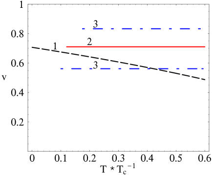
Figure 2: Temperature dependence of the velocities of the BA mode (dashed line – $1$), the CG mode for $\phi=0$ (full line – $2$) and $\phi=\pi/16$ (dot-dashed lines – $3$). We put $\alpha_{D}=10$ and the velocities are expressed in units of $v_{F}$.

(it is rewritten in dimensionless form (81) for the numerical work) instead of Eq. (46) and the results are presented in Fig. 2. We stress that for $\phi=\pi/16$ we obtain two solutions: $v_{CG}\approx 0.83v_{F}$ and $v_{CG}\approx 0.56v_{F}$. These results are in fact in a very good agreement with the results shown in Figs. 2 (a) and (b) of Takada.2000 . In particular, we also obtain that the velocity of the CG mode is practically temperature independent and its value is well described by $v_{CG}=v_{F}\cos(\phi-\pi/4)$ (or $v_{CG}^{\prime}=v_{F}\cos(\phi-\pi/4+\pi/2)$ for the other pair of nodes which is rotated with respect to the first pair by $\pi/2$). Indeed, this equation gives

$$v_{CG}=v_{F}\times\left\{\begin{array}[]{cccclc}0.707&(0.711&\mbox{at}&T=0.5T_{c})&:\phi=0&(\mbox{antinodal direction})\\ 0.831&(0.833&\mbox{at}&T=0.5T_{c})&:\phi=\pi/16&\\ 0.555&(0.562&\mbox{at}&T=0.5T_{c})&:\phi=\pi/16&(\mbox{other pair of nodes})\\ 1&(1.00&\mbox{at}&T=0.5T_{c})&:\phi=\pi/4&(\mbox{nodal direction})\end{array}\right.$$ (53)

Interestingly we obtain that the CG mode disappears even at somewhat lower temperature than in Takada.2000 , $T=0.1T_{c}$. This lowest value of $T$ when the CG mode still exists is, however, more the result of numerical solution of Eq. (52) than a real threshold temperature, because the peaks of the structure factor considered below disappear rather gradually.

VI.3 Structure factor

The knowledge of the structure factor $S(\Omega,\mathbf{K})$ is even more important than the value of the velocity, $v_{CG}$, because this factor contains the information about the damping of the CG mode foot5 . Furthermore, as we already mentioned, this is the quantity which is measured in the Carlson-Goldman experiment Goldman.discovery ; Goldman.1981 .

One of the main results of the present paper is that we obtain a closed analytical expression for the structure factor (32) for the clean $d$-wave superconductor which is just a substitution of $\Pi_{33}$, $\Pi_{03}^{\alpha}$ and $\Lambda$ given by Eqs. (73), (80), (76) in Eqs. (44) and (44) (its inverse imaginary part) in Eq. (32), respectively. The dimensionless form of $M_{\theta}^{-1}$ which convenient for numerical evaluation is given in Appendix D (Eqs. (82) and (83)). In our formalism $M_{\theta}(\Omega,\mathbf{K})$ for a fixed value of $v_{F}K$ depends on the following dimensionless ratios: ($i$) $\alpha_{D}=v_{F}/v_{\Delta}$, ($ii$) $T/\epsilon_{F}\equiv T/T_{c}(T_{c}/\epsilon_{f})$ (see Eq. (79) where $T_{c}$ is expressed via $\epsilon_{F}$), ($iii$) $v_{F}^{2}K^{2}/\omega_{p}^{2}\equiv v_{F}^{2}K^{2}/\epsilon_{F}^{2}(\epsilon_{F}^{2}/\omega_{p}^{2})$ and the angle $\phi$ which characterizes the direction of $\mathbf{K}$ with respect to the Fermi surface (see Appendix D). The ratio $v_{F}^{2}K^{2}/\omega_{p}^{2}$ which was absent in Eq. (52) is now present because the full expression for $M_{\theta}^{-1}$ contains the Coulomb potential $V_{c}(\mathbf{K})$ (see its representation in terms of $v_{F}K$ and $\omega_{p}$ in Eq. 84) which we chose in the simplest 3D form. It is indeed easy to see that since $v_{F}K\ll\omega_{p}$, the detailed form of $V_{c}$ is not important and here we compute $S(\Omega,\mathbf{K})$ including the Coulomb potential only to demonstrate this explicitly.

Despite the gauge dependent definition of the pair susceptibility Eq. (5), the peaks of the structure factor Eq. (32) considered below which are associated with the singularities of $\mathcal{M}_{\theta}(\Omega,\mathbf{K})$ (zeros of $\mathcal{M}_{\theta}^{-1}(\Omega,\mathbf{K})$) can be regarded as gauge independent in the sense that the position of these singularities is gauge independent as was argued above. Furthermore, as shown in Gusynin a more general expression for $\mathcal{M}_{\theta}$ derived from Eq. (29) does depend on the gauge fixing parameter $\lambda$, but in a such way that the position of the pole of $\mathcal{M}_{\theta}$ and its residue are gauge invariant. This justifies the use of the structure factor $S(\Omega,\mathbf{K})$ which is expressed via $\mbox{Im}\mathcal{M}_{\theta}(\Omega,\mathbf{K})$.

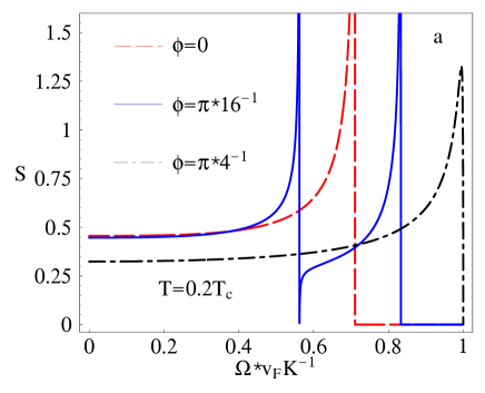
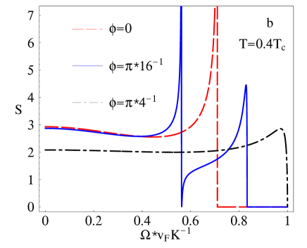
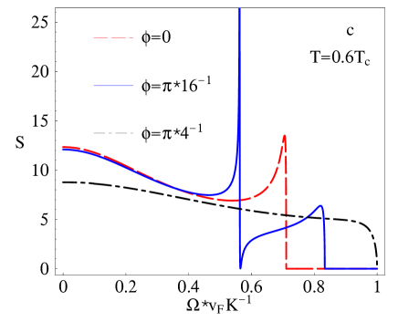
Figure 3: Structure factor $S(\Omega,\mathbf{K})$ in arbitrary units: (a) $T=0.2T_{c}$, (b) $T=0.4T_{c}$ and (c) $T=0.6T_{c}$. We put $\omega_{p}=0.5\epsilon_{F}$, $v_{F}K=0.01\epsilon_{F}$ (i.e. $v_{F}K=0.02\omega_{p}$) and $\alpha_{D}=10$, so that $T_{c}\approx 0.063\epsilon_{F}$.

In Fig. 3 (a) - (c) we show the structure factor calculated using the analytical expressions mentioned above for different temperatures. The position of the peaks defined by the ratio $\Omega/v_{F}K$ is well fitted by Eq. (53). In particular, for $\phi=\pi/16$ two peaks are seen. This allows to associate the origin of these peaks with the gap nodes. As expected the peaks are getting less sharp and higher as the temperature increases. The width of the peaks also depends on the direction of $\mathbf{K}$: for a larger value of $\phi$ ($0<\phi<\pi/4$) the corresponding peak is wider. All these results are in agreement with Fig. 3 from Takada.2000 , but due to the analytical character of the calculation the subtle peak features have a better resolution.

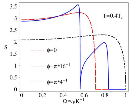
Figure 4: Structure factor $S(\Omega,\mathbf{K})$ in arbitrary units for $T=0.4T_{c}$. The rest of the parameters is the same as in Fig. 3, except for the fact that the density-current coupling is “switched off” ($\Pi_{03}^{\alpha}=0$.)

To argue that these peaks in Fig. 3 are indeed due to the density-current coupling in Fig. 4 we show for comparison the structure factor which was calculated setting $\Pi_{30}^{\alpha}=0$. The disappearance of the peaks confirms our claim that the CG mode demands nonzero density-current coupling.

This procedure of setting $\Pi_{03}^{\alpha}$ equal to zero is in fact very convenient in clarifying the origin of the peaks, because even for $\Pi_{03}^{\alpha}$ some peaks can be seen because both $\Pi_{33}$ and $\Pi_{00}^{\alpha\beta}$ have the square root singularities discussed in Sec. IV. For example, for $\pi/16<\phi<\pi/4$ (see Fig. 5) the lower peak becomes even sharper, but in contrast to to Fig. 4 it does not disappear when we set $\Pi_{03}^{\alpha}=0$.

VI.4 Manifestations of the CG mode in the classical response functions

The structure factor considered above is so important for the investigation of the CG mode because for superconductors there is no a classical laboratory field that couples, to and in the static limit is the thermodynamic conjugate of the order parameter. The reason that there is no laboratory conjugate field in the superconductor and superfluid cases is that these order parameters are off-diagonal in number space Goldman.1981 . Nevertheless it is interesting to investigate whether the CG mode can manifest itself in the “classical” correlators when one goes beyond the static limit.

Let us firstly consider the form $M_{\varphi}$ for the electric potential. Substituting the elements of the matrix Eq. (27) in Eq. (31) we arrive at the following expression (compare with Eq. (37))

$$\begin{split}\mathcal{M}_{\varphi}^{-1}(i\Omega_{n},{\bf K})=4e^{2}\left(\frac{-\Pi_{33}\Lambda^{\alpha\beta}K_{\alpha}K_{\beta}+\Pi_{03}^{\alpha}\Pi_{30}^{\beta}K_{\alpha}K_{\beta}}{-\Omega_{n}^{2}\Pi_{33}+\Lambda^{\alpha\beta}K_{\alpha}K_{\beta}-i\Omega_{n}K_{\alpha}\Pi_{03}^{\alpha}-i\Omega_{n}K_{\alpha}\Pi_{30}^{\alpha}}+V_{c}^{-1}(\mathbf{K})\right).\end{split}$$ (54)

One can verify that both plasma and CG modes are present in the equation $\mathcal{M}_{\varphi}^{-1}=0$.

Although the equation $\mathcal{M}_{\varphi}^{-1}=0$ is gauge independent, $\mathcal{M}_{\varphi}^{-1}$ itself as well as $\mathcal{M}_{\theta}^{-1}$ is gauge dependent. This time, however, we can take instead of $\mathcal{M}_{\varphi}$ truly gauge independent correlators Eq. (39). Note that the definition Eq. (39) with the source fields $(A_{0},\mathbf{A})$ clearly shows that the “classical laboratory field” is used to probe the corresponding response. Then repeating the calculation of Eqs. (41) and (42) with nonzero $\Pi_{03}^{\alpha}$ we arrive at the gauge independent density-density

$$\chi(i\Omega_{n},{\bf K})=\frac{e^{2}(\mathbf{\bar{\Pi}}_{03}^{\alpha}\mathbf{\bar{\Pi}}_{30}^{\beta}-\mathbf{\bar{\Pi}}_{33}\mathbf{\bar{\Lambda}}^{\alpha\beta})K_{\alpha}K_{\beta}}{\mathbf{\bar{\Lambda}}^{\alpha\beta}K_{\alpha}K_{\beta}-\mathbf{\bar{\Pi}}_{33}\Omega_{n}^{2}-i\Omega_{n}K_{\alpha}\mathbf{\bar{\Pi}}_{03}^{\alpha}-i\Omega_{n}K_{\alpha}\mathbf{\bar{\Pi}}_{30}^{\alpha}}.$$ (55)

and current-current

$$\chi^{\alpha\beta}(i\Omega_{n},{\bf K})=e^{2}\left(\mathbf{\bar{\Lambda}}^{\alpha\beta}-\frac{(i\Omega_{n}\mathbf{\bar{\Pi}}_{03}^{\alpha}-\mathbf{\bar{\Lambda}}^{\alpha\mu}K_{\mu})(i\Omega_{n}\mathbf{\bar{\Pi}}_{30}^{\beta}-\mathbf{\bar{\Lambda}}^{\nu\beta}K_{\nu})}{\mathbf{\bar{\Lambda}}^{\alpha\beta}K_{\alpha}K_{\beta}-\mathbf{\bar{\Pi}}_{33}\Omega_{n}^{2}-i\Omega_{n}K_{\alpha}\mathbf{\bar{\Pi}}_{03}^{\alpha}-i\Omega_{n}K_{\alpha}\mathbf{\bar{\Pi}}_{30}^{\alpha}}\right),$$ (56)

correlators.

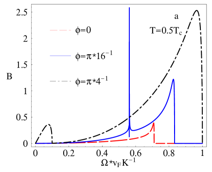
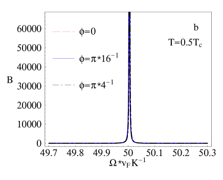
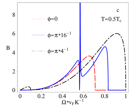
Figure 6: Spectral density $B(\Omega,\mathbf{K})$ in arbitrary units for $T=0.5T_{c}$. (a) $0\leq\Omega/v_{F}K\leq 1$ and $\Pi_{03}^{\alpha}\neq 0$, (b) $49\leq\Omega/v_{F}K\leq 51$ and $\Pi_{03}^{\alpha}\neq 0$, (c) $0\leq\Omega/v_{F}K\leq 1$ and $\Pi_{03}^{\alpha}=0$. We put $\omega_{p}=0.5\epsilon_{F}$, $v_{F}K=0.01\epsilon_{F}$ (i.e. $\omega_{p}=50v_{F}K$) and $\alpha_{D}=10$. To display the $\delta$-like plasma peak seen in Fig. 6 (b) a small imaginary part is added to $\omega_{p}$.

In Fig. 6 we show the spectral density

$$B(\Omega,\mathbf{K})=\frac{1}{\pi}\mbox{Im}\chi(\Omega,\mathbf{K})$$ (57)

calculated for the density-density correlator Eq. (55). The plasma mode (see Fig. 6 (b)) and the CG mode (see Fig. 6 (a)) as proves Fig. 6 (c) are clearly seen in the density-density correlator. We note that for $\phi=\pi/16$ the lower peak does not change strongly showing that it is due to the density-density correlations and not the CG mode.

As the value of $K$ decreases the relative weight of the CG mode with respect to the plasma mode becomes smaller and smaller as shown in Fig. 7. Finally in the limit

$$\chi(i\Omega_{n},{\bf K})\sim-\frac{e^{2}\mathbf{\bar{\Pi}}_{33}\mathbf{\bar{\Lambda}}^{\alpha\beta}K_{\alpha}K_{\beta}}{\mathbf{\bar{\Lambda}}^{\alpha\beta}K_{\alpha}K_{\beta}},\qquad\frac{\Omega}{K}=\mbox{const},\mathbf{K}\to 0,$$ (58)

the CG mode disappears from the density-density correlator. This agrees with the statement of Takada.1998 that the density-density correlator in the limit $\mathbf{K}\to 0$ is dominated by the plasma oscillation only.

Treating the current-current correlator Eq. (56) in the same way one obtains

$$\chi^{\alpha\beta}(i\Omega_{n},{\bf K})\sim e^{2}\left(\mathbf{\bar{\Lambda}}^{\alpha\beta}-\frac{\mathbf{\bar{\Lambda}}^{\alpha\mu}K_{\mu}\mathbf{\bar{\Lambda}}^{\nu\beta}K_{\nu}}{\mathbf{\bar{\Lambda}}^{\alpha\beta}K_{\alpha}K_{\beta}}\right),\qquad\frac{\Omega}{K}=\mbox{const},\Omega\to 0.$$ (59)

Taking into account that the structure of $\mathbf{\bar{\Lambda}}^{\alpha\beta}$ is $\mathbf{\bar{\Lambda}}^{\alpha\beta}=\Lambda\delta_{\alpha\beta}-Fv_{F\alpha}v_{F\beta}$ one can check that the term with $F$ cancels out from the transverse correlator. This shows that the longitudinal CG mode cannot be seen in the transverse current-current correlator and its presence does not have any influence on the Meissner effect in the limit $\mathbf{K}\to 0$.

VII Discussion

In the present paper we have shown that the 2D model of clean $d$-wave superconductor predicts the existence of the CG mode in a wide temperature region down to $T=0.1T_{c}$. This is done using the analytical expression for the structure factor which has peaks associated with the CG mode and solving numerically the equation for the CG mode velocity, $v_{CG}$. All our results are in a good agreement with the paper Takada.2000 where a similar model has been studied numerically using the formalism of Kulik.1981 . It was also shown in Takada.2000 that in contrast to $s$-wave superconductors where the impurities supressing the Landau damping result in more favourable conditions for the observation of the CG mode, in $d$-wave superconductors the CG mode disappears in the dirty system.

Thus the main physical question is whether our prediction of the CG mode in a clean $d$-wave superconductor is relevant for HTSC cuprates which are very complex compounds. Recent measurements Zhang done in high-purity YBa₂Cu₃O₇ crystals show that the in-plane mean free path $l$ increases to $\simeq 1\mu m$ below $T=20K(\approx 0.22T_{c})$. This suggests that these systems are deeply in the clean limit $l\gg\xi\sim 10\dot{A}$ ($\xi$ is the in-plane superconducting coherence length) and the model we considered can be applied to describe the CG mode in these compounds. Using the value of the Fermi velocity $v_{F}\approx 1.8\times 10^{7}cm/s$ from Zhang we predict that the velocity of the CG mode is expected to be within the range $v_{CG}=(1/\sqrt{2}\,-\,1)v_{F}\approx(1.3\,-\,1.8)\times 10^{5}m/c$ depending on the direction of $\mathbf{K}$ which is one or two orders of magnitude faster than the velocity of the CG mode observed in conventional superconductors.

From the theoretical point of view there are many questions which deserve further theoretical investigation. First of all, it would still be important to consider the influence of impurities and inelastic scattering by antiferromagnetic spin fluctuations within the proposed formalism. It is also interesting to estimate the widening of the structure factor peaks which is discussed above Eq. (18). This widening may become important if temperatures $T\lesssim T_{c}$ are considered.

The discovery of the CG mode in conventional superconductors led to much deeper understanding of superconductivity, so we hope that the investigation of the same problem in HTSC would also increase understanding of these complex systems.

VIII Acknowledgments

We gratefully acknowledge Prof. V.P. Gusynin for numerous fruitful discussions, careful reading of the manuscript and his patience in explaining us the issue of gauge invariance. We also thank Prof. A. Fetter for useful discussion and Prof. V.M. Loktev for critical remarks on the manuscript and Prof. P.Martinoli for bringing our attention to the existence of the CG mode and his constant interest to our progress. S.G.Sh. is grateful to the members of the Institut de Physique, Université de Neuchâtel for hospitality. This work was supported by the research project 2000-061901.00/1 of the Swiss National Science Foundation.

Appendix A General expressions for polarizations $\Pi_{ij}$

The general expressions for the polarization functions $\Pi_{ij}$ are (see e.g. Takada.1997 ; we.LD ; Aitchison.2000 )

$$\begin{split}&\begin{bmatrix}\Pi_{00}^{\alpha\beta}(i\Omega_{n},{\bf K})\\ \Pi_{33}(i\Omega_{n},{\bf K})\end{bmatrix}=\\ \\ &-\int\frac{d^{2}k}{(2\pi)^{2}}\left\{\frac{1}{2}\left(1-\frac{\xi_{-}\xi_{+}\pm\Delta_{-}\Delta_{+}}{E_{-}E_{+}}\right)\left[\frac{1}{E_{+}+E_{-}+i\Omega_{n}}+\frac{1}{E_{+}+E_{-}-i\Omega_{n}}\right][1-n_{F}(E_{-})-n_{F}(E_{+})]\right.\\ &\left.+\frac{1}{2}\left(1+\frac{\xi_{-}\xi_{+}\pm\Delta_{-}\Delta_{+}}{E_{-}E_{+}}\right)\left[\frac{1}{E_{+}-E_{-}+i\Omega_{n}}+\frac{1}{E_{+}-E_{-}-i\Omega_{n}}\right][n_{F}(E_{-})-n_{F}(E_{+})]\right\}V_{\pm}(\mathbf{k})\,,\\ &\qquad\qquad\qquad V_{\pm}(\mathbf{k})\equiv\begin{bmatrix}v_{F\alpha}(\mathbf{k})v_{F\beta}(\mathbf{k}),&``+^{\prime\prime};\\ 1,&``-^{\prime\prime}.\end{bmatrix}\,,\end{split}$$ (60)

and

$$\begin{split}&\Pi_{03}^{\alpha}(i\Omega_{n},{\bf K})=\\ &=\int\frac{d^{2}k}{(2\pi)^{2}}\left\{\left(\frac{\xi_{+}}{2E_{+}}-\frac{\xi_{-}}{2E_{-}}\right)\left[\frac{1}{E_{+}+E_{-}+i\Omega_{n}}-\frac{1}{E_{+}+E_{-}-i\Omega_{n}}\right][1-n_{F}(E_{-})-n_{F}(E_{+})]\right.\\ &\left.+\left(\frac{\xi_{+}}{2E_{+}}+\frac{\xi_{-}}{2E_{-}}\right)\left[\frac{1}{E_{+}-E_{-}+i\Omega_{n}}-\frac{1}{E_{+}-E_{-}-i\Omega_{n}}\right][n_{F}(E_{-})-n_{F}(E_{+})]\right\}v_{F\alpha}(\mathbf{k}),\end{split}$$ (61)

where $\xi_{\pm}\equiv\xi({\bf k}\pm{\bf K}/2)$, $E_{\pm}\equiv E({\bf k}\pm{\bf K}/2)$ and $\Delta_{\pm}\equiv\Delta({\bf k}\pm{\bf K}/2)$. One can also check that $\Pi_{30}^{\alpha}(i\Omega_{n},{\bf K})=\Pi_{03}^{\alpha}(i\Omega_{n},{\bf K})$.

The first and second terms in Eqs. (60) and (61) have a clear physical interpretation Schrieffer . The first term proportional $1-n_{F}(E_{-})-n_{F}(E_{+})$ gives the contribution from “superfluid” electrons. The second term gives the contribution of the thermally excited quasiparticles (i.e. “normal” fluid component). This is the term responsible for the appearance of the Landau terms in the effective action (see e.g. Aitchison.2000 ; we.LD ). The imaginary part of these terms is the only source of damping of the phase excitations in the clean system considered here. The physical origin of this damping is due to the scattering of the thermally excited quasiparticles from the phase excitations.

Since in what follows we are interested in the limit $\Omega,v_{F}K\ll\Delta_{0}$ we may safely neglect $\Omega$ and $K$ in the first terms of Eqs. (60), (61) and write

$$\Pi_{33}(\Omega,{\bf K})\approx-\int\frac{d^{2}k}{(2\pi)^{2}}\left\{\frac{\Delta^{2}({\bf k})}{E^{3}({\bf k})}\tanh\frac{E({\bf k})}{2T}+\frac{\xi^{2}({\bf k})}{E^{2}({\bf k})}\frac{2(E_{+}-E_{-})}{(E_{+}-E_{-})^{2}-\Omega^{2}}[n_{F}(E_{-})-n_{F}(E_{+})]\right\},$$ (62)

$$\Pi_{00}^{\alpha\beta}(\Omega,{\bf K})\approx-\int\frac{d^{2}k}{(2\pi)^{2}}\frac{2(E_{+}-E_{-})}{(E_{+}-E_{-})^{2}-\Omega^{2}}[n_{F}(E_{-})-n_{F}(E_{+})]v_{F\alpha}({\bf k})v_{F\beta}({\bf k}),$$ (63)

$$\Pi_{03}^{\alpha}(\Omega,{\bf K})\approx-\int\frac{d^{2}k}{(2\pi)^{2}}\frac{\xi({\bf k})}{E({\bf k})}\frac{2\Omega}{(E_{+}-E_{-})^{2}-\Omega^{2}}[n_{F}(E_{-})-n_{F}(E_{+})]v_{F\alpha}({\bf k}).$$ (64)

This approximation is in agreement with the one used in Appendix C of Takada.1997 .

Appendix B Nodal approximation

The key values which are necessary for evaluation of the polarizations Eqs. (62), (63) and (64) are the differences $E_{+}-E_{-}$ and $n_{F}(E_{+})-n_{F}(E_{-})$. Expanding in $\mathbf{K}$,

$$E({\bf k}+{\bf K}/2)-E({\bf k}-{\bf K}/2)=\mathbf{v}_{g}(\mathbf{k})\mathbf{K}\,,$$ (65)

where the quasiparticle group velocity is given by

$$\mathbf{v}_{g}(\mathbf{k})=\nabla_{\mathbf{k}}E(\mathbf{k})=\frac{1}{E(\mathbf{k})}\left[\xi(\mathbf{k})\mathbf{v}_{F}+\Delta(\mathbf{k})\mathbf{v}_{\Delta}\right]\,.$$ (66)

It is obvious that due to the gap $\mathbf{k}$-dependence Eq. (65) differs from the $s$-wave case Aitchison.2000 by the second term Lee . To perform the calculation analytically it is useful to rewrite Eqs. (65) and (66) in terms of the nodal approximation described in detail in Lee (see also Sec. VII of we.LD where the imaginary parts of these polarizations were calculated.) In particular, using this approximation one has $\varepsilon(\mathbf{k})\simeq p_{1}\equiv v_{F}k_{1}=p\cos\delta$, $\Delta(\mathbf{k})\simeq p_{2}\equiv v_{\Delta}k_{2}=p\sin\delta$ with $E(\mathbf{k})\simeq p=\sqrt{p_{1}^{2}+p_{2}^{2}}=\sqrt{v_{F}^{2}k_{1}^{2}+v_{\Delta}^{2}k_{2}^{2}}$, where the quasiparticle momentum $\mathbf{k}=(k_{1},k_{2})$ is written in the nodal coordinate system $\hat{\mathbf{k}}_{1}$, $\hat{\mathbf{k}}_{2}$ associated with $j$-th node ($j=1,\ldots,4$). (Note that the angle $\delta$ was denoted in Lee ; we.LD as $\varphi$). Then

$${\bf v}_{g}{\bf K}=v_{F}K_{1}\cos\delta+v_{\Delta}K_{2}\sin\delta\equiv P\cos(\delta-\psi)\,,\qquad E({\bf k}\pm{\bf K}/2)\ll\Delta_{0}\,,$$ (67)

where the momentum $\mathbf{K}=(K_{1},K_{2})$ of $\theta$-particle is also expressed in the nodal coordinate system $\hat{\mathbf{k}}_{1}$, $\hat{\mathbf{k}}_{2}$, so that $P^{1}\equiv v_{F}K_{1}=P\cos\psi$, $P^{2}\equiv v_{\Delta}K_{2}=P\sin\psi$ and $P=\sqrt{(P^{1})^{2}+(P^{2})^{2}}=\sqrt{v_{F}^{2}K_{1}^{2}+v_{\Delta}^{2}K_{2}^{2}}$. (We denoted the components of ${\bf P}$ as $P^{1},P^{2}$ to make them different from the node label $P_{j}$ used in what follows.) Finally, we can approximate the difference $n_{F}(E_{+})-n_{F}(E_{-})$ as

$$n_{F}(E_{+})-n_{F}(E_{-})\approx\frac{dn_{F}(E)}{dE}{\bf v}_{g}{\bf K}=\frac{dn_{F}(E)}{dE}P\cos(\delta-\psi).$$ (68)

Recall also that in the nodal approximation the integral over the original Brillouin zone is replaced by the integration over 4 nodal sub-zones as

$$\int\frac{d^{2}k}{(2\pi)^{2}}\to\sum_{j=1}^{4}\int\frac{dk_{1}dk_{2}}{(2\pi)^{2}}\to\sum_{j=1}^{4}\int\frac{d^{2}p}{(2\pi)^{2}v_{F}v_{\Delta}}=\sum_{j=1}^{4}\int_{0}^{p_{max}}\frac{pdp}{2\pi v_{F}v_{\Delta}}\int_{0}^{2\pi}\frac{d\varphi}{2\pi}\,,\quad p_{max}=\sqrt{\pi v_{F}v_{\Delta}}/a\,.$$ (69)

It is necessary to underline that the nodal approximation is designed for the low temperature regime $T\ll\Delta_{0}$. Thus all polarizations derived in Appendix C are applicable for $T\ll\Delta_{0}$.

Appendix C Calculation of $\Pi_{ij}$ and equation for $T_{c}$

After the substitution Eqs. (67), (68) in Eq. (62) and integration over $p$ (see we.LD ) $\Pi_{33}$ is expressed via the integral

$$I=\int_{0}^{2\pi}\frac{d\delta}{2\pi}\frac{\cos^{2}\delta\cos^{2}(\delta-\psi)}{\cos^{2}(\delta-\psi)-b^{2}}$$ (70)

with $b=|\Omega|/P_{j}$. (Note that we omitted the sub-zone index $j$ in $\psi$ and $b$.) This integral can be calculated using the table integral (3.682) from Gradshteyn for $b^{2}>1$ giving

$$I=\frac{1}{2}+b^{2}\cos 2\psi-\frac{|b|^{3}}{\sqrt{b^{2}-1}}\cos^{2}\psi+|b|\sqrt{b^{2}-1}\sin^{2}\psi\,.$$ (71)

Then using the analytical continuation in the region $b^{2}<1$, we finally arrive at the result

$$\begin{split}\Pi_{33}(\Omega,{\bf K})=&-\kappa(T)-\sum_{j=1}^{4}\frac{\ln 2}{\pi}\frac{T}{v_{F}v_{\Delta}}\left\{\frac{1}{2}+\frac{\Omega^{2}}{P_{j}^{2}}\cos 2\psi_{j}-\frac{|\Omega|}{P_{j}}\frac{1}{\sqrt{\frac{\Omega^{2}}{P_{j}^{2}}-1}}\left[\frac{\Omega^{2}}{P^{2}_{j}}\cos^{2}\psi_{j}-\left(\frac{\Omega^{2}}{P_{j}^{2}}-1\right)\sin^{2}\psi_{j}\right]\Theta\left(\frac{|\Omega|}{P_{j}}-1\right)\right.\\ +&\left.i\frac{\Omega}{P_{j}}\frac{1}{\sqrt{1-\frac{\Omega^{2}}{P_{j}^{2}}}}\left[\frac{\Omega^{2}}{P_{j}^{2}}\cos^{2}\psi_{j}+\left(1-\frac{\Omega^{2}}{P_{j}^{2}}\right)\sin^{2}\psi_{j}\right]\Theta\left(1-\frac{|\Omega|}{P_{j}}\right)\right\},\end{split}$$ (72)

where $\kappa(T)$ denotes the term which originates from the first term in the braces of Eq. (62) which cannot be accurately calculated using the nodal approximation we.LD . It is easy to show, however, that $\kappa=m/\pi$ at $T=0$ for the continuum $s$-wave pairing model. This can be used to write $\Pi_{33}$ in the dimensionless form:

$$\Pi_{33}(\Omega,{\bf K})=\frac{m}{\pi}{\tilde{\Pi}}_{33}(\Omega,{\bf K}),$$ (73)

where

$${\tilde{\Pi}}_{33}(\Omega,{\bf K})=-{\tilde{\kappa}}-\sum_{j=1}^{4}\frac{\ln 2}{2}\frac{T}{\epsilon_{F}}\alpha_{D}\left\{\cdots\right\},$$ (74)

where $\cdots$ are the terms in the braces in Eq. (72), $\epsilon_{F}=mv_{F}^{2}/2$ is the Fermi energy, $\alpha_{D}=v_{F}/v_{\Delta}$ (see Sec. II) and we assume that ${\tilde{\kappa}}\sim 1$. One can also check that the imaginary part of $\Pi_{33}$ coincides with the expression calculated in we.LD integrating $\delta(P\cos(\delta-\psi)-\Omega)$.

In the same way we arrive at the expression for the current-current polarization function Eq. (63):

$$\Pi_{00}^{\alpha\beta}(\Omega,{\bf K})K_{\alpha}K_{\beta}/K^{2}=-\sum_{j=1}^{4}\frac{\ln 2}{\pi}\frac{T}{v_{F}v_{\Delta}}\frac{P_{j}^{2}\cos^{2}\psi_{j}}{K^{2}}\left[1-\frac{|\Omega|}{P_{j}}\frac{1}{\sqrt{\frac{\Omega^{2}}{P_{j}^{2}}-1}}\Theta\left(\frac{|\Omega|}{P_{j}}-1\right)+i\frac{\Omega}{P_{j}}\frac{1}{\sqrt{1-\frac{\Omega^{2}}{P_{j}^{2}}}}\Theta\left(1-\frac{|\Omega|}{P_{j}}\right).\right]$$ (75)

The zero order superfluid stiffness $\Lambda_{0}^{\alpha\beta}=\delta_{\alpha\beta}n/m$ for the continuum ($m_{\alpha\beta}(\mathbf{k})=m\delta_{\alpha\beta}$) system at $T=0$, where $n$ is the total carrier density which, of course, coincides with the density of the neutralizing background. Using the expression $\epsilon_{F}=\pi n/m$ which is, strictly speaking, valid only for the 2D systems with the quadratic dispersion law, we can also rewrite the superfluid stiffness $\Lambda_{\alpha\beta}$ in the dimensionless form

$$\Lambda^{\alpha\beta}(\Omega,\mathbf{K})\frac{K_{\alpha}K_{\beta}}{K^{2}}\equiv\frac{\epsilon_{F}}{\pi}{\tilde{\Lambda}}=\frac{\epsilon_{F}}{\pi}\left[{\tilde{\Lambda}_{0}}-\sum_{j=1}^{4}\ln 2\frac{T}{\epsilon_{F}}\alpha_{D}\frac{P_{j}^{2}}{(v_{F}K)^{2}}\cos^{2}\psi_{j}\cdots\right]\,.$$ (76)

As was already mentioned after Eq. (72), the terms which contain the averaging over the Fermi surface (see e.g. Eqs. (24) and (25)) cannot be accurately calculated using the nodal approximation we.LD . Thus, in general ${\tilde{\Lambda}_{0}}$ as well as ${\tilde{\kappa}}$ should be considered as a free parameter of the model. In particular, decreasing the value of ${\tilde{\Lambda}_{0}}$ it is possible to describe a lowering of the zero temperature superfluid stiffness in HTSC. Nevertheless, for the numerical computations we will assume that ${\tilde{\Lambda}_{0}}\sim 1$. It is easy to obtain (see e.g. Lee ; we.LD ) that the static, zero momentum bare superfluid stiffness

$$\Lambda=\frac{\epsilon_{F}}{\pi}\left({\tilde{\Lambda}_{0}}-2\ln 2\alpha_{D}\frac{T}{\epsilon_{F}}\right)$$ (77)

and that the velocity of the BA mode

$$v=\sqrt{\frac{\Lambda}{\Pi_{33}(0,\mathbf{K})}}=\frac{v_{F}}{\sqrt{2}}\sqrt{\frac{{\tilde{\Lambda}_{0}}-2\ln 2\alpha_{D}T/\epsilon_{F}}{{\tilde{\kappa}}}}\,.$$ (78)

so that for ${\tilde{\Lambda}_{0}}={\tilde{\kappa}}=1$ the BA mode velocity $v(T=0)=v_{F}/\sqrt{2}$. Using Eq. (77) one can estimate the temperature of Berezinskii-Kosterlitz-Thouless transition from the equation $T_{c}=\pi/2\Lambda(T_{c})$, which gives

$$T_{c}=\frac{\epsilon_{F}{\tilde{\Lambda}_{0}}}{2(1+\ln 2\alpha_{D})}.$$ (79)

We will use this definition of $T_{c}$ to express the temperature $T$ in the units of $T_{c}$ and $\epsilon_{F}$.

Finally, we obtain that the expression for Eq. (64)

$$\Pi_{03}^{\alpha}(\Omega,{\bf K})K_{\alpha}/K=-\sum_{j=1}^{4}\frac{T}{\pi v_{F}}\left\{\alpha_{D}\ln 2\frac{\Omega}{v_{F}K}\cos\psi_{j}\left[\cos\psi_{j}-\frac{|\Omega|}{P_{j}}\frac{\cos\psi_{j}}{\sqrt{\frac{\Omega^{2}}{P_{j}^{2}}-1}}\Theta\left(\frac{|\Omega|}{P_{j}}-1\right)+i\frac{\Omega}{P_{j}}\frac{\cos\psi_{j}}{\sqrt{1-\frac{\Omega^{2}}{P_{j}^{2}}}}\Theta\left(1-\frac{|\Omega|}{P_{j}}\right)\right]\right\}\,,$$ (80)

where we put inside the braces the dimensionless part, ${\tilde{\Pi}_{03}}^{\alpha}K_{\alpha}/K$.

Appendix D Equations for $v_{CG}$, structure factor and transformation to the global coordinate system

Substituting Eqs. (73), (76) and (80) in Eq. (46), we obtain the equation for CG mode in the dimensionless form which is convenient for numerical investigation

$${\tilde{\Lambda}}=\frac{T^{2}}{2\epsilon_{F}^{2}}\frac{({\tilde{\Pi}_{03}}^{\alpha}K_{\alpha}/K)^{2}}{{\tilde{\Pi}_{33}}}\,.$$ (81)

The whole expression (44) for $M_{\theta}^{-1}$ can also be written as

$$M_{\theta}^{-1}(\Omega,\mathbf{K})=\frac{m}{\pi}v_{F}^{2}K^{2}{\tilde{M}}_{\theta}^{-1}(\Omega,\mathbf{K}),$$ (82)

where

$${\tilde{M}}_{\theta}^{-1}(\Omega,\mathbf{K})=\frac{\Omega^{2}}{v_{F}^{2}K^{2}}\mathbf{\hat{\Pi}}_{33}(\Omega,\mathbf{K})-\frac{\Omega}{v_{F}K}\mathbf{\hat{\Pi}}_{03}^{\alpha}(\Omega,\mathbf{K})\frac{K_{\alpha}}{K}+\frac{1}{2}\mathbf{\hat{\Lambda}}^{\alpha\beta}\frac{K_{\alpha}K_{\beta}}{K^{2}},$$ (83)

where the dimensionless polarization functions $\mathbf{\hat{\Pi}}_{33}$, $\mathbf{\hat{\Pi}}_{03}^{\alpha}$ and $\mathbf{\hat{\Lambda}}^{\alpha\beta}$ were made from the full polarization functions $\mathbf{\bar{\Pi}}_{33}$, $\mathbf{\bar{\Pi}}_{03}^{\alpha}$, $\mathbf{\bar{\Lambda}}^{\alpha\beta}$ (see Eqs. (33) and (44)) in the same way as the polarizations Eqs. (73), (76) and (80). The only difference is that these full polarizations include the Coulomb potential $V_{c}(\mathbf{K})$ (for simplicity we take the 3D potential) which for our purposes is convenient to rewrite as

$$V_{c}^{-1}(\mathbf{K})=\frac{m}{2\pi}\frac{v_{F}^{2}K^{2}}{\omega_{p}^{2}}\,,$$ (84)

where $\omega_{p}$ is the plasma frequency defined after Eq. (36).

Although the local nodal coordinate systems $(P_{j},\psi_{j})$ are very convenient for calculating of the polarization functions Eqs. (74), (76) and (80), the final expressions for them and, for example, Eq. (82) have to be calculated in the global or laboratory coordinate system $(K,\phi)$. It is convenient to measure the angle $\phi$ from the vector $\hat{k}_{x}$, so that $\phi=0$ corresponds to the corner of the Fermi surface (see e.g. Fig. 1 in we.LD ) and the first node is at $\phi=\pi/4$. Thus the transformations from the global coordinate system into the local system related to the $j$-th node are

$$\begin{split}&P_{j}=K\sqrt{v_{F}^{2}\cos^{2}\left(\phi-\frac{\pi}{4}+\frac{\pi}{2}(j-1)\right)+v_{\Delta}^{2}\sin^{2}\left(\phi-\frac{\pi}{4}+\frac{\pi}{2}(j-1)\right)}\,,\\ &\cos\psi_{j}=\frac{v_{F}K}{P_{j}}\cos\left(\phi-\frac{\pi}{4}+\frac{\pi}{2}(j-1)\right)\,,\qquad\sin\psi_{j}=\frac{v_{\Delta}K}{P_{j}}\sin\left(\phi-\frac{\pi}{4}+\frac{\pi}{2}(j-1)\right)\,,\qquad j=1,\ldots,4.\end{split}$$ (85)

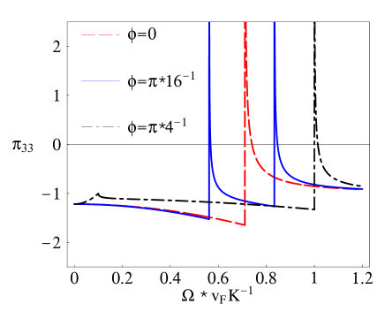
Figure 1: Real part of $\Pi_{33}(\Omega,\mathbf{K})$ (or more precisely ${\tilde{\Pi}}_{33}(\Omega,\mathbf{K})=(\pi/m)\Pi_{33}(\Omega,\mathbf{K})$, see Eq. (74)). We put $T=0.5T_{c}$ ($T_{c}$ and the angle $\phi$ are defined in Appendices C and D, respectively) and $\alpha_{D}=10$.

References

- (1) R.V. Carlson, A.M. Goldman, Phys. Rev. Lett. 34, 11 (1975).
- (2) F.E. Aspen, A.M. Goldman, J. Low Temp. Phys. 43, 559 (1981).
- (3) N.N. Bogolyubov, V.V. Tolmachev,D.N. Shirkov, A new method in the theory of superconductivity, (Consultants Bureau, New York, 1959.)
- (4) P.W. Anderson, Phys. Rev. B 110, 827 (1958); 112, 1900 (1958).
- (5) S.N. Artemenko, A.F. Volkov, Usp. Fiz. Nauk. 128, 3 (1979) [Sov. Phys.Usp. 22, 295 (1979)].
- (6) J. Clarke, A. Schmid, C. J.Pethick and H. Smith, A.M. Goldman in Nonequilibrium Superconductivity, Phonons, and Kapitza Boundaries, edited by K.E. Gray (NATO ASI Series, Plenum, New York, 1981), Chaps. 13,14,15,17.
- (7) E.V. Bezuglij, E.N. Bratus’, V.P. Galaiko, J. Low Temp. Phys. 47, 511 (1982).
- (8) J. Clarke, J. Beyer et al., A.M. Kadin and A.M. Goldman, A.G.Aronov et al., V.M. Galitskii et al., G. Schön in Nonequilibrium Superconductivity, edited by D.N. Langenberg and A.I. Larkin (Elsevier, Amsterdam, 1986), Chaps. 1,4,7,8,9,13.
- (9) I.O. Kulik, Ora Entin-Wohlman, R. Orbach, J. Low Temp. Phys. 43, 591 (1981).
- (10) K.Y.M. Wong, S. Takada, Phys. Rev. B 37, 5644 (1988).
- (11) Y. Ohashi, S. Takada, J. Phys. Soc. Jpn. 66, 2437 (1997).
- (12) Y. Ohashi, S. Takada, Phys. Rev. B 62, 5971 (2000).
- (13) S.N. Artemenko, A.G. Kobelkov, Phys. Rev. B 55, 9094 (1997).
- (14) S.N. Artemenko, S.V. Remizov, Phys. Rev. Lett. 86, 708 (2001).
- (15) C.C. Tsuei, J.R. Kirtley, Rev. Mod. Phys. 72, 969 (2000).
- (16) V.M. Loktev, R.M. Quick and S.G. Sharapov, Phys. Rep. 349, 1 (2001).
- (17) A. Paramekanti, M. Randeria, T.V. Ramakrishnan, S.S. Mandal, Phys. Rev. B 62, 6786 (2000).
- (18) S.G. Sharapov, H. Beck, V.M. Loktev, Phys. Rev. B 64, 134519 (2001).
- (19) L. Benfatto, A. Toschi, S. Caprara, C. Castellani, Phys. Rev. B. 64, 140506 (2001).
- (20) A.A. Varlamov, V.V. Dorin, Zh. Eksp. Teor. Fiz. 91, 1955 (1986) [Sov. Phys. JETP 64, 1159 (1986)].
- (21) R.A. Smith, M.Yu. Reizer, J.W. Wilkins, Phys. Rev. B 51, 6470 (1995).
- (22) R.A. Smith, V. Ambegaokar, Phys. Rev. B 62, 5913 (2000).
- (23) Y. Ohashi, S. Takada, J. Phys. Soc. Jpn. 67, 551 (1998).
- (24) I.J.R. Aitchison, G. Metikas, D.J. Lee, Phys. Rev. B 62, 6638 (2000).
- (25) N. Nagaosa, Quantum Field Theory in Condensed Matter Physics, Springer-Verlag, Berlin, 1999.
- (26) M. Capezzali, D. Ariosa, H. Beck, Physica B 230-232, 962 (1997).
- (27) H. Kleinert, Fortschritte der Physik 26, 565 (1978).
- (28) “Low energy” means that the energy of the phase distortions is smaller than than the enery gain, due to the gap opening for neutral or for charged system Randeria.action .
- (29) Since we are interested in the regime when the free vortex excitations are absent, it is safe to use the symmetric form of this transformation, O. Vafek, A. Melikyan, M. Franz, Z. Tesǎnović, Phys. Rev. B 63, 134509 (2001).
- (30) For completness we reintroduced for a moment the Planck’s constant . Note also that in the conventions that we used the charge of electron is
- (31) H.J. Mikeska, Sol. St. Comm. 13, 73 (1973).
- (32) F. Weling, A. Griffin, M. Carrington, Phys. Rev. B 28, 5296 (1983).
- (33) A.M. Tsvelik, Quantum Field Theory in Condensed Matter Physics, Cambridge University Press, 1995. Chap. 12.
- (34) L. Benfatto, S. Caprara, C. Castellani, A. Paramekanti, M. Randeria, Phys. Rev. B 63, 174513 (2001).
- (35) V.P. Gusynin, I.A. Shovkovy, Phys. Rev. D 64, 116005 (2001); Nucl. Phys. A 700, 403 (2002).
- (36) I.J.R. Aitchison, C.M. Fraser, Ann. Phys. (N.Y.) 156, 1 (1984).
- (37) J.R. Schrieffer, Theory of Superconductivity, Benjamin, New York, 1964.
- (38) A. Schmid, G. Schön, Phys. Rev. Lett. 34, 941 (1975).
- (39) This is, of course, applied to 3D, not 2D superconductor. However, to study HTSC the influence of the third direction has to be taken into account as done, for example, in Takada.2000 .
- (40) In principle, a more general equation (34) without taking its real part has to be studied to extract the information about the damping of the CG mode, but this significantly increases the difficulty of the numerical work. From this point of view a direct computation of the structure factor which does not demand solving any equation is more straightforward.
- (41) Y. Zhang, N.P. Ong, P.W. Anderson, D.A. Bonn, R. Liang, W.N. Hardy, Phys. Rev. Lett. 86, 890 (2001).
- (42) A.C. Durst, P.A. Lee, Phys. Rev. B 62, 1270 (2000).
- (43) I.S. Gradshteyn, I.M. Ryzhik, Table of Integrals, Series and Products (Academic Press, New York, 1980).