Charge and spin ordering, and charge transport properties in a two-dimensional inhomogeneous $t-J$ model

Abstract

We study a two-dimensional $t-J$ model close to the Ising limit in which charge inhomogeneity is stabilized by an on-site potential $e_{s}$, by using diagonalization in a restricted Hilbert space and finite temperature Quantum Monte Carlo. Both site and bond centered stripes are considered and their similitudes and differences are analyzed. The amplitude of charge inhomogeneity is studied as $e_{s}\rightarrow 0$. Moreover, we show that the anti-phase domain ordering occurs at a much lower temperature than the formation of charge inhomogeneities and charge localization. Hole-hole correlations indicate a metallic behavior of the stripes with no signs of hole attraction. Kinetic energies and current susceptibilities are computed and indications of charge localization are discussed. The study of the doping dependence in the range $0.083\leq x\leq 0.167$ suggests that these features are characteristic of the whole underdoped region.

PACS: 71.10.Fd, 74.80.-g, 74.72.-h

]

I Introduction

After many years of intensive research the physics of underdoped high-T_c cuprates is still far from being wholly understood. This underdoped region, where strongly correlated electron effects are most important, are considered by many to contain the key to explain central features of these materials, including the superconducting phase. One of the main features of the underdoped cuprates is the presence of the pseudogap which has been intensely studied with several experimental techniques.[1, 2] In spite of this intense effort, there is still not a clear picture of the origin of the pseudogap and its relation with the superconducting gap.[3] Another interesting phenomena observed by experiments in some underdoped cuprates is the presence of ordered charge inhomogeneities (“stripes”) followed (as the temperature is decreased) by the appearance of incommensurate (IC) magnetic correlations.[4, 5, 6] These charge inhomogeneities provide a natural explanation for the pseudogap. There is also strong experimental evidence of the presence of charge ordering/stripes in other transition metal oxides like manganites and nickelates.[7, 8] Again, in spite of an enormous amount of research, there is not yet a clear picture of the mechanism leading to stripe formation and the relation between stripes and superconductivity in the cuprates. Different and in many cases competing scenarios have been proposed to explain these issues.[9, 10, 11, 12]

From the theoretical point of view, in addition to the conceptual complexity of strongly correlated electron systems, there are important methodological difficulties. In stripes theories, phenomenological models of coupled Luttinger (or Luther-Emery) liquids have been studied[13] providing useful insight in the problem although quantitative estimations are usually lacking. In any case, these phenomenological models have to be supported by the study of models at a more microscopic level. These microscopic models (variants of Hubbard, $t-J$ models) are most frequently studied by numerical methods which also have to deal with severe limitations (some of them will be discussed in Section II). It is then absolutely necessary to complement different approaches and to contrast the results obtained by analytical and numerical techniques in order to get a consistent picture of the physics of underdoped cuprates.

In this article a model of stripes is studied by numerical techniques. The model is defined as a two-dimensional (2D) $t-J$ model where stripes are stabilized by an effective on-site potential representing the effect of extrinsic features to Cu-O planes like lattice anisotropy,[14] effect of chains in YBa₂Cu₃O_7-δ (Ref. [6]) or other structural details, Coulomb interaction due to off-plane charges, electron-phonon coupling,[12] etc. This model has been studied numerically on small clusters ($4\times 4$) at both zero[15, 16] and finite temperatures.[17]. Results on larger clusters with periodic boundary conditions were obtained in Ref. [18], although at the price of working close to the Ising limit of the Heisenberg term of the Hamiltonian. In the present article we present an exhaustive analysis of this model by using quantum Monte Carlo (QMC) techniques, in particular, we examine the behavior at various doping and the effects of the anisotropy of the exchange term of the Hamiltonian. These analysis at finite temperature are complemented with zero temperature studies with a diagonalization technique in a reduced Hilbert space known as “systematically expanded Hilbert space” (SEHS).[19] The results obtained with both QMC and SEHS allow a comparison not only with experiment but also with previous calculations on similar clusters but with (partially) open boundary conditions.[10, 20]

The paper is organized as follows. In Section II, the model considered is defined and some elementary details of the techniques employed are discussed. In Section III we present results obtained with QMC and SEHS for the stripe filling as a function of the on-site potential both for site- and bond-centered stripes (defined in Section II). In Section IV we study charge and spin ordering as a function of temperature and in Section V we show the behavior of the kinetic energy and current susceptibility with temperature as an indication of charge transport properties in the underdoped region. Finally, in the Conclusions we summarize the results as an unified picture of the evolution of the various physical quantities examined as a function of temperature.

II Model and methods.

The Hamiltonian of the $t-J$ model with an anisotropic exchange term is:

$$H_{tJ}= - t\sum_{\langle{ij}\rangle,\sigma}({\tilde{c}}^{\dagger}_{i\sigma}{\tilde{c}}_{j\sigma}+h.c.)$$ (1)

$$+ J\sum_{\langle{ij}\rangle}(\frac{\gamma}{2}(S^{+}_{i}S^{-}_{j}+S^{-}_{i}S^{+}_{j})+S^{z}_{i}S^{z}_{j}-{\frac{1}{4}}n_{i}n_{j})$$ (2)

where the notation is standard. $i,j$ are sites on a square lattice. $N$ site clusters with fully periodic boundary conditions (PBC) were considered. We adopted $t=1$ as the unit of energy and temperature and $J=0.35$. In some cases we considered $J=0.7$, specially because it reduces the sign problem. $\gamma=0$ corresponds to the Ising limit or $t-J_{z}$ model.[21] The stripes are stabilized by an effective on-site potential:

$$H_{str}=\sum_{i}{e_{s}}_{i}n_{i}$$ (3)

On “site centered” (SC) stripes ${e_{s}}_{i}=-e_{s}<0$ on equally spaced vertical columns, as in the original picture of Ref. [4], and ${e_{s}}_{i}=e_{s}$ on the remainder sites. At each doping fraction, the number of stripes imposed is such that the linear hole density on the stripes at infinite potential is 1/2. We shall come to this point later on this section.

The QMC method employed is an implementation of the usual world-line algorithm with the checkerboard decomposition[22, 18]. The “minus sign” problem[23] becomes more severe as lattice size and doping are increased and temperature is decreased. It is absent if holes are confined to move in one dimension and the XY tern in the Heisenberg interaction is set to zero. The behavior of the average sign as a function of various parameters of the model is shown in Fig. 1 of Ref. [18]. We checked our code against for the $4\times 4$ cluster with one site-centered stripe, 2 holes, $J/t=0.35$, $e_{s}=1$. We extrapolated our results to zero temperature and compared them against the ones obtained with Lanczos exact diagonalization. The relative error for the energy was of the order of $10^{-4}$, and for correlations $10^{-3}$. For larger clusters, smaller $e_{s}$, or larger $\gamma$ the correlation’s error estimated from different independent runs may be as large as 10 $\%$ at the lowest temperature attainable. In general, we kept $\Delta=\beta/M=0.083$, where $\beta=1/T$ and $M$ is the Trotter number. For the lowest temperatures of our simulations ($T/t\approx 0.1$) the measurement runs were as long as 1.6 10⁶ MC sweeps. With these very long simulations we were able to deal with $\langle sgn\rangle$ as small as 0.05. On the largest clusters we considered, $8\times 8$ and $12\times 12$, we studied $e_{s}\approx 2$, which corresponds to well-defined charge inhomogeneities (see next section), and has been also taken in previous related studies.[15, 16]

SEHS is a zero temperature diagonalization in a Hilbert space that is expanded by successive hole hoppings, starting from an initial state (e.g. holes on the stripes). After each expansion the Hamiltonian is diagonalized with the Lanczos algorithm and a fraction of the most weighted configurations of the ground state is kept for the next iteration.[19] The goal is that after several back and forth steps, an optimal set of states is selected for a given dimension of the Hilbert space. The Hilbert space is grown to a maximum dimension (determined of course by the computational resources available) and finally the quantities of interest are extrapolated to the full dimension of the Hilbert space of the system. In many cases reliable qualitative behaviors are obtained without this final extrapolation. The whole procedure is variational but it shares many of the virtues of exact diagonalization like the possibility of computing any physical quantity both static and dynamical. Another advantage that SEHS shares with Lanczos diagonalization is the possibility of working for a given set of quantum numbers, in particular since periodic boundary conditions can be used, it is possible to work at a given momentum. In addition there are no constraints on the model studied. In the following section we will apply this technique to the $t-J_{z}$ model but in principle it could be applied to the isotropic exchange although in this case requirements of time and memory are much larger. Another possibility offered by this technique is that long-range Coulomb interactions can be handled, as a difference with QMC. We will explore in the future this possibility.

The use of the on-site potential to stabilize stripes could be thought as leading to “static” stripes, not in the sense of “pinned” (since we are working with periodic boundary conditions) but in the sense of suppressing stripe fluctuations. The opposite meaning of “static” could be applied to the stripes resulting from density matrix renormalization group (DMRG) calculations[10] with open boundary conditions along the longer direction of the cluster. In this case, it is well known that “bond-centered” (BC) stripes are obtained rather than SC ones. This fact may reflect the also well known tendency of holes to form pairs in the 2D $t-J$ model at zero temperature.[24] However, SC stripes are much sharper features than BC stripes and they seem more consistent with elastic neutron scattering, NQR and ARPES[25] data at low doping although not definite conclusions can be drawn yet. At higher doping there have been speculations that more BC stripes may be formed at the expense of SC stripes thus explaining some experimental features.[26]

III Stripe filling.

Our first study concerns the evolution of charge inhomogeneity as a function of the applied on-site potential in the 2D $t-J_{z}$ model. Zero temperature results were obtained with SEHS for a $8\times 4$ cluster, 4 holes (hole doping fraction $x=1/8$), PBC. Stripes were imposed along the shorter direction ($y$ axis). Translations along both directions, reflection along an horizontal axis and spin reversal symmetries were imposed and the dimension of the Hilbert space was grown up to $\approx 8.6~{}10^{6}$. The ground state in the case of SC stripes corresponds to $(q_{x},q_{y})=(0,\pi)$ and to $(0,0)$ in the BC case.

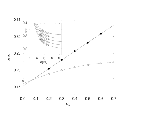
FIG. 1.: Hole density on stripe sites on the $8\times 4$ cluster, $J/t=0.35$, as a function of the on-site potential $e_{s}$. Circles (triangles) correspond to SC (BC) stripes. Solid and dashed lines are quadratic extrapolations to $e_{s}=0$. The star indicates the result obtained with DMRG[27] for (almost) BC stripes on the same system but mixed boundary conditions. The inset shows the stripe densities as a function of the dimension of the Hilbert space and their extrapolation to the full dimension. From bottom to top $e_{s}=0.2,\ldots,0.6$.

Results for the stripe filling are depicted in Fig. 1 for $J/t=0.35$ as a function of the on-site potential. Details of the extrapolation to the full Hilbert space dimension for each $e_{s}$ with a power law are shown in the inset of this figure. These densities are then extrapolated with a quadratic polynomial to $e_{s}=0$. The final extrapolated values of the stripe densities are very similar (0.153 for SC and 0.159 for BC stripes) and they are quite close to those obtained with DMRG in Refs. [10, 20]. Of course the linear density in the BC case would correspond to the double of that quantity, but this concept is somewhat misleading because it hides its relative smoothness with respect to SC stripes. It has been also previously shown that the effect of exchange anisotropy is not very important.[20] We also include for comparison the DMRG result for the same model, cluster and parameters but using mixed boundary conditions (open (periodic) along the direction perpendicular (parallel) to the stripes).[27] In this case, the occupancy of the two legs on a stripe is slightly different and their average value was taken. As expected, the open boundary conditions along the direction transversal to the stripes leads to a somewhat larger charge inhomogeneity than our results with fully PBC.

FIG. 2.: Hole density on stripe sites on the $8\times 4$ and $8\times 8$ clusters, $J/t=0.35$, as a function of the on-site potential $e_{s}$ favoring a SC stripe. The dashed line corresponds to the uniform doping $x=1/8$. Points above this line correspond to the stripe; below it, they correspond to the first column next to the stripe. Solid lines are quadratic fitting to the data.

In the case of SC stripes we can compare the previous results with the ones obtained with QMC. The temperature dependence of the stripe density is very smooth[18] and it has been extrapolated to zero temperature with a power law. The stripe hole density on the $8\times 4$ cluster obtained with QMC is shown in Fig. 2. The resulting error of the finite temperature data and of the extrapolation procedure can be appreciated from the dispersion of the data. Nevertheless, the overall agreement between QMC results and the ones obtained with SEHS is certainly very good. The results for a larger cluster, $8\times 8$, are quite consistent with the previous ones. The stripe density seems somewhat smaller than for $8\times 4$, which could be explained by the geometric anisotropy of this cluster making it more “one-dimensional” thus favoring the formation of a charge density wave along the long axis. However, error bars can likely mask this effect, if it exists.

From the results of Fig. 2 one can also infer that to have a stripe filling close to $1/2$, let us say, larger than 0.4, the effective on-site potential should be $\approx 1$ in the case of SC stripes, and somewhat smaller ($\approx 0.35$) in the case of BC stripes. Then, a sizable on-site potential, specially in the case of SC stripes is necessary to stabilize this charge inhomogeneity. A possible mechanism, not included explicitly in our model, an in-plane long range Coulomb repulsion,[9] could help to reduce the requirement of an external agent in order to make stripes stable. A long-range potential cannot be implemented in the world-line QMC used here (it cannot be implemented in DMRG calculations either) but it could be included in the SEHS scheme as we noticed in the previous section.

IV Charge and spin ordering.

There is now mounting experimental evidence that spin ordering, signalled by incommensurate (IC) peaks in the magnetic structure factor, follows charge ordering as temperature decreases.[4, 28, 29] That is, charge degrees of freedom are the driving force of stripe formation. Similar behavior occurs in stripe formation in nickelates[8] and manganites.[7] In the model here considered, in spite of a sizable charge inhomogeneity at high temperatures, IC magnetic structure appears at much lower temperatures in agreement with experiment. This is a nontrivial result, since some theoretical models of stripe formation do not properly account for this ordering sequence.[20, 11]

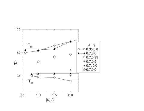
FIG. 3.: Phase diagram in the temperature-on-site potential plane obtained for the $8\times 8$ cluster, $x=1/8$. $T_{CO}$ and $T_{SO}$ correspond to the crossovers in the charge and spin sectors discussed in the text. The point indicated with a star was obtained on the $12\times 12$ cluster, $x=0.083$). Diamonds indicate the temperature at which the inverse kinetic energy along to the stripes are minimum.

As an introduction to this section, we reproduce the phase diagram in the temperature-e_s plane obtained in our previous work[18] for SC stripes (Fig. 3). By measuring charge and spin static structure factors ($C({\bf k})$ and $S({\bf k})$, respectively), two crossovers have been determined. At high temperature there is a crossover in the charge sector determined by a change in the peak of $C({\bf k})$ from $(0,0)$ to $(2\delta,0)$ ($\delta=2x\pi$). At a much lower temperature, there is a crossover in the spin sector signalled by the peak of $S({\bf k})$ splitting from $(\pi,\pi)$ to $(\pi\pm\delta,\pi)$, which correspond to the peaks seen in neutron scattering experiments. Between these two crossovers, typical temperature or energy scales related to transport properties are located, as we will discuss in Section V. These temperature scales have been adopted to experimentally determine the onset of the pseudogap.[2]

The change of the peak in $C({\bf k})$ in our model is just a consequence of stripe formation: $(2\delta,0)$ corresponds to the main Fourier component of a pure SC stripe (away from $(0,0)$). The change of the peak in $S({\bf k})$ corresponds to the formation of anti-phase domains,[4] a feature which is reproduced in our model.[18] In the following subsections we will more systematically study the effect of the anisotropy in the exchange term of the Hamiltonian and the doping dependence of the results for SC stripes. In the last subsection, we report similar studies for BC stripes.

A Effect of the XY term.

Although an antiferromagnetic (AF) correlation in the direction perpendicular to the Cu-O planes would imply as a second order process an effective exchange anisotropy in the plane, it is clear that the most interesting model to study is the one that involves an isotropic (or nearly isotropic) Heisenberg term. Unfortunately, a more isotropic exchange implies stronger minus sign problem and hence, we are limited to consider $\gamma\leq 0.5$. However, as we show below, one can get an insight on how and to what extent a more isotropic coupling changes the results obtained on the Ising limit.

Let us consider the hole-hole and spin-spin correlations defined by

$$C({\bf i,j})=\langle n_{\bf i}n_{\bf j}\rangle$$ (4)

and

$$S({\bf i,j})=\langle S^{z}_{\bf i}S^{z}_{\bf j}\rangle$$ (5)

respectively. $n_{\bf i}$ is the hole occupation number at site ${\bf i}$; ${\bf i}=(x,y)$ and ${\bf j}=(x^{\prime},y^{\prime})$. In particular, if a SC stripe along $y$ is located at $x=x_{s}$, we are interested in the correlations along the stripe, where ${\bf i}=(x_{s},0)$, ${\bf j}=(x_{s},r)$, and in correlations across the stripe, corresponding to ${\bf i}=(x_{s}-a,y)$, ${\bf j}=(x_{s}+a,y)$ (the inset of Fig. 4 shows the case of $a=1$).

In Fig. 4, the spin-spin correlation across a vertical stripe (indicated with filled circles in the inset) is shown for the $8\times 8$ cluster, $x=1/8$, $J=0.7$, $e_{s}=1.5$, and $\gamma=0$, 0.25, and 0.5. These correlations show the change

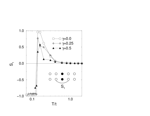
FIG. 4.: Spin-spin correlation across the stripe (shown in the inset) on the $8\times 8$ cluster, $x=1/8$, $J=0.7$, $e_{s}=1.5$, and several values of the XY term $\gamma$.

of sign corresponding of the spin domains going from in-phase to anti-phase at the magnetic crossover temperature. Their amplitude decrease as expected with increasing $\gamma$ but the crossover temperature remains roughly unaffected. In this, and in in similar figures, typical error bars are about the size of the largest symbols used.

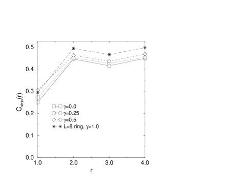
FIG. 5.: Hole-hole correlations along the stripe on the $8\times 8$ cluster, $x=1/8$, $J=0.7$, $e_{s}=1.5$, and several values of the XY term $\gamma$. Results obtained by exact diagonalization on the quarter filled 8-site ring at zero temperature are also shown for comparison.

Another important result of Ref. [18], viz. the metallic behavior of the hole-hole correlations along a stripe is also quite robust against the increase of the XY term of the exchange interaction. In Fig. 5, we show these correlations for the $8\times 8$ cluster, $x=1/8$, $J=0.7$, $e_{s}=1.5$, and $\gamma=0$, 0.25, and 0.5 extrapolated to zero temperature. It can be seen that their behavior remains unchanged with $\gamma$ except for a uniform shift, within error bars (of the order of the symbol size). This shift corresponds to a larger filling of the stripe as $\gamma$ increases.

B Doping dependence.

The study of the dependence of the results with doping is essential to determine the extent to which the present mode is physically realistic. For this study, we performed QMC simulations on the $12\times 12$ cluster, with 12 holes ($x=0.083$) and 24 holes ($x=0.167$). In the first case, two SC stripes six lattice spacings apart were stabilized by an on-site potential, and in the second case four SC stripes three lattice spacings apart. We have in addition results for the $8\times 8$ cluster with eight holes and for the $12\times 12$ cluster with 18 holes both corresponding to $x=0.125$. In the latter cluster, care should be taken because the three SC stripes present imply that the three intervening spin regions cannot be in anti-phase.

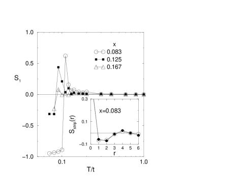
FIG. 6.: Spin-spin correlations on the $12\times 12$ cluster, $x=1/8$, $J=0.35$, $e_{s}=2.0$, $\gamma=0$, at several dopings indicated on the text. The inset shows the spin-spin correlation along the stripe vs. distance (open circles) at $T=0.09$ compared with exact results on a quarter filled 12 sites chain (filled circles) at the same temperature.

The spin-spin correlations across the stripe are shown in Fig. 6. The amplitude of the magnetic order both above and below the crossover temperature decreases with doping and so it does the crossover temperature itself, which is in agreement with experiments. At $x=0.125$, for the $8\times 8$ cluster, the crossover temperature is larger than that for the $12\times 12$ one (due to the frustration mentioned above), but smaller than the corresponding at $x=0.083$ (see Fig. 3). The inset shows $S(r)$ along the stripe for the same parameters, at the lowest reachable temperature ($T=0.09$), and the corresponding results for a chain obtained by exact diagonalization at the same temperature, showing a remarkable agreement between them.

The hole-hole correlations along a stripe, extrapolated to zero temperature, are shown in Fig. 7 for the same parameters as in Fig. 6. These correlations also present the $4k_{F}$ oscillation of a quarter-filled chain seen in Fig. 4 with no signs of hole attraction. This behavior, together with the above mentioned similarity of spin-spin correlations indicate that SC stripes behave at low temperatures like an isolated chain.

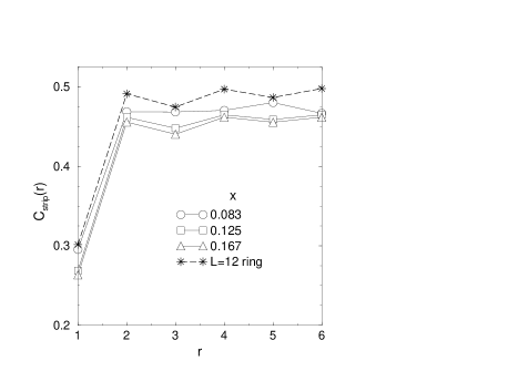
FIG. 7.: Hole-hole correlations along a stripe on the $12\times 12$ cluster, $x=1/8$, $J=0.35$, $e_{s}=2.0$, $\gamma=0$. Results obtained by exact diagonalization on the 12 site chain at zero temperature are also shown for comparison.

C Bond-centered stripes.

Bond centered stripes are stabilized by applying ${e_{s}}_{i}=-e_{s}<0$ on equally spaced stripes consisting of two nearest neighbor columns and ${e_{s}}_{i}=e_{s}>0$ otherwise. In this case, the sign problem, which is much worst than for SC stripes, imposes us further limitations on the accessible parameters and temperatures. Hence, this study was done for the $8\times 8$ cluster at $x=1/8$ filling and on the Ising limit of the Hamiltonian.

If the stripe legs along the $y$ direction are located at $x=x_{s}$ and $x_{s}+1$, then the correlations across the stripe involve the sites ${\bf i}=(x_{s}-1,y)$, ${\bf j}=(x_{s}+2,y)$. The rung correlations relate the sites ${\bf i}=(x_{s},y)$, ${\bf j}=(x_{s}+1,y)$. The correlations along the stripes may correspond to the same leg (${\bf i}=(x_{s},0)$, ${\bf j}=(x_{s},r)$) or to opposite legs (${\bf i}=(x_{s},0)$, ${\bf j}=(x_{s}+1,r)$).

Our first important result is related to the appearance of anti-phase spin ordering of the intervening domains at a temperature at which the charges are already essentially moving on the stripes, in complete analogy to what happens for SC stripes and in contrast with some speculations based on an spin-only model.[30] This result can be inferred from the spin-spin correlations shown in Fig. 8, obtained for $J=0.7$, $e_{s}=1.5$, $\gamma=0$. For $J=0.35$, $e_{s}\leq 2$, the sign problem inhibits us to reach low enough temperatures. The variation of stripe filling with temperature, also included in this Figure, shows that its zero temperature value is mostly achieved already at $T\approx t$. The spin-spin correlation across the stripe ($S_{1}$) experiences a sign change, in this case from AF to ferromagnetic, at $T\approx 0.15t$, after it reaches its maximum AF value which occurs in turn once spin order in the intervening spin ladders (as shown along the legs at the maximum distance, $S_{2}$, and on the rungs, $S_{3}$), is well established. In fact, the inter-domain correlation $S_{1}$ starts to vary with temperature at a much lower temperature than the intra-domain ones, $S_{2}$ and $S_{3}$. The spin correlation on stripe rungs ($S_{4}$) essentially vanishes below the crossover temperature. These combined features suggest that, at least for the parameters examined, the formation of anti-phase domain is a result of a collective interplay between spin domains and not a result of local correlations on the stripes.

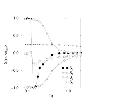
FIG. 8.: Spin-spin correlations on the $8\times 8$ cluster, $x=1/8$, $J=0.7$, $e_{s}=1.5$, $\gamma=0$, with bond centered stripes. $S_{i},i=1,\ldots,4$ are defined in the text. The hole density on the stripe, $<n_{str}>$ is shown with crosses.

On the other hand, the peak in the charge structure factor at $(\pi/4,0)$ remains unchanged down from $T\approx 5$ for the same parameters of Fig. 4. At larger temperatures $C({\bf k})$ is virtually constant at nonzero momentum.

Let us examine next hole-hole correlations. In Fig. 9 we show these correlations, for the same parameters as before, as a function of distance at the lowest temperature available. We have also included for comparison the exact correlations obtained for a $2\times 8$ quarter-filled ladder at $T=0$, with the same parameters and various values of $\gamma$. Two features are apparent. First, for $\gamma=0$, correlations on the stripe are quite different from their zero temperature, isolated ladder, counterparts. In the inset of this Figure, it is shown that the temperature evolution of the stripe correlations is quite smooth down to the lowest temperature reached. This behavior suggests that BC stripes do not behave like isolated ladders unless there is some other crossover at lower temperatures. Second, notice that in isolated ladders pairing occurs near the isotropic limit of the exchange interaction ($\gamma\geq 0.5$) of the $t-J$ model. Unfortunately, it is not possible to reach low enough temperatures and large values of $\gamma$ with our QMC algorithm to further investigate these issues.

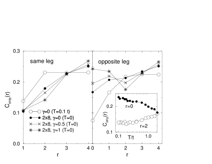
FIG. 9.: Hole-hole correlations on the $8\times 8$ cluster, $x=1/8$, $J=0.7$, $e_{s}=1.5$, $\gamma=0$. Results obtained by exact diagonalization on the $2\times 8$ cluster at zero temperature are also shown for comparison.

V Charge transport.

Another important issue a theory of stripes should address is the behavior of resistivity in the underdoped region. Resistivity measurements on high-quality La_2-xSr_xCuO₄ (LSCO) and YBa₂Cu₃O_y single crystals[31] show a metallic behavior at moderate temperatures in a wide range of doping. These experiments also show a divergent resistivity as $T\rightarrow 0$ which was earlier detected in LSCO (Ref. [32]) and in Bi₂Sr_2-xLa_xCuO_6+δ (Ref. [33]) even after suppressing superconductivity with magnetic fields. The inverse mobility of carriers, also shown in Ref. [32], has a similar behavior with temperature as the resistivity.

A measure of charge mobility is the kinetic energy, which can be easily computed in QMC and it is affected by relatively small errors. In addition, the kinetic energy, due to the use of PBC, is the most important contribution to the Drude weight (defined below). Although a straightforward comparison with the above mentioned experimental results is not possible, one can get some interesting qualitative insights in the problem.

Further information on charge transport properties can be gained by looking at the “paramagnetic” contribution to the Drude weight.[34] To this end, we computed the current-current correlations in imaginary time defined as:

$$C_{\alpha\alpha}(\tau)=\langle j_{\alpha}(\tau)j_{\alpha}\rangle=\sum_{l,m}\langle j_{\alpha,l}(\tau)j_{\alpha,m}\rangle$$ (6)

$$=\sum_{l,m}\frac{1}{\cal Z}Tr\{j_{\alpha,l}(\tau)j_{\alpha,m}e^{-\beta H}\}$$ (7)

where the paramagnetic ${\bf q}=(0,0)$ current operator along direction $\alpha$ ($\alpha={\hat{x}},{\hat{y}}$) is:

$$j_{\alpha}=\sum_{l}j_{\alpha,l}=it\sum_{l,\sigma}({\tilde{c}}^{\dagger}_{l+\alpha,\sigma}{\tilde{c}}_{l,\sigma}-{\tilde{c}}^{\dagger}_{l,\sigma}{\tilde{c}}_{l+\alpha,\sigma})$$ (8)

and $j_{\alpha,l}(\tau)=e^{\tau H}j_{\alpha,l}e^{-\tau H}$, $\tau=l\Delta$, $0\leq l<M$. ${\cal Z}=Tr\{e^{-\beta H}\}$ is the partition function. Since $j_{\alpha,l}$ conserves particle number and spin the calculation of $\langle j_{\alpha,l}(\tau)j_{\alpha,m}\rangle$ is relatively simple. Since,

$$\langle j_{\alpha}(\tau)j_{\alpha}\rangle=\frac{1}{\pi}\int_{-\infty}^{\infty}\frac{\omega{\sigma^{\prime}_{\alpha}}_{reg}(\omega)}{1-e^{-\beta\omega}}e^{-\tau\omega}d\omega$$ (9)

where ${\sigma^{\prime}_{\alpha}}_{reg}(\omega)$ is the regular part of the real part of the conductivity along the $\alpha$-direction, it can be shown that:

$$\chi_{\alpha}=\int_{0}^{\beta}\langle j_{\alpha}(\tau)j_{\alpha}\rangle d\tau=\frac{2}{\pi}\int_{0}^{\infty}{\sigma^{\prime}_{\alpha}}_{reg}(\omega)d\omega$$ (10)

Then, from the standard f-sum rule one obtains the expression for the Drude weight:[34]

$$\frac{2D_{\alpha}}{\pi}=-\chi_{\alpha}+\frac{1}{N}\langle K_{\alpha}\rangle$$ (11)

More elaborated analysis, such as the study of the dependence of the conductivity with frequency, imply the analytical continuation of imaginary time current-current correlations to real frequencies by, for instance, the maximum entropy method. This procedure is no longer in principle exact and results would be affected with large error bars.

Let us first examine the inverse kinetic energy per site as a function of temperature and for various doping fractions in the case of site centered stripes. In Fig. 10 we show the results of QMC simulations for the inverse kinetic energy per site along and perpendicular to the stripes, $\kappa_{y}=(K_{y}/N)^{-1}$ and $\kappa_{x}=(K_{x}/N)^{-1}$ resp., on the $12\times 12$ cluster, $J=0.35$, $e_{s}=2.0$, for the $t-J_{z}$ model, and fillings $x=0.083$, 0.125, and 0.167. Both quantities decrease with doping, following the general trend as the inverse mobilities in Ref. [32]. Most interestingly, it can be seen that although $\kappa_{y}$ has a positive slope in the whole temperature range, consistent with a metallic behavior of the stripes and in agreement with the results obtained in the previous section, $\kappa_{x}$ changes it sign from positive slope at high temperature to negative at low temperature indicating charge localization in the direction perpendicular to the stripes.

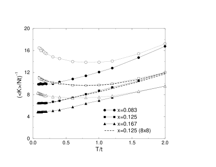
FIG. 10.: Inverse kinetic energy per site along (filled symbols) and perpendicular (open symbols) to the stripes on the $12\times 12$ cluster, $J=0.35$, $e_{s}=2.0$, and $\gamma=0.0$. Different dopings are indicated on the plot. Dashed line corresponds to results obtained on the $8\times 8$ cluster.

One can determine a temperature scale where $\kappa_{x}$ and $\kappa_{y}$ start to separate (within error bars) from each other as $T$ is lowered. This temperature scale coincides roughly with $T_{CO}$ in Fig. 3. Another scale, at a lower temperature, can be determined at the minimum of $\kappa_{x}$, i.e. at the point where charges start to be localized in the direction transversal to the stripes. This scale of temperature, determined on the $8\times 8$ cluster as a function of $e_{s}$ has been plotted in Fig. 3. From Fig. 10, this temperature scale decreases with doping, following the general behavior of the pseudogap. This temperature scale is located between $T_{CO}$ and $T_{SO}$ in Fig. 3.

As expected, the effect of the anisotropy in the exchange term of the Hamiltonian is very small for $\kappa_{x}$ and $\kappa_{y}$. For $\gamma=0$ and 0.5, results practically coincide within error bars. On the other hand, it is instructive to compare the behavior for SC and BC stripes. In Fig. 11, we show the inverse kinetic energies obtained for the $8\times 8$ cluster, $J=0.7$, $e_{s}=2.0$, $\gamma=0$, for both types of stripes. These results show a larger mobility both along and transversal to the stripes and an absence of localization in the case of BC stripes down to the lowest temperature reached ($T=0.2t$).

The behavior of the current susceptibility $\chi_{\alpha}$ is very similar to the kinetic energy per site along the same direction. Typical results are shown in Fig. 12 obtained on the $8\times 8$ cluster for $x=0.125$, $J=0.35$, $e_{s}=2.0$, $\gamma=0$.

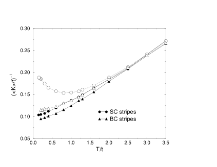
FIG. 11.: Inverse kinetic energy per site along (filled symbols) and perpendicular (open symbols) to the stripes on the $8\times 8$ cluster, $J=0.7$, $e_{s}=2.0$, $\gamma=0$ for site centered and bond centered stripes.

Two differences between those two quantities are apparent. First, the separation between the kinetic energies parallel and perpendicular to the stripes are larger than for the corresponding $\chi_{y}$ and $\chi_{x}$. Second, both temperature scales discussed above are larger for the kinetic energy per site than for the current susceptibility. Both features, which we have seen in all cases examined, suggest that the diamagnetic response is more sensitive to charge inhomogeneity than the paramagnetic one. Notice also that finite size effects for these current susceptibilities are very small.

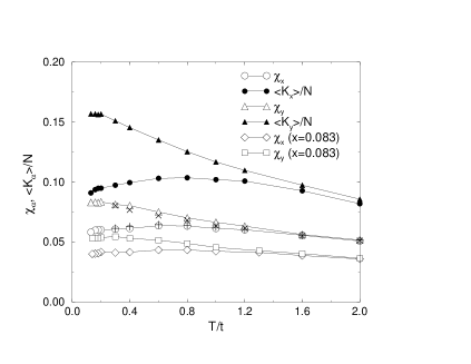
FIG. 12.: Current susceptibility and kinetic energy per site along and perpendicular to the stripes on the $8\times 8$ cluster, $x=0.125$, $J=0.35$, $e_{s}=2.0$, $\gamma=0$ for site centered stripes. $\chi_{x}$ and $\chi_{y}$ on the $12\times 12$ cluster and for the same doping are indicated with “$+$” and “$\times$” respectively. $\chi_{x}$ and $\chi_{y}$ on the $12\times 12$ cluster for $x=0.083$ are also shown.

VI Conclusions

We have examined various properties of a two-dimensional $t-J$ model in which charge inhomogeneity is stabilized by an on-site potential by using two different numerical techniques. Diagonalization in a restricted Hilbert space and finite temperature Quantum Monte Carlo techniques allow us to work with relatively large clusters with fully periodic boundary conditions. Extrapolation to the full Hilbert space and extrapolation to zero temperature give quite consistent results.

In the first place, we obtained that the linear filling in BC stripes is larger than in SC stripes. In this latter case, definitely, a stabilizing mechanism is needed if this model has to reproduce experimental results.

Then, we showed that the effect of a moderate XY term in the Heisenberg interaction does not affect the main conclusions obtained in the Ising limit in Ref. [18] for SC stripes. First, the anti-phase domain ordering, which generates the IC peaks measured in neutron scattering experiments occurs at a much lower temperature than the formation of charge inhomogeneities and charge localization. This magnetic ordering is a consequence of a collective interplay between the spin domains and are not driven by local correlations located on the stripes. Second, hole-hole correlations indicate a metallic behavior of the stripes with no signs of hole attraction. The study of the doping dependence in the range $0.083\leq x\leq 0.167$ suggest that these features are characteristic of the whole underdoped region.

In addition, we showed that some of the main conclusions for SC stripes apply to BC stripes as well, although in this case our study was mostly limited to the Ising limit of the Hamiltonian. Again, as the temperature decreases the sequence of events are: first, the formation of charge inhomogeneities, then the establishment of AF order in the intervening spin domains and finally the $\pi$-shifted magnetic ordering of the whole system. The hole-hole correlations on the stripe show again a metallic behavior and, as a difference with SC stripes, which are very similar to isolated chains, they indicate that, at finite temperatures, stripes do not behave quite like isolated ladders, unless another crossover occurs at lower temperatures than the ones we can reach.

Finally, the study of charge transport properties provides further support to the physical validity of the model defined by Eqs. (2)-(3). In particular, in the case of site centered stripes, we have shown distinctive behavior of the inverse kinetic energy, as a measure of charge mobility, in the directions parallel and perpendicular to the stripes, in this latter case showing a characteristic feature of localization. A similar behavior is observed in the paramagnetic part of the Drude weight computed through the current-current correlations. In the case of bond centered stripes, on the other hand, the increase of the inverse kinetic energy as $T\rightarrow 0$ has not been observed down to the lowest attainable temperature. Although these results were obtained near the Ising limit and for well-defined charge inhomogeneities, we believe they could help to experimentally decide between SC and BC stripes in underdoped cuprates.

- [1] T. Timusk and B. Statt, Rep. Prog. Phys. 62, 61 (1999), and references therein.
- [2] J. L. Tallon and J. W. Loram, Physica C 349, 53 (2001), and references therein.
- [3] V. M. Krasnov, A. Yurgens, D. Winkler, P. Delsing, and T. Claeson, Phys. Rev. Lett. 84, 5860 (2000).
- [4] J. M. Tranquada, B. J. Sternlieb, J. D. Axe, Y. Nakamura, and S. Uchida, Nature 375, 561 (1995); J. M. Tranquada, J. D. Axe, N. Ichikawa, Y. Nakamura, S. Uchida, and B. Nachumi, Phys. Rev. B 54, 7489 (1996); K. Yamada, C. H. Lee, K. Kurahashi, J. Wada, S. Wakimoto, S. Ueki, H. Kimura, Y. Endoh, S. Hosoya, G. Shirane, R. J. Birgeneau, M. Greven, M. A. Kastner, and Y. J. Kim , Phys. Rev. B 57, 6165 (1998).
- [5] N. Ichikawa, S. Uchida, J. M. Tranquada, T. Niemoller, P. M. Gehring, S.-H. Lee, and J. R. Schneider, Phys. Rev. Lett. 85, 1738 (2000), and references therein.
- [6] H. A. Mook, P. Dai, F. Dogan, and R. D. Hunt, Nature 404, 729 (2000).
- [7] C. H. Chen and S-W. Cheong, Phys. Rev. Lett. 76, 4042 (1996).
- [8] J. M. Tranquada, P. Wochner, A. R. Moodenbaugh, and D. J. Buttrey, Phys. Rev. B 55, 6113 (1997); P. Wochner, J. M. Tranquada, D. J. Buttrey, and V. Sachan, Phys. Rev. B 57, 1066 (1998).
- [9] V. J. Emery, S. A. Kivelson, and O. Zachar, Phys. Rev. B 56, 6120 (1997), and references therein.
- [10] S. R. White and D. J. Scalapino, Phys. Rev. B 61, 6320 (2000); Phys. Rev. B 60, 753 (1999).
- [11] J. Zaanen, O. Y. Osman, H. V. Kruis, Z. Nussinov, and J. Tworzydlo, cond-mat/0102103, and references therein.
- [12] A. H. Castro Neto, Phys. Rev. B 64, 104509 (2001).
- [13] E. W. Carlson, D. Orgad, S. A. Kivelson, and V. J. Emery, Phys. Rev. B 62, 3422 (2000); W. V. Liu and E. Fradkin, Phys. Rev. Lett. 86 1865 (2001).
- [14] This possibility has been studied in B. Normand and A. P. Kampf, Phys. Rev. B 64, 024521 (2001); A. P. Kampf, D. J. Scalapino, and S. R. White, Phys. Rev. B 64, 052509 (2001).
- [15] J. Eroles, G. Ortiz, A.V. Balatsky, and A.R. Bishop, Europhys. Lett. 50, 540 (2000).
- [16] P. Prelovsek, T. Tohyama, and S. Maekawa, Phys. Rev. B 64, 052512 (2001).
- [17] Y. Shibata, T. Tohyama, and S. Maekawa, Phys. Rev. B 64, 054519 (2001).
- [18] J. A. Riera, Phys. Rev. B 64, 104520 (2001).
- [19] José Riera, in High Performance Computing and its Applications in the Physical Sciences, edited by D. Browne, et al., (World Scientific, New York, 1994), pg. 72.
- [20] G. B. Martins, C. Gazza, and E. Dagotto, Phys. Rev. B 62, 13926 (2000).
- [21] J. Riera, and E. Dagotto, Phys. Rev. B 47, 15346 (1993); P. Prelovsek and I. Sega, Phys. Rev. B 49, 15241 (1994); A. L. Chernyshev and P. W. Leung, Phys. Rev. B 60, 1592 (1999).
- [22] J. D. Reger and A. P. Young, Phys. Rev. B 37, 5978 (1988), and references therein.
- [23] See e.g., S. Chandrasekharan and U.-J. Wiese Phys. Rev. Lett. 83, 3116 (1999), and references therein.
- [24] J. A. Riera, and A. P. Young, Phys. Rev. B 39, 9697 (1989).
- [25] X. J. Zhou, P. Bogdanov, S. A. Kellar, T. Noda, H. Eisaki, S. Uchida, Z. Hussain, and Z.-X. Shen, Science 286, 268 (1999).
- [26] X. J. Zhou, T. Yoshida, S. A. Kellar, P. V. Bogdanov, E. D. Lu, A. Lanzara, M. Nakamura, T. Noda, T. Kakeshita, H. Eisaki, S. Uchida, A. Fujimori, Z. Hussain, and Z.-X. Shen, Phys. Rev. Lett. 86, 5578 (2001).
- [27] C. J. Gazza, private communcation.
- [28] M. Fujita, H. Goka, K. Yamada, and M. Matsuda, cond-mat/0107355.
- [29] A. W. Hunt, P. M. Singer, K. R. Thurber, and T. Imai, Phys. Rev. Lett. 82, 4300 (1999).
- [30] J. Tworzydlo, O. Y. Osman, C. N. A. van Duin, and J. Zaanen, Phys. Rev. B 59, 115 (1999).
- [31] Y. Ando, A. N. Lavrov, S. Komiya, K. Segawa, X. F. Sun, Phys. Rev. Lett. 87, 017001 (2001).
- [32] Y. Ando, G. S. Boebinger, A. Passner, T. Kimura, and K. Kishio, Phys. Rev. Lett. 75, 4662 (1995).
- [33] S. Ono, Y. Ando, T. Murayama, F. F. Balakirev, J. B. Betts, and G. S. Boebinger, Phys. Rev. Lett. 85, 638 (2000).
- [34] J. Wagner, W. Hanke, and D. J. Scalapino, Phys. Rev. B 43, 10517 (1991); D. J. Scalapino, S. R. White, and S. Zhang, Phys. Rev. B 47, 7995 (1993).