The Fractional Quantum Hall effect in an array of quantum wires

Abstract

We demonstrate the emergence of the quantum Hall (QH) hierarchy in a 2D model of coupled quantum wires in a perpendicular magnetic field. At commensurate values of the magnetic field, the system can develop instabilities to appropriate inter-wire electron hopping processes that drive the system into a variety of QH states. Some of the QH states are not included in the Haldane-Halperin hierarchy. In addition, we find operators allowed at any field that lead to novel crystals of Laughlin quasiparticles. We demonstrate that any QH state is the groundstate of a Hamiltonian that we explicitly construct.

PACS numbers: 71.10.Pm, 73.43.-f, 73.43.Cd, 71.27.+a

The rich phenomenology of the quantum Hall (QH) effect provides a fertile setting for the study of correlated electrons[1]. While the integer QH effect can be understood in terms of the Landau quantization of non interacting electrons, the fractional QH state is a strongly correlated quantum liquid, where electron-electron interactions play an essential role. Motivated by Laughlin’s original variational wavefunction[2], a number of techniques have been developed to describe the hierarchy of fractional QH states[3], including composite fermion variational wavefunctions[4] and Chern-Simons field theories based on bosons[5, 6] or fermions[7]. These have lead to a deep understanding of the excitation spectrum of QH states and of the structure of the QH hierarchy.

The purpose of this paper is to develop a new formalism, which reproduces the QH hierarchy in a model consisting of a two-dimensional array of quantum wires in a perpendicular magnetic field $B$. The model could be relevant for semiconductor quantum wires, ropes of carbon nanotubes, and for stripes that arise in QH systems in the higher Landau systems [8]. Aside from the direct relevance of the model, our calculations provide a novel, and in many ways a simpler, approach to describe the fractional QH effect. Given its success in treating the Fractional QH effect, it is likely that our technique will prove useful for understanding other strongly correlated states.

We use the bosonization technique [9], developed for one-dimensional systems, and relate the QH effect to coupled Luttinger liquids. It has been shown recently [10, 11, 12] that for a range of interwire charge and current interactions, there is a phase in which interwire Josephson, charge- and spin-density-wave, and single-particle couplings are irrelevant. This sliding Luttinger liquid (SLL) or smectic metal phase is the quantum analog of the sliding phase found recently in DNA-lipid complexes and stacked XY models [13, 14]. The SLL resembles a Luttinger liquid, with transport properties that exhibit power-law singularities as a function of temperature. It has also been demonstrated [15] that in a magnetic field the phase space of SLL expands considerably.

We will show that at commensurate magnetic fields the SLL phase can be unstable to inter-wire electron hopping processes that lead the formation of an energy gap and the QH effect. The presence of the $\nu=1$ QH state in such a model was first noted by Sondhi and Yang[15]. Our calculation builds on this work. We systematically classify all electron hopping operators and identify those that lead to QH states. This construction leads to QH states which are not in the Haldane-Halperin hierarchy[3]. We also show that any QH state is the groundstate of a Hamiltonian that we explicitly construct.

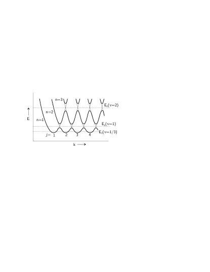
FIG. 1.: A schematic diagram showing how the Landau levels, denoted by the solid curves, arise due to coupling between neighboring single-wire bands.

We begin with a simple model of spinless electrons that ignores both electron-electron interactions and tunneling between the wires. In the Landau gauge $A=-By\hat{x}$, the electronic dispersion has the simple form,

$$E_{j}(k)={\hbar^{2}\over{2m}}(k-bj)^{2},$$ (1)

where the integer $j$ labels the wires, $b=eaB/\hbar c$, and $a$ is the separation between neighboring wires. This dispersion is characterized by level crossings, where the bands associated with different wires intersect. Tunneling between the wires couples the bands, leading to anticrossings, as indicated in Fig. 1. The Fermi energy, $E_{F}$, will lie in one of these gaps when the filling factor $\nu=2k_{F}/b$ is an integer (here $k_{F}=\pi n_{e}$ depends on the 1D electron density $n_{e}$ on each wire). In general, the gap at $E_{F}$ for $\nu=N$ results from tunneling between $N$’th neighbor wires. At these fillings, we have the analog of filled Landau levels and the integer QH effect. It can further be observed in Fig. 1 that each filled Landau level has a corresponding branch of gapless edge states.

Away from integer filling fractions the non-interacting theory has gapless excitations on each wire and corresponds to a trivial SLL fixed point. It should be noted that the near $E_{F}$ the dispersion (1) is equivalent to what would be expected in a mean field theory of QH stripes[16]. The only difference is that the left and right moving states at $E_{F}$ are no longer localized on the same wire, but rather are spatially separated. Thus, in addition to arrays of quantum wires what follows may also describe instabilities of stripe phases.

With interactions, the SLL fixed point is quite delicate, and one usually expects instabilities at low energies. To characterize the resulting phases we bosonize the states near $E_{F}$ and write [9]

$${\psi}_{R/L,j}(x)={1\over\sqrt{4\pi\epsilon}}{\eta}_{R/L,j}e^{i(bj\pm k_{F})x}e^{i\Phi_{R/L,j}(x)},$$ (2)

where $\epsilon$ is an inter-wire cut off and $\eta$ is the Klein factor. The bosonic fields $\Phi_{R/L,j}$ are related to the right and left moving electron density on each wire, $n_{R/L,j}=\pm\partial_{x}\Phi_{R/L,j}/2\pi$, which satisfy the current algebra, $[n_{R/L,j}(x),n_{R/L,j^{\prime}}(x^{\prime})]=\pm i\partial_{x}\delta(x-x^{\prime})\delta_{jj^{\prime}}/2\pi$.

The non interacting model has the Hamiltonian density ${\cal H}_{0}=\pi v_{F}\sum_{j}(n_{L,j}(x)^{2}+n_{R,j}(x)^{2})$, where $v_{F}$ is the Fermi velocity. There are two classes of interactions: forward scattering, and interchannel scattering. The forward scattering terms involve interactions between the densities of the various channels, leading to a Hamiltonian which is quadratic in the densities,

$${\cal H}_{f.s.}={\bf n}_{i}(x)^{T}{\bf M}_{ij}{\bf n}_{j}(x)$$ (3)

where ${\bf n}_{i}^{T}=(n_{R,i},n_{L,i})$ and ${\bf M}_{ij}$ is a 2 by 2 matrix. ${\cal H}_{0}+{\cal H}_{f.s.}$ describes a general SLL fixed point. To address the the instabilities of this fixed point, we consider interchannel scattering interactions. The allowed terms are built from products of single-electron operators, and may be classified according to the number of times each electron operator appears:

$${\cal O}_{\{s_{p}^{L},s_{p}^{R}\}}=\sum_{j}\prod_{p}(\psi_{R,j+p})^{s^{R}_{p}}(\psi_{L,j+p})^{s^{L}_{p}},$$ (4)

where $s_{p}^{L},s_{p}^{R}$ are integers and $\psi^{s}$ is taken to mean $(\psi^{\dagger})^{|s|}$ for $s<0$. Charge conservation requires $\sum_{p}[s_{p}^{R}+s_{p}^{L}]=0$, while momentum conservation requires

$$k_{F}\sum_{p}(s_{p}^{R}-s_{p}^{L})+b\sum_{p}p(s_{p}^{R}+s_{p}^{L})=0.$$ (5)

Operators violating (5) will upon bosonizing using (2) have an oscillating phase that renders it irrelevant at long distances.

The SLL fixed point is unstable if any allowed interchannel scattering interactions are relevant under the renormalization group. This happens when the scaling dimension $\Delta_{\{s_{p}^{R},s_{p}^{L}\}}<2$. We then expect the system to flow to a phase which is characterized by ${\cal O}_{\{s_{p}^{R},s_{p}^{L}\}}$. $\Delta_{\{s_{p}^{R},s_{p}^{L}\}}$ depends on the forward scattering interactions ${\bf M}_{ij}$. In principle, ${\bf M}_{ij}$ can be parameterized with a suitable model of the electron electron interactions. However, ${\bf M}_{ij}$ may be strongly renormalized by irrelevant and/or momentum non-conserving operators, and it may not resemble the bare interactions. Below we argue that it is usually possible to construct a Hamiltonian in which a given operator $\cal O$ is the leading relevant operator. Our approach is, therefore, to assume that $\cal O$ is relevant. We then analyze the resulting strong-coupling phase.

Symmetry requires operators related by $180^{\circ}$ rotation to be equivalent. We refer to operators which are invariant under $180^{\circ}$ rotation as “non-degenerate”. Upon bosonization these interactions have the form ${\cal H}_{\rm int}=-\sum_{i}u\cos\Xi_{i}$, where $u$ is the magnitude of the interaction and $\Xi_{i}=\sum_{p}(s_{p}^{R}\Phi_{i+p}^{R}+s_{p}^{L}\Phi_{i+p}^{L})$. For large $u$ this will tend to lock $\Xi_{i}$. Since non-degenerate operators satisfy $s_{p}^{L}=\pm s_{-p}^{R}$ it follows that $[\Xi_{i},\Xi_{j}]=0$ for all $i,j$. Thus all $\Xi_{i}$ can be simultaneously localized, and the strong coupling phase may be described by replacing $-u\cos\Xi_{i}$ by $u\Xi_{i}^{2}/2$. The Hamiltonian is then quadratic in the boson fields and the low energy excitation spectrum can be determined. Lower-symmetry “Degenerate” operators must come in pairs. An example is the single electron tunneling term $\sum_{i}[\cos(\Phi_{R,i}-\Phi_{R,i+1})+\cos(\Phi_{L,i}-\Phi_{R,i+1})]$, which leads to a 2D Fermi liquid at $B=0$. This interaction cannot be analyzed by replacing the cosine by a square because the arguments of the cosines do not commute, so localization is forbidden by the uncertainty principle. We confine our attention here to non-degenerate operators, which can be analyzed using bosonization.

The phases described by non-degenerate operators at finite $B$ fall into two general categories[17]:

(i) Crystalline states: From (5) it can be seen that when both $\sum_{p}s_{p}^{R}=\sum_{p}s_{p}^{L}=0$ and $\sum_{p}p(s_{p}^{R}+s_{p}^{L})=0$, the operator ${\cal O}_{\{s_{R},s_{L}\}}$ is allowed for any $B$. These operators, which independently conserve the number of right moving and left moving electrons lead to crystalline phases of the electrons. A simple example is the charge density wave (CDW) operator $\sum_{i}\cos[2(\theta_{i}-\theta_{i+1})]$, where $\theta_{i}=(\Phi_{R,i}-\Phi_{L,i})/2$ is the CDW phase on each wire. When this operator, depicted in Fig. 2b, dominates, the CDW’s on neighboring wires lock together forming a two dimensional Wigner crystal. It can be seen by expanding the cosine that this state has a gapless phonon mode associated with the broken translational symmetry. This category also includes more exotic crystals, such as the Abrikosov flux lattice[18] (Fig. 2e) and crystals of Laughlin quasiparticles (Fig. 2f). These states share the common feature that they are allowed at any $B$ and possess a gapless phonon mode.

(ii) Quantum Hall states: When $\sum_{p}s_{p}^{R}\neq\sum_{p}s_{p}^{L}$ the operator ${\cal O}_{\{s_{R},s_{L}\}}$ is allowed only at a special magnetic field which corresponds to filling factor

$$\nu=2{{\sum_{p}p(s_{p}^{R}+s_{p}^{L})}\over{\sum_{p}(s_{p}^{L}-s_{p}^{R})}}.$$ (6)

The denominator of (6) counts the net number of electrons backscattered from right to left moving channels. The numerator gives the change in the “center of mass” of the electrons. By replacing the cosine by a square, it can be established that these states have a gap to bulk excitations and have gapless edge states. The simplest example is the $\nu=1$ QH state described by the operator $\sum_{j}\cos[\Phi_{R,j}-\Phi_{L,j+1}]$ (Fig. 2c). This locks the right and left moving modes of neighboring wires, opening a gap for all modes except for the edge mode $\Phi_{L,1}$, which remains uncoupled. This is equivalent to the description in terms of non interacting electrons shown in Fig. 1.

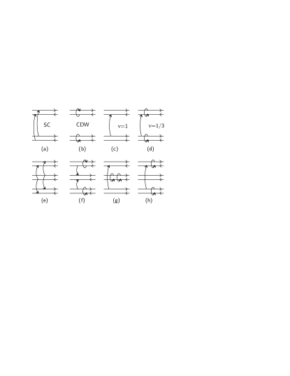
FIG. 2.: Pictorial representation of tunneling operators corresponding to the following states: (a) Superconductor, (b) CDW, (c) $\nu=1$ QH state, (d) $\nu=1/3$ QH state, (e) Abrikosov flux lattice, (f) Crystal of $\nu=1/3$ Laughlin quasiparticles, (g,h) Two distinct $\nu=2/3$ QH states.

In addition to the integer QH states, which have “single particle” energy gaps, there are a variety of fractional QH states whose gaps arise from correlated tunneling processes. The simplest correspond to the Laughlin sequence at $\nu=1/m$, where $m$ is an odd integer, and are shown in Fig. 2d for $\nu=1/3$. An electron hops from one wire to the next while simultaneously backscattering $(m-1)/2$ electrons on each wire. To establish the equivalence between the resulting state and the usual Laughlin states, it is necessary to identify its topological order which may be characterized by the set of fractionally charged quasiparticles and by the structure of the gapless edge states [19].

It is useful to transform the Hamiltonian into a form where the edge state and quasiparticle structure are transparent. We begin by defining $\varphi_{j}=(\Phi_{R,j}+\Phi_{L,j})/2$, $\theta_{j}=(\Phi_{R,j}-\Phi_{L,j})/2$. $\theta_{j}$ is related to the charge density, $n_{j}=\partial_{x}\theta_{j}/\pi$, and $\varphi_{j}$ is the conjugate phase. The interaction in Fig. 2d then has the form

$${\mathcal{O}}_{{\rm Laughlin},m}=\sum_{j}\cos[m(\theta_{j+1}+\theta_{j})-\varphi_{j+1}+\varphi_{j}].$$ (7)

We now define new right and left moving fields, $\tilde{\Phi}_{R/L,j}=\varphi_{j}/m\pm\theta_{j}$ which commute with each other and satisfy $[{\tilde{\Phi}}_{R/L,j}(x),{\tilde{\Phi}}_{R/L,j}(x^{\prime})]=\pm i\pi{\rm sgn}(x-x^{\prime})/m$. (7) now becomes $\sum_{j}\cos[m(\tilde{\Phi}_{R,j}-\tilde{\Phi}_{L,j+1})]$. This is similar to the $\nu=1$ integer QH effect: left movers on wire $j+1$ lock to right movers of wire $j$, while $\tilde{\Phi}_{L,1}$ decouples and remains gapless. It is further simplified by transforming to new charge/phase variables, where we “switch partners” for the right and left movers: $\tilde{\theta}_{j+1/2}=(\tilde{\Phi}_{R,j}-\tilde{\Phi}_{L,j+1})/2$, $\tilde{\varphi}_{j+{1/2}}=(\tilde{\Phi}_{R,j}+\tilde{\Phi}_{L,j+1})/2$. In terms of $\tilde{\theta}_{j+1/2}$, $\tilde{\varphi}_{j+1/2}$ and $\tilde{\Phi}_{L,1}$, we have ${\cal H}={\cal H}_{\rm b}+{\cal H}_{\rm e}+{\tilde{\cal H}}_{\rm f.s.}$, where

$${\cal H}_{\rm b}=\sum_{j=1}^{\infty}v[(\partial_{x}\tilde{\theta}_{j+{1\over 2}})^{2}+(\partial_{x}\tilde{\varphi}_{j+{1\over 2}})^{2}]-u\cos 2m\tilde{\theta}_{j+{1\over 2}}$$ (8)

describes bulk states, ${\cal H}_{\rm e}=v_{e}(\partial_{x}\tilde{\Phi}_{L,1})^{2}$ describes edge states and ${\tilde{\cal H}}_{\rm f.s.}$ is quadratic in $\partial_{x}\tilde{\varphi}_{j}$, $\partial_{x}\tilde{\theta}_{j}$ and $\partial_{x}\tilde{\Phi}_{L,1}$.

When $u$ flows to strong coupling $2m\tilde{\theta}_{j}$ is pinned at a multiple of $2\pi$, and there is a gap to bulk excitations. Solitons in which $2m\tilde{\theta}_{j}$ advances by $2\pi$ are Laughlin quasiparticles. Since $n_{j}=\partial_{x}\tilde{\theta}_{j}/\pi$ their charge is clearly $e/m$. To describe the low-energy edge excitations, the gapped bulk modes may be integrated out. The only effect of ${\cal H}_{\rm f.s.}$ is then to renormalize the velocity $v_{e}$ of the edge states. The integer $m$ which appears in the commutation relation obeyed by $\tilde{\Phi}_{L,1}$ characterizes chiral Luttinger-liquid edge states[19] and determines the Luttinger liquid suppression of the tunneling density of states, $\rho(E)\propto E^{(m-1)}$. It should be noted that the electron creation operator for the edge states is $\psi_{e}\equiv e^{im\tilde{\Phi}_{L,1}}\sim\psi_{L,1}^{0}(\psi^{0\dagger}_{R,1}\psi_{L,1}^{0})^{(m-1)/2}.$ The bare electron creation operator $\psi_{L,1}^{0}$ involves $\tilde{\varphi}_{3/2}$, and is gapped.

We now address the dimension of (7) at the SLL fixed point. We find a small but finite region in the space of possible interactions in ${\cal H}_{\rm f.s.}$ where (7) is the leading relevant operator. However, we postpone a systematic search through parameter space to a later publication and instead demonstrate that by carefully choosing a particular set of interaction parameters we can make (7) as relevant as we like. Working in the transformed representation, let ${\tilde{\cal H}}_{\rm f.s.}=w\sum_{i}(\partial_{x}\tilde{\theta}_{i+1/2})^{2}$. Then the dimension of $\cos(2m\tilde{\theta}_{i+1/2})$ is $\Delta=2m(1+w/v)^{-1/2}$. Thus for sufficiently large $w$, $\Delta<2$. Moreover, any other allowed operator will necessarily involve either higher powers of $\tilde{\theta}_{i+1/2}$ or $\tilde{\varphi}_{i+1/2}$. Since the dimension of $\exp[i\tilde{\varphi}_{i+1/2}]$ is $(1+w/v)^{1/2}/2m$, these operators will be irrelevant for sufficiently large $w$. Thus, we have established that it is possible to construct SLL models that are unstable to the QH interactions and flow at low energy to the strong coupling QH state. This construction can be generalized to the more exotic QH states considered below.

The QH states occur only at special magnetic fields, and it is well known that disorder is crucial for the existence of QH plateaus. Suppose we are close to, but not at, a Laughlin fraction, $\nu=1/m+\delta$. The violation of momentum conservation in (7) will only become evident on a length scale $\xi\propto\delta^{-1}$. On shorter lengths (7) will tend to renormalize ${\cal H}_{\rm f.s}$, generating a term of the form $\sum_{i}(\partial_{x}\tilde{\theta}_{i+1/2})^{2}$. It is thus natural to expect that for lengths larger than $\xi$ one is in the limit of large $w$ described above. While $\cos[2m\tilde{\theta}_{i+1/2}]$ is now forbidden because (5) is violated, a corresponding operator, $\cos[2m(\tilde{\theta}_{i+1/2}-\tilde{\theta}_{i-1/2})]$ is allowed. This operator, depicted in Fig. 2f for $m=3$, describes a crystal of Laughlin quasiparticles, and will be most relevant for large $w$. If this crystal is pinned by weak disorder, then there will be a plateau in the Hall conductance. The pinned crystal retains the edge states of the $\nu=1/m$ state.

We have focussed, so far, on the $\nu=1/m$ states, which are generated by two-wire operators. Hierarchical QH states are generated by operators involving more wires. For concreteness we consider two three-wire operators at $\nu=2/3$: ${\cal O}_{I}$ (Fig. 2g) and ${\cal O}_{II}$ (Fig. 2h). To analyze the resulting phase if either of these is relevant, we again write ${\cal H}={\cal H}_{\rm edge}+{\cal H}_{\rm blk}+{\cal H}_{\rm f.s.}$. As before, by adjusting ${\cal H}_{\rm f.s.}$ we can make either ${\cal O}_{I}$ or ${\cal O}_{II}$ dominate. The resulting phase is gapped in the bulk, and there are two edge modes [20] $\Phi^{({\rm edge})}_{1,2}$ which obey

$$[{\Phi}^{({\rm edge})}_{\alpha}(x),{\Phi}^{({\rm edge})}_{\beta}(x^{\prime})]=-i\pi K_{\alpha\beta}^{-1}{\rm sgn}(x-x^{\prime}).$$ (9)

The matrix ${\bf K}$ encodes the structure of the QH states. For ${\cal O}_{I}$, ${\bf K}$, in a diagonal basis, has $K_{11}=1,K_{22}=-3$. This state belongs to the Haldane-Halperin hierarchy[3] and has two edge states which propagate in opposite directions. For ${\cal O}_{II}$, ${\bf K}$ has the diagonal form $K_{11}=K_{22}=3$. This state, whose edge states propagate in the same direction, does not belong to the usual hierarchy, but rather to a more general hierarchy considered by Wen and Zee[6]. It is related to a bilayer state in which each layer is in a $\nu=1/3$ state. These states can be distinguished by their exponents for the temperature dependence of tunneling into the edge.

In this paper we have developed a new formalism that allows us to obtain the complete hierarchy of QH states with considerable ease. However, many questions remain. It would be interesting to use this approach to study the plateau transitions in the fractional QH effect, which would be manifested as transitions between different quasiparticle crystals. In addition, we have only considered spin-polarized electrons; it is possible that by taking into account spin-dependent interactions we could extend our formalism to explain, for example, the QH effect in quasi-1D conductors [21], or conductance measurements for quantum wires. We would also like to understand the nature of the phases corresponding to degenerate operators, which should include Fermi liquids of composite particles[7]. Finally, it would be interesting to see whether, within our formalism, it is possible to obtain the Pfaffian state suggested for $\nu=5/2$ [22]. These form the subject for future investigations.

RM and TCL acknowledge support from the National Science Foundation under grant number DMR00-96531.

REFERENCES

- [1] See, for example, S. Das Sarma and A. Pinzuk (ed.), Perspectives in Quantum Hall Effects: Novel Quantum Liquids in Low-Dimensional Semiconductor Structures, (Wiley, New York), 1996.
- [2] R. B. Laughlin, Phys. Rev. Lett. 50, 1395 (1983).
- [3] F.D.M. Haldane, Phys. Rev. Lett. 51, 605 (1983); B.I. Halperin, Phys. Rev. Lett. 52, 1583 (1984).
- [4] J. K. Jain, Phys. Rev. Lett. 63, 199 (1989).
- [5] N. Read, Phys. Rev. Lett. 65, 1502 (1990).
- [6] X.G. Wen and A. Zee, Phys. Rev. B 46, 2290 (1992).
- [7] B.I. Halperin, P.A. Lee and N. Read, Phys. Rev. B 47, 7312 (1993).
- [8] K. B. Cooper, M. P. Lilly, J. P. Eisenstein, L. N. Pfeiffer, and K. W. West, Phys. Rev. B 60, R11285 (1999).
- [9] See J. von Delft and H. Schoeller, Annalen der Physik 7, 225, (1998).
- [10] S.A. Kivelson, V.J. Emery, and E. Fradkin, Nature (London) 393, 550 (1998); E. Fradkin and S.A. Kivelson, Phys. Rev. B 59, 8065 (1999).
- [11] V.J. Emery, E. Fradkin, S.A. Kivelson, and T.C. Lubensky, Phys. Rev. Lett. 85, 2160 (2000); A. Vishwanath and D. Carpentier, Phys. Rev. Lett. 86, 676 (2001); R. Mukhopadhyay, C.L. Kane, and T.C. Lubensky, Phys. Rev. B 63, 081103(R) (2001).
- [12] R. Mukhopadhyay, C. L. Kane, and T. C. Lubensky, Phys. Rev. B 64, 045120 (2001).
- [13] C.S.O’Hern, T.C. Lubensky and J.Toner, Phys. Rev. Lett. 83, 2745 (1999).
- [14] L. Golubovic and M. Golubovic, Phys. Rev. Lett. 80, 4341 (1998). Erratum ibid. 81, 5704 (1998). C.S. O’Hern and T.C. Lubensky, ibid 80, 4345 (1998).
- [15] S.L. Sondhi and K. Yang, Phys. Rev. B 63, 054430 (2001).
- [16] A.H. MacDonald and M.P.A. Fisher, Phys. Rev. B 61, 5724 (2000).
- [17] In addition there is a class of superconducting operators allowed at (Fig. 2a) as well as operators that are not allowed for any finite .
- [18] L. Balents and L. Radzihovsky, Phys. Rev. Lett. 76, 3416 (1996).
- [19] X.G. Wen, Phys Rev. B 43, 11025 (1991); Phys. Rev. Lett. 64, 2206 (1990).
- [20] In general, for hopping operators involving upto neighboring wires, the corresponding QH state will have edge states.
- [21] V. M. Yakovenko and H. S. Goan, Journal de Physique I (France) 6, 1917 (1996).
- [22] N. Read, Physica B 298, 121 (2001).