Low-Temperature Long-Time Simulations of Ising Ferromagnets using the Monte Carlo with Absorbing Markov Chains method

Abstract

The Monte Carlo with Absorbing Markov Chains (MCAMC) method is introduced. This method is a generalization of the rejection-free method known as the $n$-fold way. The MCAMC algorithm is applied to the study of the very low-temperature properties of the lifetime of the metastable state of Ising ferromagnets. This is done both for square-lattice and cubic-lattice nearest-neighbor models. Comparison is made with exact low-temperature predictions, in particular the low-temperature predictions that the metastable lifetime is discontinuous at particular values of the field. This discontinuity for the square lattice is not seen in finite-temperatures studies. For the cubic lattice, it is shown that these ‘exact predictions’ are incorrect near the fields where there are discontinuities. The low-temperature formula must be modified and the corrected low-temperature predictions are not discontinuous in the energy of the nucleating droplet.

1 Introduction

One of the most difficult problems facing simulations in science and mathematics is to be able to simulate time and length scales comparable to those found in nature, those required for engineering applications, and those accessible to experiments. In this paper a method to obtain extremely long simulations for discrete systems is reviewed. This method, which merges the ideas of absorbing Markov Chains with those of kinetic Monte Carlo simulations, is called the MCAMC algorithm (Monte Carlo with Absorbing Markov Chains) [1, 2, 3]. It expands on the ideas put forward by Bortz, Kalos, and Lebowitz [4] in a method called the $n$-fold way. The MCAMC algorithm with a single transient state (which corresponds to the current state of the configuration) is the discrete-time version of the $n$-fold way algorithm [5].

As an application requiring long-time simulations, consider the problem of thermal reversal of nanoscale ferromagnetic grains. For highly anisotropic materials each region of the ferromagnet may be considered to have two states corresponding to two discrete directions. This gives an Ising model as an approximate Hamiltonian for ferromagnetic nanoparticles [6]. Starting from a quantum Hamiltonian of spin $1\over 2$ particles interacting with a heat bath, it is possible to derive in certain limits a physical dynamic for the model [7, 8]. This dynamic has two parts: first a spin is chosen uniformly from all the spins, then the spin is flipped with some probability $p_{\rm flip}$ that depends on the temperature $T$ and the applied magnetic field $H$. One algorithmic step is called a Monte Carlo step (mcs) and corresponds to one spin-flip attempt. For a system with $N$ Ising spins, the simulation time is often given in Monte Carlo steps per spin (MCSS), which corresponds to $N$ mcs.

With coupling to a fermionic heat bath [7], the probability $p_{\rm flip}$ is the Glauber transition probability [9]. In this case $p_{\rm flip}={\rm e}^{-\beta E_{\rm new}}/[{\rm e}^{-\beta E_{\rm new}}+{\rm e}^{-\beta E_{\rm old}}]$ where $\beta=T^{-1}$ (with Bolztmann’s constant set to one), $E_{\rm new}$ is the energy of the configuration with the Ising spin flipped and $E_{\rm old}$ is the energy of the current spin configuration of the system. A different probability (which also satisfies detailed balance) for coupling to a $d$-dimensional bath of phonons has been recently derived [8].

The reason long-time simulations are required is now readily apparent. The underlying algorithmic step corresponds to an inverse phonon frequency, about $10^{-13}$ seconds. The time scale for simulation must be on the order of years to decades for simulations applicable to magnetic recording — basically simulations at least as long as data integrity for a written bit of information. For paleomagnetism simulations, time periods of millions of years must be achievable. The typical clock speed of a computer is $10^{-9}$ seconds. Consequently, faster-than-real-time simulations are required for realistic feasible simulations. Note that these faster-than-real-time algorithms cannot change the dynamic which has been derived starting from the quantum Hamiltonian. Hence advanced algorithms that are used in static simulations, such as reweighting techniques, the Swendsen-Wang algorithm, multicanonical methods, or simulated tempering [3] cannot be used — they would change the underlying dynamic. Rather, the physical dynamic described above must be implemented on the computer in a more intelligent fashion than a brute-force method.

This paper describes only the MCAMC algorithm and results obtained from it for low-temperature Ising simulations. Two other recent advances using rejection-free methods should be mentioned [3]. One is to use massively parallel computers in such simulations [3, 10, 11, 12]. Another is to generalize the rejection-free algorithms to continuous systems, such as Heisenberg spin systems [13].

Sec. 2 describes the MCAMC algorithm for the simple cubic (sc) nearest-neighbor (nn) Ising model. The generalization to other discrete systems is straightforward. In Sec. 3 low-temperature predictions for the Ising model are reviewed. Sections 4 and 5 present results for low-temperature metastable lifetimes in $d$$=$$2$ and $d$$=$$3$. Sec. 5 contains conclusions.

2 The MCAMC Algorithm

We simulate the nn Ising model with Hamiltonian ${\mathcal{H}}=-J\sum_{\langle i,j\rangle}\sigma_{i}\sigma_{j}-H\sum_{i}\sigma_{i}$ with $J$$>$$0$ the ferromagnetic coupling constant, the first sum running over all nn pairs, and the second sum running over all $N$ spins. We consider only the case of periodic boundary conditions. The simulation starts with all spins $\sigma_{i}=1$ (all spins up), and a field $H<0$ (external field down) is applied. The magnetization is $M=\sum_{i}^{N}\sigma_{i}$. We measure the time $\tau$ to go from the starting state to a state with $M=0$. This simulation is repeated many times (for this paper 1000 times) for the same $T$ and $H$ values to obtain the average lifetime $\langle\tau\rangle$ of the metastable state.

For the sc lattice for every configuration each spin can be classified to be in one of $14$ possible classes. (For the square-lattice Ising model there are $10$ classes.) The spin is either up or down, and we label the first 7 classes with spin up and classes 8 through 14 with spin down. The other factor determining the class of a spin is the number of nn spins that are up, which can be any integer from zero to 6. Let class 1 have 6 nn spins up, class 2 5 nn spins up, etc. Class 8 has 6 nn spins up, $\cdots$, class 14 has 0 nn spins up. Let $n_{i}$ be the number of spin in class $i$. Then $N=\sum_{i=1}^{14}n_{i}$. Let $p_{i}$ be the probability of flipping a spin in class $i$, given that the spin was chosen during the first part of the dynamic algorithm. Then the probability of flipping any of the spins in class $i$ in one mcs is $n_{i}p_{i}/N$ since $n_{i}/N$ is the probability of choosing a spin from class $i$.

In order to exit from the current spin configuration, one of the spins in one of the $14$ classes must be flipped. Define $Q_{i}={1\over N}\sum_{j=1}^{i}n_{j}p_{j}$ for each of the $14$ spin classes, and $Q_{0}=0$. Let $\lfloor\cdot\rfloor$ denote the integer part of a number. The discrete $n$-fold way algorithm has three steps. First, the time $m$ to exit from the current configuration (in unit of mcs) is determined by

$$m=\left\lfloor{{\ln({\bar{r}})}\over{\ln(1-Q_{14})}}\right\rfloor+1$$ (1)

with ${\bar{r}}$ a random number uniformly distributed between zero and one. Then using a different uniformly distributed random number ${\hat{r}}$ the spin class $k$ is chosen such that it satisfies $Q_{k-1}\leq{\hat{r}}Q_{14}<Q_{k}.$ Finally, using a third uniformly distributed random number, one of the $n_{k}$ spins in class $k$ is chosen, and this spin is flipped. Of course, the flipped spin changes its class, as do its 6 nn spins. This means that the numbers $n_{i}$ change after one algorithmic step.

The first two steps of the discrete $n$-fold way algorithm correspond to having an absorbing Markov chain with $14$ states in the recurrent matrix with elements given by the probability to exit from the current spin configuration by choosing and flipping a spin in class $i$, namely $n_{i}p_{i}/N$. The transient subspace of the absorbing Markov matrix is a scalar ($s=1$) given by the matrix ${\bf T}_{s=1}=N(1-Q_{14})$. The time in the $s=1$ MCAMC simulation corresponds to the time required to leave the current spin configuration. At low temperatures this time may be extremely long (if $Q_{14}$ is very small), and the algorithmic speed-up obtained in the simulation can be many orders of magnitude.

The simulation starts with all spins up. In one algorithmic step the $s=1$ MCAMC described above exits from this state with a probability $p_{1}$ (since all spins are up, $n_{1}=N$ for this state). For low temperatures and $H<2J$ the most probable thing that happens in the next algorithmic step is that the flipped spin is again chosen and the next configuration is again all spins up. This occurs with probability ratio ${(N-7)p_{1}+6p_{2}}\over p_{8}$. By increasing the size of the transient subspace of the absorbing Markov chain, it is possible to exit the absorbing Markov chain in a configuration with more than one spin flipped. For example, the absorbing Markov matrix to exit from the state with all spins up into a state with two spins flipped has two states in the transient subspace ($s=2$) with the transient matrix

$${\bf T}_{s=2}={1\over N}\pmatrix{x_{2}&p_{8}\cr Np_{1}&N(1-p_{1})\cr}$$ (2)

and the recurrent matrix

$${\bf R}_{s=2}={1\over N}\pmatrix{6p_{2}&(N-7)p_{1}\cr 0&0\cr}$$ (3)

with $x_{2}=N-p_{8}-6p_{2}-(N-7)p_{1}$. The ratio to exit to a state with two nn spins overturned to that to exit to a state with two non-nn spins overturned is $6p_{2}/(N-7)p_{1}$. The vector representing the initial state of all spins up is ${\overrightarrow{v}}_{\rm I}^{\rm T}=\pmatrix{0&1\cr}$, and the probability to be in each of the two transient states after one time step is ${\overrightarrow{v}}_{\rm I}^{\rm T}{\bf T}_{s=2}$. The first transient state (lower right-hand corner of the matrix) is the state with all spins up, and the other state (upper left-hand corner of the matrix) corresponds to the $N$ states that have one overturned spin. By adding more states to the transient subspace longer times to exit the transient subspace are possible.

The time $m$ (in mcs) to exit from the transient subspace is found from the solution of the equation

$${\overrightarrow{v}}_{\rm I}^{\rm T}{\bf T}^{m}{\overrightarrow{e}}<{\bar{r}}\leq{\overrightarrow{v}}_{\rm I}^{\rm T}{\bf T}^{m-1}{\overrightarrow{e}}$$ (4)

where ${\overrightarrow{e}}$ is the vector of length $s$ with all elements equal to unity. The probability that the system ends up in a particular absorbing state is given by the elements of the vector ${\overrightarrow{v}}_{\rm I}^{\rm T}{\bf N}{\bf R}$ with the fundamental matrix ${\bf N}=({\bf I}-{\bf T})^{-1}$.

To obtain very long lifetimes, a multiple precision package was used [14]. To keep bookkeeping overhead to a minimum, for the Ising simulations below, only $s=1$ MCAMC was used except when the spin configuration had all spins up, then higher $s$ MCAMC (up to $s=5$) was used.

3 Low-temperature Metastable Ising Predictions

At very low temperatures the kinetic Ising simulations are influenced by the discreteness of the lattice. This allows for the exact calculation of the saddle point as well as the most probable route to the saddle point [15]. For the square lattice [15] with $\ell_{2}=\lfloor 2J/|H|\rfloor+1$ the average lifetime (in units of mcs) at low temperature is given by $\langle\tau\rangle=A_{2}\exp(\Gamma_{2}/T)$ with $\Gamma_{2}=8J\ell_{2}-2|H|(\ell_{2}^{2}-\ell_{2}+1)$. The prefactor, $A_{2}$, was determined to be $5/4$ for $\ell_{2}=1$ and $3/8$ for $\ell_{2}=2$ [2]. Recently, the prefactor has been found to be $A_{2}=3/[8(\ell_{2}-1)]$ for all $|H|<2J$ [16]. Hence the nucleating droplet for the square lattice is a rectangle of overturned spins of size $\ell_{2}\times(\ell_{2}-1)$ with one overturned spin on a long interface. At low enough temperature, this result for $\langle\tau\rangle$ should hold everywhere, except when $2J/|H|$ is an integer. Note that the prefactor is discontinuous for the special values where $2J/|H|$ is an integer.

For the sc lattice, the average lifetime is given by $\langle\tau\rangle=A_{3}\exp(\Gamma_{3}/T)$ with $\ell_{3}=\lfloor 4J/|H|\rfloor+1$ and

$$\Gamma_{3}=12J\ell_{3}^{2}-8J\ell_{3}-2|H|\ell_{3}^{2}(\ell_{3}-1)+\Gamma_{2}$$ (5)

[16, 17, 18]. This result should hold when $4J/|H|$ is not an integer and when $\ell_{3}\geq 2$. The prefactor has recently been found to be $A_{3}=\left[16(\ell_{3}-\ell_{2}+1)(\ell_{2}-1)\right]^{-1}$ [16] for $\ell_{3}\geq 2$. Hence the nucleating droplet is a cube with length $\ell_{3}$ with one layer removed and the square-lattice nucleating droplet placed on this layer. Note that at the special values where $4J/|H|$ is an integer $\Gamma_{3}$ is discontinuous, and in fact decreases by $4J$.

4 Square-lattice Results

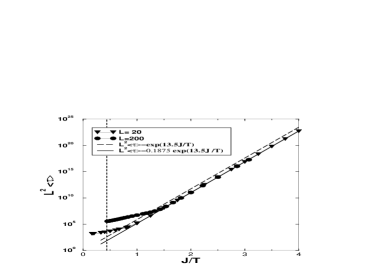
Figure 1: Mean lifetime, $\langle\tau\rangle$, in units of mcs as a function of $T^{-1}$ at $|H|$$=$$3J/4$ for the square lattice using the Glauber dynamic. The symbols are $s$$=$3 MCAMC data. The dashed line is the low-temperature prediction with the prefactor set to one, while the heavy solid line is with the correct prefactor of $3/16$ [16]. The vertical dashed line marks $T_{\rm c}$.

The MCAMC values obtained for the square-lattice lifetime at $|H|=3/4$ (so $\ell_{2}=3$) are shown in Fig. 1. Note that the average lifetime is very large. For $L=20$ if one Monte Carlo step per spin (MCSS) corresponded to about $10^{-13}$ sec then the largest time corresponds to about one year. The low temperature prediction with prefactor one (dashed line) does not describe the simulation data very well. However, including the low temperature prefactor [16] of $3/16$ for this field value (heavy solid line) fits the data very nicely.

Figure 2: Average lifetime, $T\ln(\langle\tau\rangle)$, in units of $J$ and $\langle\tau\rangle$ in units of mcs, as a function of $T$ for a $L=24$ square lattice using the Glauber dynamic. The symbols at finite $T$ are $s$$=$3 MCAMC data. The values of $|H|/J$ used, reading from the top, are $5/6$, 0.90, 0.95, 1.00, 1.05, and 1.10. The symbols at $T=0$ are the exact values of $\Gamma_{2}$, and the lines use the exact prefactor $A_{2}$. The prefactor is $3/8$ for $\ell_{2}=2$ ($J<|H|<2J$) and $3/16$ for $\ell_{2}=3$ ($2J/3<|H|<J$). The prefactor at $|H|=1$ is not known.

Figure 2 presents results for $T\ln\left(\langle\tau\rangle\right)$ which, with $\langle\tau\rangle$ in units of mcs, should equal $\Gamma_{2}+T\ln(A_{2})$. These are for $L=24$ for various $|H|$ values. The intercept is the exact low-temperature prediction, $\Gamma_{2}$, and the linear slope is the exact low-temperature prefactor, $A_{2}$. These data indicate that both the value of $\Gamma_{2}$ and the prefactor agree at low enough temperatures with the simulation data. However, exactly how low is low enough to agree with the data depends on the value of $|H|$. In particular, for values far from the special value where $\ell_{2}$ changes, the MCAMC values agree with the low-temperature predictions even for temperatures as large as $T=J/2$ (note $T_{c}\approx 2.26J$). However, closer to the special value where $\ell_{2}$ changes much lower temperatures are needed before agreement with the low-temperature predictions are seen. Hence the discontinuity in $\langle\tau\rangle$ due to the discontinuous prefactor is not seen in the simulation data.

5 Cubic-lattice Results

Figure 3 shows results for the sc lattice. The MCAMC and projective dynamics [19] results both agree with each other, and away from the values of $|H|$ where $\ell_{3}$ change they agree with the low-temperature prediction with the predicted prefactor [16]. At these special $|H|$ values $\Gamma_{3}$ decreases by $4J$. This would predict that near these values as $|H|$ decreases the lifetime of the metastable state would decrease. This is not physically intuitive, and the simulation data do show evidence of the predicted discontinuity for $T=0.2T_{\rm c}$.

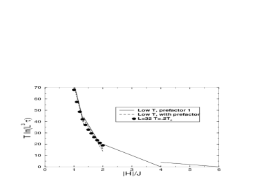
Figure 3: The average lifetime, $\langle\tau\rangle$, in units of Monte Carlo steps (mcs) as a function of $|H|$ at $T=0.2T_{\rm c}$ for the simple cubic lattice using the Glauber dynamic. The symbols are both MCAMC data using up to 3 transient states and projective dynamics simulations [19] . The heavy solid line is the low-temperature prediction with the prefactor set to one, while the dashed line segments are with the correct prefactor [16].

Figure 4 shows results of MCAMC simulations of the sc Ising model at low temperatures for various strong fields. No prefactors for these values (since $|H|>2J$) are predicted by [16]. For $4J<|H|<6J$ the prefactor can be evaluated using absorbing Markov chains, and is $7/6$. This result is consistent with the slope for $T<0.2J$.

The most striking result shown in Fig. 4 is that for both $|H|=3.5J$ and $|H|=3.9J$ the MCAMC results do not agree with the low-temperature predictions [16, 17, 18]. These are shown by the lowest corresponding symbols at $T=0$. An analysis of the path taken by the nucleating droplet shows that there is a higher saddle point than that predicted by the low-temperature results of Eq. 5. The value expected at this higher saddle point is shown by the higher corresponding symbols at $T=0$. For $3J\leq|H|\leq 4J$ this saddle has energy $28J-6|H|$, corresponding to an L-shaped droplet with three overturned spins. The region of $|H|$ for which there is a higher saddle point shrinks with increasing $\ell_{3}$, but is always finite near any non-zero value of $|H|$. This higher saddle point removes the discontinuity in $\Gamma_{3}$ near the values of $|H|$ where $\ell_{3}$ changes. In fact, $\Gamma_{3}$ is continuous for the corrected saddle, just as $\Gamma_{2}$ is continuous. The discontinuity in $\langle\tau\rangle$ due to a discontinous prefactor has not yet been supported by the MCAMC data for the sc lattice. One might expect the same behavior as seen in the square lattice, which keeps the discontinuity from being seen at any finite temperature.

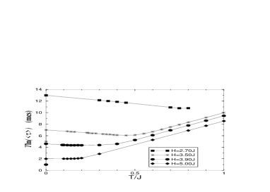
Figure 4: For the simple cubic lattice with Glauber dynamics, $T\ln\left(\langle\tau\rangle\right)$ is shown for several values of $|H|$. The symbols at finite $T$ are MCAMC data using up to $s=4$. For $|H|=2.7J$ below about $T=0.7J$ the MCAMC results seem to agree with a linear approach to the exact prediction, indicated by the same symbol at $T=0$. The same is also true for the results at $|H|=5J$ where the $T=0$ intercept is equal to 2. However, for both $|H|=3.5J$ and $|H|=3.9J$ the low-temperature predictions of Eq. 5 are not valid and do not fit the MCAMC results. These invalid results are shown by the lower corresponding symbols at $T=0$. Rather, the MCAMC results tend toward the corrected predictions given by the higher corresponding $T=0$ symbols.

6 Conclusions

The Monte Carlo with Absorbing Markov Chains (MCAMC) algorithm for long-time simulations of dynamics was described. The description was for the sc Ising ferromagnet, but can be generalized to other discrete systems. The $s=1$ MCAMC algorithm corresponds to the $n$-fold way algorithm [4] in discrete time [5]. In many cases the $s=1$ MCAMC can require many orders of magnitude less computer time than conventional dynamic simulations to perform the same calculation. The $s>1$ MCAMC can require many orders of magnitude less computer time than the $s=1$ MCAMC. These exponential decreases in computer time are accomplished without changing the underlying dynamic.

The MCAMC algorithm has been applied to check the low-temperature predictions for metastable decay in both the square and sc Ising ferromagnet. In particular, the predicted discontinuity in the average lifetime at the values of $|H|$ where the size of the droplet at the saddle point changes discontinuously was investigated. It was found that for the square lattice, where the discontinuity is only in the prefactor, a finite temperature simulation sees no evidence of this prefactor discontinuity. Instead, the temperature at which the simulations must be performed to see the low-temperature predictions decreases as the discontinuity is approached. For the sc lattice a discontinuity in both the prefactor and in the energy of the nucleating droplet was predicted [16, 17, 18]. No evidence for these discontinuities were found in the simulation data. The ‘exact formula’ for the cubic lattice nucleating droplet, Eq. 5, was rather found to be incorrect near the discontinuities. The corrected exact formula has no discontinuity in the energy of the nucleating droplet.
Acknowledgements
Special thanks to M. Kolesik for allowing inclusion of unpublished projective dynamic data. Partially funded by NSF DMR-9871455. Supercomputer time provided by the DOE through NERSC.

References

- [1] M.A. Novotny: Phys. Rev. Lett. 74, 1 (1995); erratum 75, 1424 (1995).
- [2] M.A. Novotny: in: Computer Simulation Studies in Condensed Matter Physics IX, ed. by D.P. Landau, K.K. Mon, H.-B. Shüttler (Springer-Verlag, Berlin, Heidelberg, 1997), p. 182.
- [3] M.A. Novotny: in Annual Reviews of Computational Physics IX, ed. by D. Stauffer (World Scientific, Singapore, 2001) p. 153.
- [4] A.B. Bortz, M.H. Kalos, J.L. Lebowitz: J. Comput. Phys. 17, 10 (1975).
- [5] M.A. Novotny: Comp. in Phys. 9, 46 (1995).
- [6] H.L. Richards, S.W. Sides, M.A. Novotny, P.A. Rikvold: J. Magn. Magn. Mater. 150, 37 (1995).
- [7] Ph.A. Martin: J. Stat. Phys. 16, 149 (1977).
- [8] K. Park, M.A. Novotny, this proceedings volume.
- [9] R.J. Glauber: J. Math. Phys. 4, 294 (1963).
- [10] G. Korniss, M.A. Novotny, P.A. Rikvold: J. Comput. Phys. 153, 488 (1999).
- [11] G. Korniss, Z. Toroczkai, M.A. Novotny, P.A. Rikvold: Phys. Rev. Lett. 84, 1351 (2000).
- [12] G. Korniss, M.A. Novotny, Z. Toroczkai, P.A. Rikvold: in Computer Simulation Studies in Condensed Matter Physics XIII, ed. by D.P. Landau, S.P. Lewis, H.-B. Schüttler (Springer Verlag, Heidelberg, 2001), p. 183.
- [13] J.D. Muñoz, M.A. Novotny, and S.J. Mitchell: in Computer Simulation Studies in Condensed Matter Physics XIII, ed. by D.P. Landau, S.P. Lewis, H.-B. Schüttler (Springer Verlag, Heidelberg, 2001), p. 92.
- [14] D.H. Bailey: ACM Trans. Math. Software 21, 379 (1995).
- [15] E. Jordão Neves, R.H. Schonmann: Commun. Math. Phys. 137, 209 (1991).
- [16] A. Bovier, F. Manzo: e-print cond-mat/0107376.
- [17] D. Chen, J. Feng, M. Qian: Science in China (Series A) 40, 832 (1997).
- [18] D. Chen, J. Feng, M. Qian: Science in China (Series A) 40, 1129 (1997).
- [19] M. Kolesik, M.A. Novotny, and P.A. Rikvold: Phys. Rev. Lett. 80, 3384 (1998).