Hartree-Fock dynamics in highly excited quantum dots

Abstract

Time-dependent Hartree-Fock theory is used to describe density oscillations of symmetry-unrestricted two-dimensional nanostructures. In the small amplitude limit the results reproduce those obtained within a perturbative approach such as the linearized time-dependent Hartree-Fock one. The nonlinear regime is explored by studying large amplitude oscillations in a non-parabolic potential, which are shown to introduce a strong coupling with internal degrees of freedom. This excitation of internal modes, mainly of monopole and quadrupole character, results in sizeable modifications of the dipole absorption.

Hartree-Fock (HF) theory is one of the most successful microscopic schemes to address finite Fermi systems, and usually the starting point of more refined approximations. Shortly after its proposal Dirac suggested a time-dependent extension (tdHF) that would account for dynamical processes [1] which has been the basis of many studies of oscillations in systems such as atoms, nuclei and molecules. Time-dependent HF theory is not restricted to small amplitude oscillations, although in this limit one obtains a scheme based on ground state perturbations which is not explicitly time dependent. In fact, one can obtain linearized equations (tdHF*) which are essentially equivalent to the well-known random-phase approximation (RPA) [2].

In this Letter we numerically study the tdHF evolution for electrons confined in a two-dimensional semiconductor quantum dot by direct integration of the time-dependent equations. We show the equivalence with the linearized tdHF* approach previously used by one of us [3] and, at the same time, prove the minor role of the ground state symmetry-breaking on the far-infrared (FIR) absorption. We also explore the nonlinear regime by going to the large amplitude limit where we find a fast energy transfer from dipole to internal breathing and quadrupole oscillations, made possible by the non-parabolicity of the confining potential. The excitation of internal breathing and quadrupole modes results in sizeable modifications of the dipole absorption, as compared to the small amplitude case.

As described in many textbooks, the essential ingredient of tdHF theory is the description of the state of the system at any time of the dynamic evolution by a single Slater determinant, built with single-particle orbitals. Given initial conditions, the central equations of the theory provide the time evolution of the orbital set $\{\varphi_{i\eta}({\bf r},t)\}$. The orbital labels indicate state number ($i$) and spin $z$-projection ($\eta=\uparrow,\downarrow$). The tdHF equations for electrons confined to the $xy$ plane by an external $v_{ext}({\bf r},t)$ and vector ${\bf A}({\bf r})=B/2(-y,x)$ potentials read [4]

$$i\frac{\partial}{\partial t}\varphi_{i\eta}({\bf r}_{1},t) = \left[\rule{0.0pt}{17.07182pt}\frac{1}{2}\left(-i\nabla+\gamma{\bf A}({\bf r}_{1})\right)^{2}+v_{H}({\bf r}_{1},t)\right.$$ (1)

$$+ \left.v_{ext}({\bf r}_{1},t)\,+\frac{1}{2}g^{*}m^{*}\gamma Bs_{z}\rule{0.0pt}{17.07182pt}\right]\varphi_{i\eta}({\bf r}_{1},t)$$ (2)

$$- \int{d{\bf r}_{2}\,\frac{\rho_{\eta}({\bf r}_{1},{\bf r}_{2},t)}{r_{12}}\,\varphi_{i\eta}({\bf r}_{2},t)}\;,$$ (3)

where we have defined $\gamma=e/c$ and the Hartree potential $v_{H}({\bf r}_{1},t)=\int{d{\bf r}_{2}\,\rho({\bf r}_{2},t)/r_{12}}$, given in terms of the total density $\rho({\bf r},t)$. In Eq. (1) we have also defined the one-body density-matrix entering the exchange integral

$$\rho_{\eta}({\bf r}_{1},{\bf r}_{2},t)=\sum_{j,occ.}{\varphi_{j\eta}({\bf r}_{1},t)\,\varphi^{*}_{j\eta}({\bf r}_{2},t)}\;.$$ (4)

In this work we shall present direct numerical solutions of Eq. (1) obtained by discretizing the equations both in space, into a uniform grid of points, and in time $t_{k}=k\Delta t$ by using the Cranck-Nicholson algorithm [5]. Specifically, by calling $h_{0}^{(k)}$ and ${\cal V}_{i\eta}^{(k)}$ the local term (within square brackets) and the exchange integral in Eq. (1) at time-step $k$, the algorithm reads

$$\left(1+{i\Delta t\over 2}h_{0}^{(k+1)}\right)\varphi_{i\eta}^{(k+1)} = \left(1-{i\Delta t\over 2}h_{0}^{(k)}\right)\varphi_{i\eta}^{(k)}$$ (5)

$$+ {i\Delta t\over 2}\left({\cal V}_{i\eta}^{(k)}+{\cal V}_{i\eta}^{(k+1)}\right)\;.$$ (6)

As a first guess, we assume $h_{0}^{(k+1)}=h_{0}^{(k)}$ and ${\cal V}_{i\eta}^{(k+1)}={\cal V}_{i\eta}^{(k)}$ which allows an initial solution of (5). Subsequently $h_{0}^{(k+1)}$ and ${\cal V}_{i\eta}^{(k+1)}$ are updated and the process repeated untill convergence in $\varphi_{i\eta}^{(k+1)}$ is found (typically 4-8 iterations are enough for a sufficiently small $\Delta t$).

The system strength function $S(\omega)$, or equivalently the absorption cross section $\sigma(\omega)=\omega S(\omega)$ are easily determined from the time signals $\langle\sum_{i}{{\bf r}_{i}}\rangle(t)$ by means of a frequency analysis, in a much similar way as used in real-time Density-Functional calculations of atomic clusters [6, 7] and quantum dots [8]. Important differences with the latter are the exact treatment of the exchange (neglecting correlation though) and the possibility to explore large amplitude oscillations since the formalism is not centered on a ground-state energy functional.

In the limit of small oscillation amplitudes we compare with a frequently used linearized version (tdHF*), which provides the linear response to an external oscillating dipole potential adiabatically switched on

$${\phi}^{\mathrm{e}xt}({\bf r},t)={\cal E}^{\mathrm{e}xt}r\exp\left[\pm i\theta-i(\omega+i\eta)t\right]\;,$$ (7)

with $(r,\theta)$ the polar coordinates, $\eta\rightarrow 0^{+}$ and $`\pm^{\prime}$ labelling the two circular polarization states. The power absorbed by the system is

$$P(\omega) = 2\pi\,\omega{\cal E}^{\mathrm{e}xt}\sum_{\alpha\beta}\langle\beta|r|\alpha\rangle\delta_{M_{\beta},{M_{\alpha}\pm 1}}\times$$ (9)

$$\Im\left\{f^{\alpha\beta}(\omega)\langle\alpha|\phi^{\mathrm{s}c}|\beta\rangle\right\},$$

where $\phi^{\mathrm{s}c}$ is the self-consistent electrostatic potential found from the external perturbation $\phi^{\mathrm{e}xt}$ via the dielectric tensor [3], and

$$f^{\alpha\beta}(\omega)=\frac{f^{0}_{\beta}-f^{0}_{\alpha}}{\omega+(\omega_{\beta}-\omega_{\alpha})+i\eta}\;,$$ (10)

with $f^{0}$ the equilibrium Fermi distribution. Notice that within the tdHF* we require the angular part of the orbitals to be simple phases $e^{iM\theta}$, which amounts to assuming circular symmetry of the density and mean field.

Most of the system physical properties are determined by the external potential $v_{ext}(r)$, which we shall assume to be static and circularly symmetric. Following Ref. [9] we consider a step in the radial direction separating two regions with a different slope in the potential. This type of behaviour reproduces to some extent the effective potential in quantum dot arrays, where lattice periodicity introduces a deviation from a pure quadratic radial law. The specific parametrization we use is

$$v_{ext}(r) = v_{1}(r)\,f_{1}(r)+\left[v_{2}(r)\right.$$ (11)

$$+ \left.v_{1}(R_{0})-v_{2}(R_{0})+\Delta\right]\,f_{2}(r)\;,$$ (12)

where $R_{0}$ and $\Delta$ are the step position and height, respectively. In Eq. (11) $v_{1,2}(r)$ indicate the potential in the $r<R_{0}$ ($r>R_{0}$) region and $f_{1,2}(r)$ is a smooth switching function. Namely, these region-dependent functions are

$$v_{1,2}(r) = \frac{1}{2}\omega_{1,2}\,r^{2}$$ (13)

$$f_{1,2}(r) = \frac{1}{2}\left(1\mp\tanh{r-R_{0}\over\sigma}\right)\;.$$ (14)

In the calculations shown below we consider a system with $N=6$ electrons and $R_{0}=30$ nm, $\sigma=5$ nm, $\omega_{1,2}=3.37$ meV, $\Delta=6$ meV. This particular set of values is motivated by the experiments in Ref. [9].

Figure 1 displays the dipole absorption in the small amplitude regime obtained within tdHF and tdHF*. As is well known from Kohn’s theorem, in purely parabolic dots the FIR absorption consists of two bands at energies

$$\omega_{\pm}=\sqrt{\omega_{0}^{2}+(\omega_{c}/2)^{2}}\pm\omega_{c}/2\;$$ (15)

where $\omega_{c}=eB/c$ is the cyclotron frequency. Looking at the lower panel of Fig 1, one can indeed identify a low energy peak around 2 meV and a higher-energy structure with two peaks. The existence of a structured high energy band is in agreement with the experiments [9] and as seen in Fig. 1 the two methods yield very similar results, showing the equivalence of the very different techniques in this limit. Quite remarkably, at $B=1$T HF provides a symmetry broken ground state, with the six electrons localized in a ring-like structure similar to those discussed by Yannouleas and Landman [10] or Manninen et al. [11], which is obviously not present within the circular HF*. Nevertheless, Fig. 1 shows that the absorption obtained from the symmetry-broken ground state does not importantly differ from that of the circular solution, proving that the details of the FIR absorption are not much sensitive to the internal structure. For a purely parabolic dot there is a complete independence of the FIR absorption and the internal symmetry but it is a remarkable fact that for the more realistic dot potential (11) the details of the high energy branch are not sensitive to the internal structure.

We turn next to large amplitude oscillations within tdHF. Figure 2 shows the center of mass trajectory following an initial rigid displacement to the point indicated in the upper right corner. This is a dramatic perturbation which amounts to an excitation energy of $\Delta E=26.5$ meV, to be compared with a ground state energy of $E=112.7$ meV. A relevant observation in Fig. 2 is that the amplitude of the oscillation dampens in time, hinting at an important energy transfer from the center of mass to the internal degrees of freedom which are evolving in time. To better monitor this coupling mechanism we introduce the internal coordinates $\tilde{\bf r}={\bf r}-{\bf R}_{cm}$, where ${\bf R}_{cm}$ is the center of mass position, and define the internal quadrupole and monopole operators as

$$\tilde{Q} = \sum_{i}{\tilde{x_{i}}\tilde{y_{i}}}=\sum_{i}{x_{i}y_{i}}-\frac{1}{N}\sum_{ik}{x_{i}y_{k}}$$ (16)

$$\tilde{M} = \sum_{i}{\tilde{x_{i}}^{2}+\tilde{y_{i}}^{2}}=\sum_{i}{x_{i}^{2}+y_{i}^{2}}-\frac{1}{N}\sum_{ik}{x_{i}x_{k}+y_{i}y_{k}}\;.$$ (17)

Notice that these internal probes involve two-body operators when expressed in the fixed laboratory frame.

Figure 3 shows the time signals corresponding to the large amplitude displacement of Fig. 2 as well as the results following a much smaller perturbation corresponding to the linear regime. As expected from the previous figure, the large oscillation dipole signal is reducing its amplitude in time, while the internal quadrupole and monopole modes get highly excited. The breathing-mode result is actually indicating that the dot expands after a rather short time, and keeps oscillating around the expanded configuration. This energy transfer to the breathing mode is not seen in the small amplitude regime, where only minor oscillations around the ground state configuration are always found. As already mentioned, the mechanism observed here is possible due to the non-parabolic confining potential permitting the energy transfer between modes, showing that nonlinear processes associated with high energy excitations can effectively induce strong internal excitations.

The frequency analysis of the large amplitude signal is complicated by the decrease in amplitude. An approximate treatment is still possible by defining a time window in which the variations are not too large. In fact the frequency spectrum evolves smoothly in time, depending on the window position. For large times the result is not much sensitive on this position and is shown in Fig. 4 for $B=1$T. Notice that in the frequency analysis of the time signal each peak is represented by a Lorentzian having an artificially chosen width $\Gamma$, for an easier representation of the spectrum. Although experimentally rather large $\Gamma$’s are usually found, in Fig. 4 we show the result obtained using either a large or a small value of $\Gamma$, in order to clearly display the fine structure of the absorption.

An important fragmentation appears in the large amplitude spectrum of Fig. 4, due the splitting in many closely lying peaks. Actually, the three upper sharp transitions of the small amplitude spectrum transform into a bunch of peaks. Within a one-particle picture, we attribute this effect to the large fluctuation of the mean field, seen from the internal signals, which causes also important variations in the effective single particle energies and in the corresponding particle-hole transitions. Interestingly enough, when using a large (and more realistic) $\Gamma$ we obtain a narrowing of the high energy branch, roughly covering the interval $[4.75,5.5]$ eV. In the small amplitude case the higher branch, composed of three peaks, approximately lies at $[4.25,5.5]$ eV. The observed effect is thus a dynamical narrowing of the high energy branch induced by the large amplitude oscillation.

To summarize, the tdHF equations have been integrated in time to describe electronic oscillations in two-dimensional quantum dots confined by a circular non-parabolic potential. In the limit of small amplitudes the results are very similar to those obtained in the linearized version of the circularly constrained theory (tdHF*). The symmetry broken ground states do not significantly modify the dipole absorption in this regime. The nonlinear behaviour has been investigated by using large amplitude initial displacements. An effective transfer from the center of mass dipole to internal monopole and quadrupole modes has been observed in this case, thus providing a mechanism to strongly excite internal modes in non-parabolic dots. Additionally, the large amplitude motion has been found to induce a dynamical narrowing of the dipole absorption. This effect would manifest in absorption experiments using a high-intensity far-infrared radiation.

This work was supported in part by Grant No. PB98-0124 from DGESeiC, Spain, the Research Fund of the University of Iceland, and the Icelandic Natural Science Council.

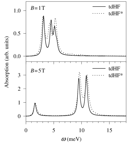
FIG. 1.: The power absorption for 6 electrons obtained within tdHF and using the linear version with circular symmetric tdHF*, for two different values of the magnetic field $B$.

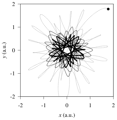
FIG. 2.: Center of mass trajectory following a large initial displacement to the point in the upper rigth corner, obtained within tdHF for the quantum dot considered in this work at $B=1$T. Dotted, thin solid and thick solid lines indicate the motion in subsequent intervals of $\approx 12$ ps, respectively. See text.

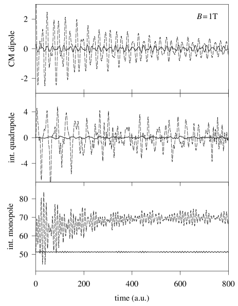
FIG. 3.: Time dependence of the center of mass (CM) dipole, internal quadrupole and internal monopole signals in the small (solid) and large (dashed) amplitude regimes at $B=1$ T.

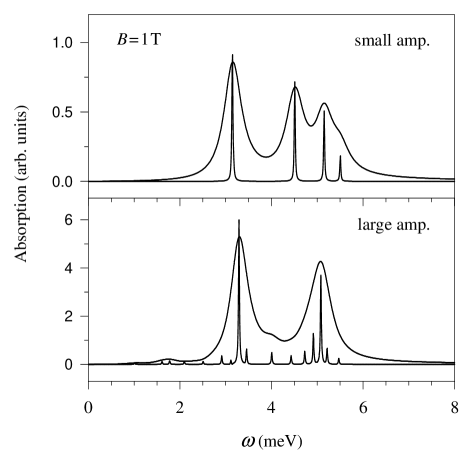
FIG. 4.: Dipole absorption corresponding to the small (upper panel) and large (lower panel) amplitude signals of Fig. 3. Two different peak widths have been used for a better presentation. The large amplitude results are obtained from the time window [500,800] a.u.

REFERENCES

- [1] P. A. M. Dirac, Proc. Cambridge Philos. Soc. 26, 376 (1930).
- [2] J.P. Blaizot and G. Ripka, Quantum theory of finite systems (MIT press, Cambridge, 1986).
- [3] V. Gudmundsson and A. S. Loftsdóttir, Phys. Rev. B 50, 17433 (1994).
- [4] Unless stated otherwise, we shall use effective atomic units (for which , with and the dielectric constant and electron effective mas, respectively) corresponding to GaAs values, i.e., and with . Therefore the energy, length and time effective units are H meV, Å and fs, respectively. The effective gyromagnetic factor is for bulk GaAs.
- [5] W. H. Press, B. P. Flannery, S. A. Teukolsky, and W. T. Vetterling, Numerical Recipes (Cam. Univ. Press, Cambridge, 1986).
- [6] K. Yabana and G. F. Bertsch, Phys. Rev. B 54, 4484 (1996).
- [7] F. Calvayrac, P.-G. Reinhard, E. Suraud, Ann. Phys. (NY) 255, 125 (1997).
- [8] A. Puente, Ll. Serra, Phys. Rev. Lett. 83, 3266 (1999).
- [9] R. Krahne, V. Gudmundsson, C. Heyn, and D. Heitmann, Phys. Rev. B 63, 195303 (2001).
- [10] C. Yannouleas and U. Landman, Phys. Rev. Lett. 82, 5325 (1999).
- [11] M. Koskinen, M. Manninen, B. Mottelson, and S. M. Reimann, Phys. Rev. B 63, 205323 (2001).