Neural Representation of Probabilistic Information

Abstract

It has been proposed that populations of neurons process information in terms of probability density functions (PDFs) of analog variables. Such analog variables range, for example, from target luminance and depth on the sensory interface to eye position and joint angles on the motor output side. The requirement that analog variables must be processed leads inevitably to a probabilistic description, while the limited precision and lifetime of the neuronal processing units leads naturally to a population representation of information. We show how a time-dependent probability density $\rho(x;t)$ over variable $x$, residing in a specified function space of dimension $D$, may be decoded from the neuronal activities in a population as a linear combination of certain decoding functions $\phi_{i}(x)$, with coefficients given by the $N$ firing rates $a_{i}(t)$ (generally with $D<<N$). We show how the neuronal encoding process may be described by projecting a set of complementary encoding functions ${\hat{\phi}}_{i}(x)$ on the probability density $\rho(x;t)$, and passing the result through a rectifying nonlinear activation function. We show how both encoders $\hat{\phi}_{i}(x)$ and decoders $\phi_{i}(x)$ may be determined by minimizing cost functions that quantify the inaccuracy of the representation. Expressing a given computation in terms of manipulation and transformation of probabilities, we show how this representation leads to a neural circuit that can carry out the required computation within a consistent Bayesian framework, with the synaptic weights being explicitly generated in terms of encoders, decoders, conditional probabilities, and priors.

1 Introduction

It has been hypothesized (Anderson, 1994, 1996) that circuits of cortical neurons perform statistical inference, and, in particular, that they encode and process information about analog variables in the form of probability density functions (PDFs). This PDF hypothesis provides a unified framework for understanding diverse observations from experimental neurobiology, constructing neural network models, and gaining insights into how neurons can implement a rich collection of information-processing functions.

The PDF hypothesis derives from two major themes of computational neuroscience. The first theme stems from efforts to determine how information is represented by neural systems, through understanding how neural activity correlates to external cues or actions (such as sensory stimuli or motor response). Our understanding of neural encoding can be tested by inferring sensory input or motor output from a set of neural activities, and comparing the estimate thus obtained to the external cue or action.

To decode the response from a population of neurons requires procedures to infer information from individual spike trains, as well as procedures to combine these results into an aggregate estimate. An optimal method for decoding information from individual neural spike trains has been developed [Bialek et al., 1991, Bialek and Rieke, 1992, Rieke et al., 1997] and applied to movement-sensitive neurons in the blowfly [Rieke et al., 1997] and to other systems [Theunissen et al., 1996]. This method consists of utilizing a linear filter to extract the maximum possible information from each spike (typically a few bits; see Rieke et al., 1997), as measured by the ability to reconstruct the stimulus from the spike train. In these studies, the linear filter determines a firing rate from the spike trains; this firing rate contains most of the information, with additional information possibly encoded in other aspects of the activity patterns. In the current work, we assume that the firing rates capture the essential behavior of neural systems, and will not explicitly consider spike trains.

Methods for decoding information from the firing rates of populations of neurons were pioneered by Georgopoulos and collaborators. They showed that a “population vector” derived from the firing rates of a population of cortical neurons can be used to predict the intended arm movements of monkeys [Georgopoulos et al., 1986, Schwartz, 1993]. This vector estimate of direction, $\mathbf{V}_{\mathrm{est}}$, is obtained from the neural firing rates $a_{i}$ by

$$\mathbf{V}_{\mathrm{est}}=\sum_{i=1}^{N}a_{i}\mathbf{C}_{i}$$ (1)

where the preferred direction vectors, $\mathbf{C}_{i}$, indicate the direction at which neuron $i$ has its maximal firing response. The population vector approach has been refined and extended by several authors; in particular, Salinas and Abbott (1994) provide an excellent discussion of several such refinements, as well as introducing their own. The emphasis in such studies has been the reconstruction of vector quantities from populations of neural responses by a process that in several cases appears to be computation of an expectation value from an implicit probability distribution.

The second theme leading to the PDF hypothesis stems from an analysis showing that the original Hopfield neural network implements, in effect, Bayesian inference on analog quantities in terms of PDFs [Anderson and Abrahams, 1987]. The role of PDFs in neural information processing is being explored along a number of avenues. As in the present work, Zemel et al. (1998) have investigated population coding of probability distributions, but with different representations than those we will consider here. Several extensions of this representation scheme have been developed [Zemel, 1999, Zemel and Dayan, 1999, Yang and Zemel, 2000] that feature information propagation between interacting neural populations. Further, a number of related models have been introduced. Of particular note is a dynamic routing model of directed attention (Anderson and Van Essen, 1987; Olshausen et al., 1993, 1995). Additionally, several “stochastic machines” [Haykin, 1999] have been formulated, including Boltzmann machines [Hinton and Sejnowski, 1986], sigmoid belief networks [Neal, 1992], and Helmholtz machines [Dayan and Hinton, 1996]. Stochastic machines are built of stochastic neurons that choose one of two possible states in a probabilistic manner. Learning rules for stochastic machines enable such systems to model the underlying probability distribution of a given data set; however, they are not biologically realistic.

The two prominent themes of population coding and probabilistic inference are combined in the PDF hypothesis through the assertion that a physical variable $x$ is described by a neural population at time $t$ in terms of a PDF $\rho(x;t)$, rather than as a single-valued estimate $x(t)$. Such a PDF description has the significant advantage that it not only permits a single-valued estimate to be calculated, but also provides for measures of the uncertainty of such estimates. For example, a specific value $\xi$ at time $t$ can be represented as the mean of a normal distribution over $x$ with variance $\sigma^{2}$, so that

$$\rho(x;t)=N\left(x;\xi(t),\sigma^{2}(t)\right)$$ (2)

Clearly, this PDF allows $\xi(t)$ to be known very precisely (small variance) or with a great deal of uncertainty (large variance).

More generally, we consider a PDF described at time $t$ in terms of a set of $D$ underlying parameters $\left\{A_{\mu}\right\}$. Guided by the experimentally observed linear decoding rules discussed above, we will take the PDFs to be represented by

$$\rho(x;t)\equiv\rho\left(x;\left\{A_{\mu}(t)\right\}\right)=\sum_{\mu=1}^{D}A_{\mu}(t)\Phi_{\mu}(x)$$ (3)

The basis functions $\Phi_{\mu}(x)$ are orthonormal functions that define the PDFs the neural circuit can represent. We describe $x$ with $\rho(x;\left\{A_{\mu}(t)\right\})$ rather than $\rho(x\!\mid\!\left\{A_{\mu}(t)\right\})$ to distinguish between the assumed forms of models (equation 3) and relationships that exist amongst random variables (viz. conditional probabilities).

The amplitudes $A_{\mu}(t)$ of the representations defined by equation 3 cannot be interpreted as neuronal firing rates: they can take on negative values and are more precise than neuronal firing rates. However, we can represent a PDF in terms of decoding functions $\phi_{i}(x)$ and firing rates $a_{i}(t)$ associated with $N$ neurons, so that

$$\rho(x;t)=\sum_{i=1}^{N}a_{i}(t)\phi_{i}(x)$$ (4)

Unlike the basis functions $\Phi_{\mu}(x)$, the decoding functions $\phi_{i}(x)$ form a highly redundant, overcomplete representation ($N\gg D$) that is specialized for use with neurons of limited precision.

From the relations asserted in equations 3 and 4, we can identify three relevant problem domains. First, we have the physical variable $x$, described by the PDF $\rho(x;t)$. This domain is that of high-level concepts. Second, we have the neural network with its measurable neural firing rates $a_{i}(t)$. The neural network constitutes a physical implementation of the desired computations on the physical variable, so the properties of this second domain should be chosen to match the properties of biological systems as closely as possible. In particular, the neural firing rates must be constrained to be positive quantities of low precision. The third domain is that of the underlying parameters $A_{\mu}$, which subserve an alternative, abstract implementation of the desired computations. The constraint in this case is minimality: we concern ourselves only with mathematical convenience and allow the $A_{\mu}$ to be of arbitrary precision and to take on negative values.

Following Zemel et al. (1998), the domain of physical variables is called the implicit space and the domain of measurable quantities the explicit space. Extending their nomenclature, we shall refer to the third domain as the minimal space. The minimal space will serve as a useful bridge between the two other spaces.

It may be conceptually helpful to regard the variables or parameters $A_{\mu}(t)$ as the activities of a set of $D$ “metaneurons,” fictitious entities that reside and act in the minimal space. However, it must be emphasized that such metaneurons differ from real neurons in their abilities to function with high precision and to produce negative “firing rates” $A_{\mu}(t)$. Accordingly, they possess valuable properties that will facilitate formal representation and analysis.

2 Obtaining the Neuronal Representation

2.1 Multiple Levels of Representation

The fundamental assumption of the framework to be developed in this paper is that information about a physical variable $x$ given a set of parameters $\mathbf{A}=\left\{A_{1},A_{2},A_{3},\ldots\right\}$ at time $t$ is represented by an ensemble of neurons as a PDF $\rho(x;A_{1}(t),A_{2}(t),A_{3}(t),\ldots)$. For notational convenience, we will usually abbreviate this quantity as $\rho(x;t)$. This PDF can be determined from a set of neuronal firing rates $\{a_{i}(t)\}$ using a set of decoding functions (or simply decoders) $\phi_{i}(x)$, as prescribed in equation 4. In turn, a set of encoding functions (encoders) $\hat{\phi}_{i}(x)$ is used to determine the firing rates from an assumed PDF by means of

$$a_{i}(t)=f\left(\int\hat{\phi}_{i}(x)\rho(x;t)dx\right)$$ (5)

where a nonlinear activation function $f()$ is introduced to preclude negative firing rates. The encoding functions $\hat{\phi}_{i}(x)$ must be chosen so as to yield a close match to desired (i.e. experimentally observed) firing rates $a_{i}(t)$. The decoding rule (equation 4) should in general be viewed as only returning an approximation to the PDF: in particular, functions that are not strictly positive semidefinite can be decoded from such a rule.

We can also represent the PDF using a complete orthonormal basis $\left\{\Phi_{\mu}(x)\right\}$ for the space spanned by the decoders, as shown in equation 3. Further, we can represent the decoding functions in terms of this basis, writing

$$\phi_{i}(x)=\sum_{\nu=1}^{D}\kappa_{\nu i}\Phi_{\nu}(x)$$ (6)

where the $\kappa_{\nu i}$ are coupling coefficients to be determined. Since we now have an orthonormal basis, the coefficients $A_{\mu}$ in equation 3 are simply evaluated from

$$A_{\mu}(t)=\int\Phi_{\mu}(x)\rho(x;t)dx$$ (7)

The encoding and decoding rules based on the amplitudes $A_{\mu}(t)$ in the minimal space are seen to parallel those based on the neuronal firing rates $a_{i}(t)$, apart from the absence of a nonlinearity in equation 7. In this section, we will develop methods to relate operations in the mathematically convenient minimal space and the biologically plausible implementation of PDFs in the explicit space of model neurons.

2.2 Obtaining the Encoding Functions

Although we do not know the encoding functions at this point, we do know that they can be represented in terms of another set of basis functions $\left\{\hat{\Phi}_{\mu}(x)\right\}$ through

$$\hat{\phi}_{j}(x)=\sum_{\mu}\hat{\kappa}_{j\mu}\hat{\Phi}_{\mu}(x)$$ (8)

where the coupling coefficients $\hat{\kappa}_{j\mu}$ are in general distinct from the $\kappa_{\nu i}$. For many networks, it is appropriate to assume the basis for the encoders to be identical to the basis for the decoders. For example, in the case of the neural integrator (see section 2.5) the PDFs are continually mapped into and out of the minimal space provided by the $\Phi_{\mu}(x)$ and $\hat{\Phi}_{\nu}(x)$. Thus, $\mathrm{span}\left\{\Phi_{\mu}\right\}$ can be equal to $\mathrm{span}\left\{\hat{\Phi}_{\nu}\right\}$. For definiteness, we take $\Phi_{\mu}(x)=\hat{\Phi}_{\mu}(x)$.

To find the encoding functions, we define the cost function

$$E_{1} = {1\over 2}\sum_{i}\int\left[a_{i}(\mathbf{A})-f\left(\int\hat{\phi}_{i}(x)\rho(x;\mathbf{A})dx\right)\right]^{2}\rho(\mathbf{A})d\mathbf{A}$$

$$= {1\over 2}\sum_{i}\int\left[a_{i}(\mathbf{A})-f\left(\sum_{\nu}\hat{\kappa}_{i\nu}\int\Phi_{\nu}(x)\rho(x;\mathbf{A})dx\right)\right]^{2}\rho(\mathbf{A})d\mathbf{A}$$

We now use gradient descent to determine the $\hat{\kappa}_{i\nu}$ that minimize $E_{1}$

$${d\hat{\kappa}_{j\mu}\over dt}\approx-\eta{\partial E_{1}\over\partial\hat{\kappa}_{j\mu}}=\int\left(a_{j}(\mathbf{A})-f(h_{j}(\mathbf{A}))\right)f^{\prime}(h_{j}(\mathbf{A}))U_{\mu}(\mathbf{A})\rho(\mathbf{A})d\mathbf{A}$$ (10)

where $\eta$ is a rate constant. We have defined

$$U_{\nu}(\mathbf{A})=\int\Phi_{\nu}(x)\rho(x;\mathbf{A})dx$$ (11)

$$h_{j}(\mathbf{A})=\sum_{\nu}\hat{\kappa}_{j\nu}U_{\nu}(\mathbf{A})$$ (12)

to simplify the expression.

To verify the efficacy of this optimization procedure, we apply it to a set of broadly tuned, biologically reasonable neuronal responses to a precise input signal. In particular, we use piecewise-linear activities (Figure 1), essentially one-dimensional versions

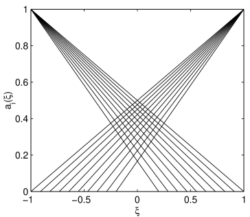
Figure 1: Broad piecewise-linear functions provide biologically plausible neural firing rates. These firing profiles are similar to one-dimensional versions of the neural responses used to construct Georgopoulos’s population vector.

of the response functions entering Georgopoulos’s population vector, to define our neural responses over the interval $[-1,1]$ (see also Figure 4 in Fuchs et al., 1988). We assume a minimal space spanned by two straight-line functions, shown in Figure 2a,

a

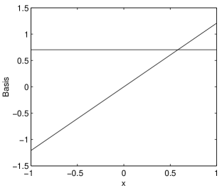
b

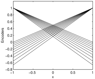
c

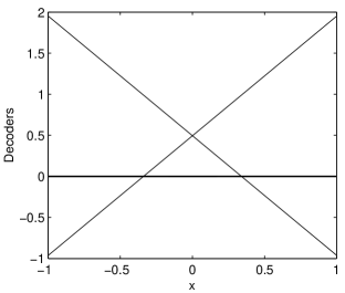
d

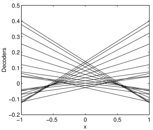
Figure 2: Encoders and decoders obtained using the optimization procedures of sections 2.2 and 2.3. (a) An orthonormal basis for the minimal space underlying the piecewise-planar firing rates. Any line segment over the interval $[-1,1]$ can be expressed as a linear combination of these two basis functions. (b) Encoders found using the optimization procedure. For each neuron, the encoder has a slope identical to that of the firing-rate profile. (c) Decoders obtained in the absence of noise require neurons of extreme precision to operate properly. Two decoders significantly contribute to the decoded PDFs, while all others are zero, contributing nothing to the decoded PDF. (d) Decoders obtained assuming a small amount of noise depend upon all of the neurons. The decoders shown here result from a noise variance of 0.01, limiting the precision of the neurons to biologically plausible levels. Note that these decoders can take on negative values, so the functions reconstructed from the neural firing rates may only approximate the encoded PDF.

and take the activation function to be rectification

$$f(x)=\left\{\begin{array}[]{cc}x&x\geq 0\\ 0&x<0\end{array}\right.$$ (13)

Since we are interested in representing a precise input, we choose $\rho(x;t)=\delta(x-\xi(t))$. Applying the optimization procedure, we obtain a set of encoders (Figure 2b) that are able to exactly reconstruct the neural activity patterns with input PDFs of the assumed Dirac delta function form.

2.3 Obtaining the Decoding Functions

A similar procedure is used to find the decoding functions. We first account for the limited precision of neural firing rates and for any intrinsic noise of real neurons by converting the neural firing rates into stochastic processes

$$a_{i}(\mathbf{A})\rightarrow a_{i}(\mathbf{A})+\varepsilon_{i}$$ (14)

where $\varepsilon_{i}$ represents the noise source. We assume $\varepsilon_{i}$ to have zero mean without loss of generality; a non-zero mean can be absorbed into the firing rate profiles, if needed. The above encoding functions are unchanged by the presence of zero-mean noise.

To ensure that the encoders and decoders found are not dependent on a particular realization of the noise, we define the cost function

$$E_{2}={1\over 2}\left\langle\int\!\!\!\int\left(\rho(x;\mathbf{A})-\sum_{i=1}^{N}\left(a_{i}(\mathbf{A})+\varepsilon_{i}\right)\phi_{i}(x)\right)^{2}\rho(\mathbf{A})dxd\mathbf{A}\right\rangle_{\left\{\varepsilon_{i}\right\}}$$ (15)

Here, the angle brackets indicate an ensemble average over realizations of the neuronal noise. Substituting equation 6 into $E_{2}$, we have

$$E_{2}={1\over 2}\left\langle\int\!\!\!\int\left(\rho(x;\mathbf{A})-\sum_{i,\nu}\Phi_{\nu}(x)\kappa_{\nu i}\left(\vphantom{A_{i}^{i}}a_{i}(\mathbf{A})+\varepsilon_{i}\right)\right)^{2}\rho(\mathbf{A})dxd\mathbf{A}\right\rangle_{\left\{\varepsilon_{i}\right\}}$$ (16)

To find the $\kappa_{\nu i}$ that minimize this cost function, we calculate ${\partial E_{2}}/{\partial\kappa_{\nu j}}$. Taking each $\varepsilon_{i}$ to be independent, identically distributed, zero-mean Gaussian noise with variance $\sigma^{2}$ produces

$$\frac{\partial E_{2}}{\partial\kappa_{\nu j}}=-M_{\nu j}+\sum_{i}\kappa_{\nu i}\left(\Gamma_{ij}+\sigma^{2}\right)$$ (17)

where

$$M_{\nu j}=\int\!\!\!\int\rho(x;\mathbf{A})a_{j}(\mathbf{A})\Phi_{\nu}(x)\rho(\mathbf{A})dxd\mathbf{A}$$ (18)

and

$$\Gamma_{ij}=\int a_{i}(\mathbf{A})a_{j}(\mathbf{A})\rho(\mathbf{A})d\mathbf{A}$$ (19)

Setting the derivatives to zero and recasting equation 19 in matrix form, we have

$$\left(\Gamma+\sigma^{2}I\right)\kappa=M$$ (20)

We can solve directly for $\kappa$ by inverting $\left(\Gamma+\sigma^{2}I\right)$.

The inclusion of noise is essential for producing sensible decoders. To illustrate this fact, we determine decoders for neurons with piecewise-linear activity patterns employing the basis shown in Figure 2a (discussed in section 2.2). The decoders are used to attempt a reconstruction of the original delta-function PDFs, inverting the encoding process previously considered. With $\sigma^{2}=0$, the algorithm produces two decoders that play a significant role while the others are all zero (Figure 2c). This noise-free solution evidently requires neurons that are extremely precise in their firing rates, rather than making use of redundant neurons to improve the quality of the representation. With noise present ($\sigma^{2}>0$), we determine a set of decoders that utilizes all of the neurons in the representation (Figure 2d) and is independent of unrealistically precise firing rates.

Having determined the decoders, we can directly transform between the explicit, implicit, and minimal spaces. The transformation rules are summarized pictorially in Figure 3.

Figure 3: Transformations between the representations. With the indicated rules, we can readily switch between the implicit, explicit, and minimal spaces, associated respectively with the variables $x$, $a_{i}$ ($i=1,2,3,\ldots,N$), and $A_{\mu}$ ($\mu=1,2,3,\ldots,D$), and select the most convenient one for any given task.

2.4 Dimensionality of the Minimal Space

The structure of the neural representations created depends critically upon the dimensionality $D$ of the associated spaces. We can most easily explore the effect of the dimensionality in the minimal space, where $D$ is simply equal to the number of basis functions $\Phi_{\mu}(x)$.

By way of illustration, let us pattern the basis functions after the Legendre polynomials $P_{\mu}(x)$. The Legendre polynomials form an orthogonal set, but are not normalized, so we define $\tilde{P}_{\mu}(x)={P_{\mu}(x)}/\sqrt{{\int_{-1}^{1}P_{\mu}^{2}(x)dx}}$ over the interval $[-1,1]$. For dimension $D$, we then set the minimal-space basis function $\Phi_{\mu}(x)$ equal to the normalized Legendre polynomial $\tilde{P}_{\mu-1}(x)$ for $\mu=1,2,\ldots D$.

To demonstrate the effect of the dimension $D$ upon the quality of the neural representation, we compare an assumed target PDF with the PDF as represented in neural populations. We vary $D$ and generate, as described in sections 2.2 and 2.3, encoding and decoding functions optimized to work with neurons with firing rate profiles as shown in Figure 1. Using equation 5, the target PDF is encoded into neural firing rates which are then decoded using equation 4.

With a bimodal target PDF, increasing $D$ improves the quality of the decoded PDF (Figure 4). For $D=2$, only a straight line is decoded (although this may still be useful—see sections 2.5 and 3.2), while for $D=8$, the decoded PDF matches the target PDF quite well.

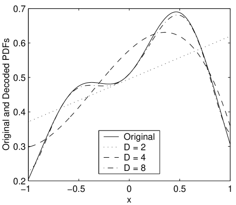
Figure 4: The effect of the dimensionality $D$ on the quality of the neural representation. As $D$ is increased, the decoded PDF more closely matches the original PDF.

2.5 A Neural Integrator Model

An important example of a neural integrator is the group of neurons that maintain the eyes in a fixed position in the absence of visual input. These recurrently connected neurons are able to hold the eye in position for times much longer than the interspike interval of the neurons. Collectively, they form an attractor network that acts as a memory of eye position which lasts for several seconds [Seung, 1996].

By introducing temporal dynamics into the underlying probabilistic models, we can create a model of a neural integrator. The dynamics are straightforward: for a short time $\tau$, the PDF should be unchanged, so

$$\rho(x;t+\tau)=\rho(x;t)$$ (21)

where $x$ is the value (i.e. eye position) stored in the memory.

As discussed above, we generate decoding functions using piecewise-linear activities, linear encoders, and a rectifying activation function. Making use of this representation, the encoding and decoding rules (equations 4 and 5), and the probabilistic dynamics (equation 21), we can show that

$$a_{i}(t+\tau) = g\left(\int\hat{\phi}_{i}(x)\rho(x;t+\tau)dx\right)$$ (22)

$$= g\left(\sum_{j}a_{j}(t)\int\hat{\phi}_{i}(x)\phi_{j}(x)dx\right)$$ (23)

Defining weights

$$\omega_{ij}=\int\hat{\phi}_{i}(x)\phi_{j}(x)dx$$ (24)

we may rewrite this as

$$a_{i}(t+\tau)=g\left(\sum_{j}\omega_{ij}a_{j}(t)\right)$$ (25)

The recurrent neural network that results is fully connected, with each neuron having a synaptic connection to every other neuron.

The stored value of the eye position is extracted by calculating the expectation value of the random variable $x$, weighted by the decoded PDF. Ideally, we would like any value in the supported range to be held constant, so that the network functions as a line attractor [Seung, 1996], a kind of continuous attractor. However, the system actually operates as a collection of point attractors with only a limited number of stable fixed points, as can be seen from the network’s transfer function (Figure 5). The structure of the transfer function, and the number of stable fixed points, depends on the dimensionality $D$ of the minimal space. As the dimensionality of the minimal space is increased, the neural integrator can support additional stable fixed points, eventually approximating a line attractor.

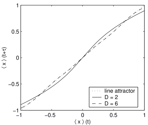
Figure 5: The neural integrator model maintains only a limited number of values, rather than an arbitrary input value. The number of stable fixed points of the neural integrator model can be seen in the network’s transfer function. Here there are two stable fixed points for a neural integrator consisting of 20 neurons with encoders and decoders found using a minimal space with dimension $D=2$. By increasing $D$ to 4, the number of stable fixed points increases to 3 (not shown), while increasing $D$ to 6 yields 4 stable fixed points. With only the 20 neurons of limited precision utilized here, further increases in $D$ do not give rise to further increases in the number of stable fixed points.

This neural integrator model is essentially a variation of the model constructed by Eliasmith and Anderson (1999).

3 Probabilistic Inference Performed by Neural Networks

3.1 Inference

Inference between two related variables $x$ and $y$ in the implicit space is performed by taking a weighted average of the conditional probability $\rho(y\!\mid\!x)$:

$$\rho(y;t+\tau)=\int\rho(y\!\mid\!x)\rho(x;t)dx$$ (26)

We have assumed in equation 26 that the relationship between $x$ and $y$ is independent of the values of the minimal parameters, so

$$\rho(y\!\mid\!x;\left\{A_{\mu}(t)\right\})=\rho(y\!\mid\!x)$$ (27)

This assumption fixes the structure of the probabilistic model, explicitly excluding learning from any neural networks derived from it. The conditional probability $\rho(y\!\mid\!x)$ is like a fixed look-up-table; the Marr-Albus theory of cerebellar function can be directly mapped into equation 26 [Hakimian et al., 1999].

Mapping the implicit-space inference relation 26 into the explicit space of neurons yields a neural network (Anderson, 1994, 1996; Zemel and Dayan, 1997). Specifically, one imposes representations as given in equations 3 and 4 for $x$, and

$$\rho(y;t) = \sum_{j}b_{j}(t)\psi_{j}(y)$$ (28)

$$b_{j}(t) = g\left(\int{\hat{\psi}}_{j}(y)\rho(y;t)dy\right)$$ (29)

for $y$. Then one combines these representations with equation 26, leading to

$$b_{j}(t+\tau)=g\left(\sum_{i}w_{ji}a_{i}(t)\right)$$ (30)

with the coupling coefficients

$$w_{ji}=\int\!\!\!\int{\hat{\psi}}_{j}(y)\rho(y\!\mid\!x)\phi_{i}(x)dxdy$$ (31)

For well-chosen encoding and decoding functions, equations 30 and 31 allow us to construct a neural network that embodies the desired relationship between the implicit variables, without applying a training procedure to find a relation from a data set.

This approach to inference is naturally extended to greater numbers of implicit variables. For example, suppose we add a second input $z$ to the above network, and write

$$\rho(y;t+\tau)=\int\!\!\!\int\rho(y\!\mid\!x,z)\rho(x;t)\rho(z;t)dxdz$$ (32)

Representing $z$ using

$$\rho(z;t) = \sum_{k}c_{k}(t)\theta_{k}(z)$$ (33)

$$c_{k}(t) = f\left(\int{\hat{\theta}}_{k}(z)\rho(z;t)dx\right)$$ (34)

leads to

$$b_{j}(t+\tau)=g\left(\sum_{i}w_{jik}a_{i}(t)c_{k}(t)\right)$$ (35)

with

$$w_{jik}={\int\!\!\!\int\!\!\!\int}{\hat{\psi}}_{j}(y)\rho(y\!\mid\!x,z)\phi_{i}(x)\theta_{k}(z)dxdydz$$ (36)

An interesting feature of this neural network is that it employs multiplicative interactions. This multiplication might be realized by coincidence detection in the dendrites; the implication is that the dendrites are active processing elements [Mel, 1994, Cash and Yuste, 1998].

3.2 A Communication Channel Model

As a concrete example of probabilistic inference within the PDF scheme, we now use equations 30 and 31 to implement a communication channel. Specifically, we wish to encode a single input value $\xi(t)$ into a PDF $\rho(x;t)$ represented by a population of neurons, and copy that PDF into another PDF $\rho(y;t)$ represented by a second population of neurons. To extract a unique output value from $\rho(y;t)$, we focus on the expectation value of $y$. We use 20 neurons to represent the input PDF $\rho(x;t)$ and 16 neurons to represent the output PDF $\rho(y;t)$. The encoders and decoders for these neurons are generated from two straight-line basis functions (Figure 2a) and piecewise-linear neural responses as explained previously (sections 2.2 and 2.3).

Since we only want to encode a single value, and not a complex multimodal distribution, we describe the input using a PDF of the form $\rho(x;t)=\delta(x-\xi(t))$. We set the form of the conditional PDF to be $\rho(y\!\mid\!x)=\delta(y-x)$; accordingly, in the implicit space, we expect that $\rho(y;t)=\delta(y-\xi(t))$. However, a PDF with such a delta-function form is quite intractable in the explicit space—no finite linear combination of functions can yield the expected form of $\rho(y;t)$. Our goal is thus to obtain an accurate estimate of $\xi(t)$, rather than a perfect reconstruction of the PDFs.

To interpret the performance of the neural network, we compare the expectation value $\langle y\rangle$ (weighted by the PDF decoded from the network outputs $\left\{b_{j}(t)\right\}$) to the input $\xi$. The decoded PDF is a weighted sum of linear decoding functions, and is thus a straight line itself. This is of course a poor reproduction of the Dirac delta function input, but $\langle y\rangle$ is closely in accord with the input values (fig 6). We may understand this by considering the basis functions used: they are well-suited for calculating the 0th and 1st moments of the PDF, but unsuitable for calculating higher-order moments.

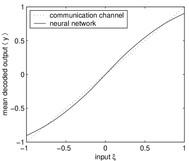
Figure 6: Although the PDF is not accurately represented, the mean value of the PDF can be satisfactorily retrieved from the neural network. By using only two basis functions to generate the decoders, the output PDFs are elements of a space of dimension two. This is suitable for representing the total weight and the mean of a PDF, but not higher moments.

3.3 Working in the Minimal Space

So far, we have used the concept of the minimal space as a tool for developing the encoders and decoders. However, we also can make direct use of the minimal space to set up abstract networks, then convert those into networks of real neurons. To accomplish this, we derive relations between the firing rates in the two spaces ($\left\{A_{\mu}(t)\right\}$ and $\left\{a_{i}(t)\right\}$). The neural network in the explicit space then constitutes a physical implementation of the abstract network in the minimal space. The issues of the role of neuronal firing rate variability in the population code (see for example Abbott and Dayan, 1999) may thus be separated from the issues of the propagation of probabilistic information.

First, consider the decoding rules given by equations 3 and 4. Making use of equation 6, we obtain

$$\sum_{\mu}A_{\mu}(t)\Phi_{\mu}(x)=\sum_{i}a_{i}(t)\sum_{\nu}\kappa_{\nu i}\Phi_{\nu}(x)$$ (37)

Since the $\Phi_{\mu}(x)$ are orthonormal functions, we have

$$A_{\mu}(t)=\sum_{i}\kappa_{\nu i}a_{i}(t)$$ (38)

for transforming from the explicit space to the minimal space.

Next, consider the encoding rule given by equation 5. Recalling that $\hat{\phi}_{i}(x)=\sum_{\nu}\hat{\kappa}_{i\nu}\Phi_{\nu}(x)$ and $A_{\nu}(t)=\int\Phi_{\nu}(x)\rho(x;t)dx$, we have

$$a_{i}(t)=f\left(\sum_{\nu}\hat{\kappa}_{i\nu}A_{\nu}(t)\right)$$ (39)

for transforming from the minimal space to the explicit space.

Using equations 38 and 39, we can translate between the minimal and explicit spaces. This allows us to set up neural networks by first working in the mathematically convenient minimal space. To illustrate this procedure, we return to the $X\longrightarrow Y$ inference network. We take the minimal spaces for both the input $x$ and the output $y$ to be defined by linear functions over the interval $[-1,1]$, with basis functions of the form shown in Figure 2a. The associated PDFs are represented using equation 3 and

$$\rho(y;t)=\sum_{\nu}B_{\nu}(t)\Psi_{\nu}(y)$$ (40)

With these representations, the probabilistic relation given in equation 26 becomes

$$B_{\nu}(t+\tau)=\sum_{\mu}\Omega_{\nu\mu}A_{\mu}(t)$$ (41)

where

$$\Omega_{\nu\mu}=\int\Psi_{\nu}(y)\rho(y\!\mid\!x)\Phi_{\mu}(x)dxdy$$ (42)

We next convert this into a neural network in the explicit space using equations 38 and 39, so that

$$b_{j}(t+\tau) = g\left(\sum_{\nu}\hat{\kappa}^{(y)}_{j\nu}B_{\nu}(t)\right)$$ (43)

$$= g\left(\sum_{i}\sum_{\mu,\nu}\hat{\kappa}^{(y)}_{j\nu}\Omega_{\nu\mu}\kappa^{(x)}_{\mu i}a_{i}(t)\right)$$

By identifying

$$\omega_{ji}=\sum_{\mu,\nu}\hat{\kappa}^{(y)}_{j\nu}\Omega_{\nu\mu}\kappa^{(x)}_{\mu i}$$ (44)

we may rewrite equation 43 as

$$b_{j}(t+\tau)=g\left(\sum_{i}\omega_{ji}a_{i}(t)\right)$$ (45)

arriving at a neural network with the same feedforward dynamics (equation 30) and the same synaptic weights (equation 31) found previously.

This example reproduces results previously found by working in the explicit space, but also highlights several advantages of working in the minimal space. Perhaps most importantly, the fundamental structure of the neural networks is made more transparent by eliminating the redundancies that arise in the networks due to the limited representational ability of neurons. Significantly, we see that computational properties of the nonlinear update rule for the output neurons (equation 43) can be understood by studying the linear update rule in the minimal space (equation 41), consistent with the population vector representations investigated by Georgopoulos et al. (1986).

4 Conclusions

We have examined some of the ramifications of the hypothesis that neural networks represent information as probability density functions. These PDFs are assumed to be expressible a linear combination of some implicit decoding functions, with the decoder for each neuron being weighted by its firing rate. The firing rates in turn may be obtained from a PDF using a complementary set of encoding functions.

In general, the encoding and decoding functions that we have introduced are numerous enough to define spaces of very high dimension, far beyond the range of accurate representation by biological neurons having a precision of only a few bits. To mediate this conflict between computational requirements and biological reality, we have introduced an auxiliary representation of a lower-dimensional minimal space appropriate to the nature and scale of the computations that neurobiological systems actually perform on the relevant input and output analog variables. The basis functions in this minimal space are used to represent both the encoding and decoding functions, limiting the dimensionality of the spaces they define. As an added benefit, the minimal space—and the associated metaneuron variables—can be chosen to have properties that facilitate theoretical characterization of the neural networks resulting from the PDF hypothesis.

These neural networks are based upon the available probabilistic information and upon the encoding and decoding functions. The synaptic weights of the networks are fully specified without a training procedure. A natural extension of the work we have presented is the addition of learning rules for determining the weights. Learning rules would provide several advantages; in particular, they would facilitate the generation of neural networks when data is available but the underlying computations are not entirely clear. The optimization procedure we utilized to find the encoding functions may be a useful starting point for identifying a more complete learning rule.

Researchers in the fields of molecular biology, immunology, genetics, development, and evolution, all of which involve highly complex systems having many degrees of freedom, are beginning to explore the use of “metavariables” as a formal means to reduce the dimensionality of the space of parameters that must be dealt with in achieving viable and tractable quantitative descriptions. The formal results we have derived for metavariable (“metaneuron”) representation of function spaces and the experience we have gained through associated model simulations may prove valuable for parallel investigations in these and other fields.

Returning to the neurobiological context, we may comment on the the role that is envisioned for the PDF formalism in the modeling of brain function. Recent work based on population-temporal coding (e.g. Eliasmith and Anderson 1999, 2002) indicates that the modeling of low-level sensory processing and output motor control do not require such a sophisticated representation; manipulation of mean values is generally sufficient and the representations can be simplified to deal with vector spaces instead of function spaces. However, explicit representation of probabilistic descriptors of the state of knowledge of pertinent analog variables may prove indispensible to an understanding of higher-level processes. For example, estimates of depth at each spatial location from the disparity between the images impinging on both eyes can never be made with precision using a purely bottom-up strategy.

The modern approach to all higher-level image-processing tasks is driven by the theory of Bayesian inference, in which models are developed and parameters estimated based on a set of well-defined rules within a probabilistic framework. In a second paper [Barber et al., 2001], we carry the PDF program a step further by formulating procedures for embedding joint probabilities into neural networks. These procedures allow us to design neural circuit models that pool multiple sources of evidence. In our view, this offers the most rational approach to building and understanding cortical circuits that carry out well-posed information-processing tasks.

References

- [Abbott and Dayan, 1999] Abbott, L. and Dayan, P. (1999). The effect of correlated variability on the accuracy of a population code. Neural Comput., 11(1).
- [Anderson, 1994] Anderson, C. (1994). Basic elements of biological computational systems. International Journal of Modern Physics C, 5(2):135–7.
- [Anderson, 1996] Anderson, C. (1996). Unifying perspectives in neuronal codes and processing. In Ludeña, E., Vashishta, P., and Bishop, R., editors, Condensed Matter Theories, volume 11, pages 365–374, Commack, NY. Nova Science Publishers.
- [Anderson and Abrahams, 1987] Anderson, C. and Abrahams, E. (1987). The Bayes connection. In Proceedings of the IEEE First International Conference on Neural Networks, volume III, pages 105–112, San Diego, CA. IEEE, SOS Print.
- [Anderson and Van Essen, 1987] Anderson, C. and Van Essen, D. (1987). Shifter circuits: a computational strategy for directed visual attention and other dynamic neural processes. Proc. Natl. Acad. Sci. USA, 84(17):6297–6301.
- [Barber et al., 2001] Barber, M., Clark, J., and Anderson, C. (2001). Neural propagation of beliefs. Submitted to Neural Comput., 2001.
- [Bialek and Rieke, 1992] Bialek, W. and Rieke, F. (1992). Reliability and information transmission in spiking neurons. Trends Neurosci., 15(11):428–434.
- [Bialek et al., 1991] Bialek, W., Rieke, F., de Ruyter van Steveninck, R., and Warland, D. (1991). Reading a neural code. Science, 252(5014):1854–1857.
- [Cash and Yuste, 1998] Cash, S. and Yuste, R. (1998). Input summation by cultured pyramidal neurons is linear and position-independent. J. Neurosci., 18(1):10–15.
- [Dayan and Hinton, 1996] Dayan, P. and Hinton, G. (1996). Varieties of Helmholtz machines. Neural Networks, 26:1385–1403.
- [Eliasmith and Anderson, 1999] Eliasmith, C. and Anderson, C. (1999). Developing and applying a toolkit from a general neurocomputational framework. Neurocomputing, 26:1013–1018.
- [Eliasmith and Anderson, 2002] Eliasmith, C. and Anderson, C. (2002). Neural Engineering: The Principles of Neurobiological Simulation. MIT Press.
- [Fuchs et al., 1988] Fuchs, A., Scudder, C., and Kaneko, C. (1988). Discharge patterns and recruitment order of identified motoneurons and internuclear neurons in the monkey abducens nucleus. J Neurophysiol., 60(6):1874–95.
- [Georgopoulos et al., 1986] Georgopoulos, A., Schwartz, A., and Kettner, R. (1986). Neuronal population coding of movement direction. Science, 233(4771):1416–19.
- [Hakimian et al., 1999] Hakimian, S., Anderson, C., and Thach, W. (1999). A PDF model of populations of Purkinje cells. Neurocomputing, 26:169–75.
- [Haykin, 1999] Haykin, S. (1999). Neural Networks: A Comprehensive Foundation. Prentice Hall, Upper Saddle River, NJ, second edition.
- [Hinton and Sejnowski, 1986] Hinton, G. and Sejnowski, T. (1986). Learning and relearning in Boltzmann machines. In Rumelhart, D., McClelland, J., et al., editors, Parallel Distributed Processing: Explorations in Microstructure of Cognition, pages 282–317. MIT Press, Cambridge, MA.
- [Mel, 1994] Mel, B. (1994). Information processing in dendritic trees. Neural Comput., 6:1031–85.
- [Neal, 1992] Neal, R. (1992). Connectionist learning of belief networks. Artificial Intelligence, 56:71–113.
- [Olshausen et al., 1993] Olshausen, B., Anderson, C., and Van Essen, D. (1993). A neurobiological model of visual attention and invariant pattern recognition based on dynamic routing of information. J. Neurosci., 13(11):4700–19.
- [Olshausen et al., 1995] Olshausen, B., Anderson, C., and Van Essen, D. (1995). A multiscale dynamic routing circuit for forming size- and position-invariant object representations. J. Comput. Neurosci., 2(1):45–62.
- [Rieke et al., 1997] Rieke, F., Warland, D., de Ruyter van Steveninck, R., and Bialek, W. (1997). Spikes: Exploring the Neural Code. MIT Press, Cambridge, MA.
- [Salinas and Abbott, 1994] Salinas, E. and Abbott, L. (1994). Vector reconstruction from firing rates. J. Comput. Neurosci., 1(1–2):89–107.
- [Schwartz, 1993] Schwartz, A. (1993). Motor cortical activity during drawing movements: Population representation during sinusoid tracing. J. Neurophysiol., 70(1):28–36.
- [Seung, 1996] Seung, H. (1996). How the brain keeps the eyes still. Proc. Natl. Acad. Sci. USA, 93(23):13339–44.
- [Theunissen et al., 1996] Theunissen, F., Roddey, J., Stufflebeam, S., Clague, H., and Miller, J. (1996). Information theoretic analysis of dynamical encoding by four identified primary sensory interneurons in the cricket cercal system. J. Neurophysiol., 75(4):1345–64.
- [Yang and Zemel, 2000] Yang, Z. and Zemel, R. (2000). Managing uncertainty in cue combination. In Solla, S., Leen, T., and Müller, K., editors, Advances in Neural Information Processing Systems 12, Cambridge, MA. MIT Press.
- [Zemel, 1999] Zemel, R. (1999). Cortical belief networks. In Hecht-Neilsen, R., editor, Theories of Cortical Processing. Springer-Verlag, Berlin.
- [Zemel and Dayan, 1997] Zemel, R. and Dayan, P. (1997). Combining probabilistic population codes. In International Joint Conference on Artificial Intelligence. Morgan Kaufmann.
- [Zemel and Dayan, 1999] Zemel, R. and Dayan, P. (1999). Distributional population codes and multiple motion models. In Kearns, M., Solla, S., and Cohn, D., editors, Advances in Neural Information Processing Systems 11, Cambridge, MA. MIT Press.
- [Zemel et al., 1998] Zemel, R., Dayan, P., and Pouget, A. (1998). Probabilistic interpretation of population codes. Neural Comput., 10(2):403–30.