Electron Spin Resonance in $S=1/2$ antiferromagnetic chains

Abstract

A systematic field-theory approach to Electron Spin Resonance (ESR) in the $S=1/2$ quantum antiferromagnetic chain at low temperature $T$ (compared to the exchange coupling $J$) is developed. In particular, effects of a transverse staggered field $h$ and an exchange anisotropy (including a dipolar interaction) $\delta$ on the ESR lineshape are discussed. In the lowest order of perturbation theory, the linewidth is given as $\propto Jh^{2}/T^{2}$ and $\propto(\delta/J)^{2}T$, respectively. In the case of a transverse staggered field, the perturbative expansion diverges at lower temperature; non-perturbative effects at very low temperature are discussed using exact results on the sine-Gordon field theory. We also compare our field-theory results with the predictions of Kubo-Tomita theory for the high-temperature regime, and discuss the crossover between the two regimes. It is argued that a naive application of the standard Kubo-Tomita theory to the Dzyaloshinskii-Moriya interaction gives an incorrect result. A rigorous and exact identity on the polarization dependence is derived for certain class of anisotropy, and compared with the field-theory results.

I Introduction

Quantum spin chains have been studied extensively for both their experimental and theoretical interests. Among many experimental methods of investigation, Electron Spin Resonance (ESR) is unique for its high sensitivity to anisotropy. While the theory of ESR has been studied[1, 2, 3, 4] for a long time, there remain important open problems, especially for strongly interacting systems. One of the problems is that, generally one has to make a crucial assumption about the lineshape at some point during the calculation. As we will demonstrate, such an assumption could be incorrect in some cases although it might have been taken for granted in the literature. In addition, in an actual calculation one has to calculate various correlation functions. Traditionally, crude approximations such as the high-temperature approximation, the classical spin approximation and the decoupling of the correlation functions are used. However, these approximations break down when the many-body correlation effects are strong. As a consequence, rather little has been understood about ESR when many-body correlations become important. Even in the cases which were believed to be understood with the existing theories, there appear to be subtle problems.

In this paper, we study ESR in $S=1/2$ quantum spin chains in the “one-dimensional critical region” where the temperature $T$ is sufficiently small compared to the characteristic energy of the exchange interaction $J$ (but $T$ is still large compared to three-dimensional ordering temperature or spin-Peierls transition temperature.) We stress that ESR in such a region is essentially a many-body problem. Here, many of the traditional theoretical techniques lose their validity. Instead, $(1+1)$-dimensional field theory should describe the universal, low-energy/large-distance behavior. Our main purpose in the present paper is to develop a new approach to ESR based on field theory (bosonization) methods. At least for several simple cases (which are of experimental interest) we are able to formulate the problem in terms of the systematic Feynman-Dyson perturbation theory, avoiding previously made ad hoc assumptions. We will study several consequences of our theory for two types of perturbations of the one-dimensional $S=1/2$ Heisenberg antiferromagnet: a staggered field, and an exchange anisotropy (or dipolar interaction). When the effect of the anisotropy is small, the ESR lineshape is shown to be Lorentzian up to a possible small smooth background; the width and the shift of the Lorentzian peak are given perturbatively. In one dimension, it was argued that the diffusive spin dynamics leads to a non-Lorentzian lineshape, which is indeed observed in the $S=5/2$ antiferromagnetic chain TMMC[4]. However, our results imply that the argument does not apply to the present case of the $S=1/2$ antiferromagnetic chain at low temperature.

In a compound with a low crystal symmetry permitting a staggered component of the gyromagnetic tensor or a staggered Dzyaloshinskii-Moriya (DM) interaction, an effective staggered field is also produced by the applied uniform field. The staggered field corresponds to a relevant operator in the Renormalization Group sense, and is related to the field-induced gap phenomenon recently found in several quasi-one dimensional $S=1/2$ antiferromagnets[5, 6, 8, 9]. Since it is a relevant operator, one may expect that its effect is enhanced at lower temperatures. Indeed, we find that the staggered field contributes to the linewidth proportionally to $h^{2}/T^{2}$ where $h$ is the magnitude of the staggered field. We propose this as an explanation of the peculiar low-temperature behavior[10] found in ESR on Cu Benzoate nearly 30 years ago. Moreover, we propose that the sharp resonance found at very low temperature[11], which was understood as a signature of a three-dimensional Néel ordering, may well be understood in a purely one-dimensional framework based on sine-Gordon field theory.

On the other hand, dipolar interactions or exchange anisotropies are present in virtually any real material. We find that their contribution to the linewidth is proportional to $T$, which appears to be consistent with existing experimental data on several quasi one dimensional $S=1/2$ antiferromagnet such as CuGeO₃, KCuF₃ and NaV₂O₅.

Basic ideas and some of the results in the present paper were presented briefly in Ref. [12]. This paper is organized as follows. In Section II, we briefly review the basics of ESR in interacting spin systems, including a few (apparently) new results, namely an exact and rigorous identity on the polarization dependence, and the relation between the Kubo-Tomita[1] and the Mori-Kawasaki[2, 3] theories. In Sections III and  V we develop a new framework for studying ESR in quantum spin chains, based on field theory methods and, in particular, the Dyson formula expressing the Green’s function for a scalar field in terms of the self-energy. It is applied in Sections IV, VI, VII and  VIII to systems with an exchange anisotropy (or dipolar interaction) or a transverse staggered field. (The case of an exchange anisotropy with the axis parallel to the field turns out to be easier to treat and not to require the self-energy formalism. Therefore it is treated first, in Section IV.) In Section IX, we compare our results to those in the high-temperature regime obtained with the previous approach. Section X is devoted to conclusions. Appendix A contains an alternative derivation of an old formula for the width/shift first derived by Mori and Kawasaki [2, 3].

II Electron Spin Resonance

A Definition of the problem

A single spin in a magnetic field $H$ has energy levels separated by the Zeeman energy $E_{Z}=g\mu_{B}H$. If an electromagnetic wave of angular frequency $\omega$ is applied to such a system, resonant absorption occurs when $\hbar\omega=E_{Z}$ and the polarization (direction of the oscillating magnetic field) is perpendicular to the static field. When the spins are coupled by interactions, the physics is of course not that simple. However, generally some resonant absorption occurs also in the interacting system. This is the phenomenon of ESR which we study in the present paper. In an interacting system, it is also possible to observe absorption of the electromagnetic wave polarized parallel to the static magnetic field (so called Voigt configuration.) In this paper, we focus on the standard (Faraday) configuration, which measures the absorption of the electromagnetic wave polarized perpendicular to the static magnetic field.

Assuming that the absorption can be described by linear response theory, the absorption intensity $I(\omega)$ per volume for the radiation linearly polarized in the $\alpha\perp z$ direction is given by

$$I(\omega)=\frac{{H_{R}}^{2}\omega}{2}\chi^{\prime\prime}_{\alpha\alpha}(q=0,\omega),$$ (1)

where $H_{R}$ is the amplitude of the radiation and $\chi^{\prime\prime}$ is the imaginary part of the dynamical magnetic susceptibility. $\chi^{\prime\prime}$ is related to the retarded Green’s function ${\cal G}^{R}$ as

$$\chi^{\prime\prime}_{\alpha\beta}(q,\omega)=-{\rm Im}{\cal G}^{R}_{\alpha\beta}(q,\omega),$$ (2)

where ${\cal G}^{R}_{\alpha\beta}$ is defined by

$${\cal G}^{R}_{\alpha\beta}(q,\omega)=-i\int_{0}^{\infty}dt\sum_{x}\langle[S^{\alpha}(x,t),S^{\beta}(0,0)]\rangle e^{-iqx+i\omega t}$$ (3)

where $\langle\ldots\rangle$ is the statistical average at temperature $T$. In most experiments, the applied electromagnetic wave is typically in the microwave regime, and its wavelength is very large compared to all relevant length scales in the antiferromagnet since the spin-wave velocity is much less than the speed of light. Thus, in ESR, the dynamical susceptibility is measured at essentially zero momentum $q=0$. ESR probes the dynamics of the system only at the special momentum $q=0$, in contrast to neutron scattering which can be used to scan momentum space. However, as we will explain below, there is an interesting feature at the special momentum $q=0$. Together with the relatively easy availability of highly precise data, ESR offers a unique insight into magnetic systems which would be difficult to obtain with other experimental methods.

A remarkable feature of ESR is that, if the Hamiltonian of the system (apart from the Zeeman term) is isotropic (ie. $SU(2)$ symmetric), the resonance is still at the Zeeman energy and completely sharp, as if there is no interaction at all. This result can be deduced rather easily from the equation of motion, as we will show in the following. Throughout this paper, we take the direction of the static applied field as the $z$-axis. Let us consider the total Hamiltonian

$${\cal H}={\cal H}_{0}+{\cal H}_{Z},$$ (4)

where ${\cal H}_{Z}=-H\sum_{j}S^{z}_{j}$ is the Zeeman term and ${\cal H}_{0}$ is the exchange Hamiltonian which is assumed to be $SU(2)$ symmetric. We choose units so that $\hbar=g\mu_{B}=1$ except where explicitly mentioned otherwise; these constants can be recovered by dimensional analysis. We also assume $H$ is much smaller than the exchange coupling $J$ (ie. energy scale of ${\cal H}_{0}$). As we have mentioned above, in ESR the electromagnetic wave is coupled to the $q=0$ component of the spin operators, namely the total spin operators $S^{\alpha}=\sum_{j}S^{\alpha}_{j}$. The Heisenberg equation of motion for $S^{+}=S^{x}+iS^{y}$ reads

$$\frac{dS^{+}}{dt}=i[{\cal H},S^{+}]=i[{\cal H}_{Z},S^{+}]=-iHS^{+},$$ (5)

because ${\cal H}_{0}$ commutes with $S^{+}$ due to the $SU(2)$ symmetry of ${\cal H}_{0}$. It follows that $S^{+}(t)=S^{+}e^{-iHt}$, and consequently $\chi^{+-}(0,\omega)\propto\delta(\omega-H)$. This means that the resonance is completely sharp, and located exactly at the Zeeman energy. Namely, this resonance has the lineshape identical to ESR in a single (non-interacting) spin in spite of an arbitrary strong exchange interaction. On the other hand, the absorption intensity is generally affected by the exchange interaction ${\cal H}_{0}$. For example, in a spin-gap system at zero temperature, the absorption intensity is zero if the applied field $H$ is smaller than the gap.

As we have seen, the completely sharp resonance is related to the $SU(2)$ symmetry of the exchange Hamiltonian ${\cal H}_{0}$. While it is natural that symmetries of the system are important in determining the dynamics of the system, the present situation is rather unique, for the $SU(2)$ symmetry is explicitly broken down to $U(1)$ by the applied static field but is still essential in ESR. This peculiar feature is related to the fact that the applied field couples to the total magnetization $S^{z}=\sum_{j}S^{z}_{j}$, which is a generator of the global $SU(2)$ symmetry and is conserved under ${\cal H}_{0}$. Since the total magnetization and Hamiltonian are simultaneously diagonalizable, the applied field does not change the eigenstates of the system, if they are classified by $S^{z}$. The only effect of the static applied field is to shift the energy levels of the eigenstates; the shifted energy levels still reflects the $SU(2)$ multiplet structure. This kind of “weak” symmetry breaking by one of the symmetry generators preserves some structures of the fully symmetric system. In ESR of an isotropic system ${\cal H}_{0}$, the $SU(2)$ symmetry is only weakly broken and is essential in determining the ESR spectrum.

A similar application of the concept of weakly broken global symmetry was also exploited recently by S. C. Zhang[13] in his $SO(5)$ theory of high-$T_{c}$ superconductivity. Namely, in the $SO(5)$ theory, the most important terms in the effective Hamiltonian are $SO(5)$ symmetric one and the chemical potential couples to one of the generators of the global $SO(5)$ symmetry. The so-called $\pi$-excitation in this context is a sharp resonance which is similar to ESR in isotropic spin systems.

In real magnetic systems, there are various types of anisotropy, such as the dipolar interaction. Let us write the total Hamiltonian as

$${\cal H}={\cal H}_{0}+{\cal H}^{\prime}+{\cal H}_{Z},$$ (6)

where ${\cal H}^{\prime}$ is the symmetry-breaking perturbation. Throughout this paper, we assume the interaction to be nearly isotropic, namely that ${\cal H}^{\prime}$ is small compared to the other terms ${\cal H}_{0}$ and ${\cal H}_{Z}$. Once the perturbation ${\cal H}^{\prime}$ is added, the argument leading to the delta-function resonance at the Zeeman energy breaks down. Thus, in general, the addition of ${\cal H}^{\prime}$ causes changes in the lineshape, such as a broadening and a shift of the resonance. The main theoretical problem is then to calculate the absorption spectrum for the given Hamiltonian ${\cal H}$ and other conditions such as the temperature of the system.

B Previous theories

The existing approaches to ESR, such as those of Kubo and Tomita [1] and of Mori and Kawasaki [2, 3] were developed mainly during 1950s-60s. Here we summarize briefly, a part of those achievements which is closely related to our analysis.

When the isotropic exchange interactions between spins are weak, namely ${\cal H}_{0}$ is much smaller than ${\cal H}_{Z}$, the lineshape is generally expected to be Gaussian. On the other hand, once the anisotropy ${\cal H}^{\prime}$ is present, strong isotropic exchange interactions ${\cal H}_{0}$ between spins affects the ESR lineshape, even though it does not break the $SU(2)$ symmetry by itself. In the presence of the strong interaction (${\cal H}_{0}\gg{\cal H}_{Z}$), which applies to the problem considered in this paper, the lineshape is generally expected to be Lorentzian. (On the other hand, the lineshape is believed to be neither Gaussian nor Lorentzian, when the spin diffusion is dominant. [4]) The effect of the isotropic exchange interactions on the lineshape has been traditionally called Exchange Narrowing. We emphasize that ESR in such an interacting spin system probes the collective motion of the many-body system. In this paper, we focus on this limit of strong isotropic exchange interaction, while other cases have been discussed previously as well [1, 2, 3].

For the case of the Lorentzian lineshape, Mori and Kawasaki[2] proposed a formula, which we call the MK formula, for the linewidth $\eta$:

$$\eta=\frac{1}{2\chi_{u}H}{\rm Im}{[-G^{R}_{{\cal A}{\cal A}^{\dagger}}(\omega=H)]},$$ (7)

where $\chi_{u}$ is the magnetic susceptibility and $G^{R}_{{\cal A}{\cal A}^{\dagger}}(\omega)$ is the Fourier transform of the unperturbed retarded Green’s function

$$G^{R}_{{\cal A}{\cal A}^{\dagger}}(t)=-i\theta(t)\langle[{\cal A}(t),{\cal A}^{\dagger}(0)]\rangle_{0},$$ (8)

where $\langle\ldots\rangle_{0}$ is the expectation value under the unperturbed Hamiltonian ${\cal H}_{0}+{\cal H}_{Z}$, $\theta(t)$ is the step function, and ${\cal A}$ is defined by the commutator

$${\cal A}=[{\cal H}^{\prime},S^{+}].$$ (9)

In this paper, ${\cal G}$ refers to a full Green’s function calculated using the Hamiltonian including the perturbation ${\cal H}^{\prime}$, while $G$ denotes the unperturbed Green’s function evaluated in the absence of the perturbation. Both kinds of Green’s functions (${\cal G}$ and $G$) should be evaluated including the Zeeman term ${\cal H}_{Z}$, in the original spin chain context. However, as we will see in Section III, in the effective field theory, the Zeeman term is absorbed by a momentum shift. Thus, the Green’s functions in the effective field theory will be defined without explicitly including the Zeeman term.

In addition to the broadening, the perturbation ${\cal H}^{\prime}$ also causes a shift of the resonance energy; the shift is given by

$$\Delta\omega=\frac{-1}{2\chi_{u}H}\left\{\langle[{\cal A},S^{-}]\rangle-{\rm Re}G^{R}_{{\cal A}{\cal A}^{\dagger}}(\omega=H)\right\}.$$ (10)

This formula for the shift is slightly different from the one given in the original paper[2]. We believe that ours is the correct one in the lowest order of perturbation theory.

The derivation of the MK formulae in the original paper seems somewhat involved, and it is not clear to us what assumptions are necessary to prove them. However, we found that the MK formulae is indeed exact in the lowest order of the perturbation theory, if the (single) Lorentzian lineshape is assumed. Explicitly speaking, we must assume:

$${\cal G}^{R}_{S^{+}S^{-}}(\omega)=\frac{2\langle S^{z}\rangle}{\omega-H-\Sigma},$$ (11)

where $\Sigma$ is a smooth function of $\omega$ near $\omega=H$. Regarding $\Sigma$ as a constant near the resonance, we obtain a Lorentzian line-shape. [Setting $\Sigma=0$ in Eq. (11) gives the exact result for the isotropic case ${\cal H}^{\prime}=0$.] The simple, and possibly new, alternative derivation using the equation of motion is presented in Appendix A.

On the other hand, Kubo and Tomita[1] studied ESR using a somewhat different formulation. For the case of Lorentzian lineshape, their theory gives the following formula for the linewidth, at high temperature:

$$\eta\sim\frac{1}{|J|}\frac{\langle{\cal A}{\cal A}^{\dagger}\rangle}{\langle S^{+}S^{-}\rangle},$$ (12)

where the expectation value is the static correlation function. We shall call this the KT formula in this paper. We could not find in the literature how the two formulae (7) and (12) are related. On the other hand, if the KT formula (12) for the Lorentzian lineshape is indeed valid at high temperature, it must be consistent with the MK formula. In fact, we have verified that the KT formula (12) follows from the high-temperature limit of the MK formula (7) with a certain assumption. The derivation is given as follows. Taking the Fourier transform of eq. (8), at temperature $T$,

$$G^{R}_{{\cal A}{\cal A}^{\dagger}}(\omega)=-\frac{i}{Z}\int_{0}^{\infty}dte^{i\omega t}{\rm Tr}{\left([{\cal A}(t),{\cal A}^{\dagger}(0)]e^{-({\cal H}_{0}+{\cal H}_{Z})/T}\right)},$$ (13)

where $Z={\rm Tr}{e^{-({\cal H}_{0}+{\cal H}_{Z})/T}}$. Expanding this up to the first order in $1/T$, we find,

$$G^{R}_{\cal A{\cal A}^{\dagger}}(\omega) \sim \frac{i}{TZ_{\infty}}\int_{0}^{\infty}dt{\rm Tr}{\left([{\cal H}_{0}+{\cal H}_{Z},{\cal A}(t)]{\cal A}^{\dagger}(0)\right)}e^{i\omega t}$$ (14)

$$= \frac{1}{TZ_{\infty}}\int_{0}^{\infty}dt{\rm Tr}{\left(\frac{d{\cal A}}{dt}(t){\cal A}^{\dagger}(0)\right)}e^{i\omega t}$$ (15)

$$= -\frac{1}{TZ_{\infty}}{\rm Tr}\left[{{\cal A}(0){\cal A}^{\dagger}(0)}\right]-i\frac{\omega}{TZ_{\infty}}\int_{0}^{\infty}dt{\rm Tr}\left[{{\cal A}(t){\cal A}^{\dagger}(0)}\right]e^{i\omega t},$$ (16)

where the time evolution is defined with respect to the unperturbed Hamiltonian ${\cal H}_{0}+{\cal H}_{Z}$ and $Z_{\infty}={\rm Tr}1$ is the partition function in the infinite temperature limit. The first term is real and does not contribute to the imaginary part. If we assume that the dynamical correlation function at infinite temperature ${\rm Tr}\left[{{\cal A}^{\dagger}(t){\cal A}(0)}\right]$ decays exponentially with the characteristic time $\tau_{c}\sim 1/J$, the second term gives $-i\frac{\omega}{JT}\langle{{\cal A}^{\dagger}(0){\cal A}(0)}\rangle_{\infty}$, where $\langle\rangle_{\infty}$ is the expectation value at the infinite temperature and we use $\omega\ll J$. We note that a similar assumption was made also in the original derivation of eq. (12) in the Kubo-Tomita paper. Thus the MK formula (7) reduces, in the high-temperature limit, to

$$\eta\sim\frac{\langle{\cal A}{\cal A}^{\dagger}\rangle_{\infty}}{2\chi_{u}TJ}.$$ (17)

Because $\langle S^{+}S^{-}\rangle\sim 2\chi_{u}T$ in the high-temperature limit, this is equivalent to the KT formula (12). We note that, because $\tau_{c}\sim 1/J$ is valid only as an order-of-magnitude estimate at best, the KT formula has the uncertainty of an overall constant factor.

Recently, a numerical approach to ESR in quantum spin chains is also being developed[14] by a direct calculation of the dynamical susceptibility $\chi^{\prime\prime}(\omega)$. Since it is based on an exact diagonalization of the full spectrum of short chains, it is restricted to rather short chain of up to 10 spins even for $S=1/2$, making finite size effects rather severe. On the other hand, the direct numerical calculation is applicable at any temperature. In contrast, the field theory approach, which we will develop in the present paper, is valid only at low temperatures while it is based on the thermodynamic limit. Thus they are complementary to each other.

We remark that some results quite closely related to ours were derived by Giamarchi and Millis[30, 31] in their work on the ac conductivity of a Tomonaga-Luttinger (TL) liquid. We will comment on the connections with our work later.

C Polarization dependence

When observing ESR in the Faraday configuration, the polarization of the electromagnetic wave is perpendicular to the direction of the static magnetic field, which we take as the $z$-axis. There are still two independent possible polarizations; the linear polarization can take any direction in the $xy$-plane. Except when the total Hamiltonian ${\cal H}$ is invariant under a rotation about the $z$ axis, the absorption spectrum generally depends on the polarization. Within the linear response theory, the dependence comes from the difference between the dynamical susceptibility $\chi^{\prime\prime}_{xx}(0,\omega)\neq\chi^{\prime\prime}_{yy}(0,\omega)$. The MK formula ignores the possible polarization dependence, because it deals with $\chi^{\prime\prime}_{+-}\sim\chi^{\prime\prime}_{xx}+\chi^{\prime\prime}_{yy}$, and not $\chi^{\prime\prime}_{xx}$ and $\chi^{\prime\prime}_{yy}$ separately. The polarization dependence was discussed theoretically first by Natsume et al. [15, 16, 17] generalizing the Kubo-Tomita theory. It has also been observed experimentally [15, 16] and numerically [14].

However, apparently it has been not recognized that, for some special cases, an exact and rigorous result on the polarization dependence can be derived easily from the equation of motion. Let us consider the special case in which the perturbation ${\cal H}^{\prime}$ is written in terms of the $x$ component of the spin operator $S^{x}_{j}$. The examples include the transverse staggered field ${\cal H}^{\prime}=h\sum_{j}(-1)^{j}S^{x}_{j}$, and the exchange anisotropy with the anisotropy axis in the $x$ direction ${\cal H}^{\prime}=\delta\sum_{j}S^{x}_{j}S^{x}_{j+1}$. In these cases, $[S^{x},{\cal H}^{\prime}]=0$ holds, and consequently

$$\frac{dS^{x}}{dt}=HS^{y}.$$ (18)

This identity leads to

$$\chi^{\prime\prime}_{xx}(0,\omega)=\frac{H^{2}}{\omega^{2}}\chi^{\prime\prime}_{yy}(0,\omega),$$ (19)

and more generally, for the polarization in the direction $\alpha$ in the $xy$-plane,

$$\chi^{\alpha\alpha}(0,\omega)=\frac{H^{2}\cos^{2}{\Phi}+\omega^{2}\sin^{2}{\Phi}}{\omega^{2}}\chi^{yy}(0,\omega),$$ (20)

where $\Phi$ is the angle between $x$ and $\alpha$. (In the notation of Refs. [15, 16, 17], $\theta=90$ degree and their $\phi$ corresponds to our $\Phi$.)

For a sharp resonance concentrated near $\omega\sim H$, the polarization dependence is not significant. However, if the center of the resonance is defined by the average frequency of the spectrum

$$\bar{\omega}_{\alpha}=\frac{\int\omega I_{\alpha}(\omega)d\omega}{\int I_{\alpha}(\omega)d\omega},$$ (21)

$\bar{\omega}_{x}<\bar{\omega}_{y}$ because the higher frequency part is emphasized in the latter. As a consequence, there is a positive frequency shift for the polarization in $y$ axis, compared to the case where in $x$ axis.

This is in agreement with theoretical and experimental results in Refs. [15, 16] and numerical results in Ref. [14], on the exchange anisotropy. We note that, in the actual experiments on ESR, the resonance frequency is kept fixed and the applied field is scanned to measure the absorption. Because of this, it is customary to discuss the shift of the resonance field for a fixed frequency. The direction (positive or negative) of the field shift is opposite to that of the frequency shift we discuss in this paper. They find that the resonance field is shifted negatively for the polarization in $y$ direction compared to the $x$ polarization case, which is indeed consistent with our result. The angular dependence is also consistent with the theoretical formula in Ref. [15]. On the other hand, in Ref. [17], the polarization dependence is studied by a different formalism (Mori’s memory function method.) When the anisotropy axis is perpendicular to the applied field, the obtained polarization dependence is rather opposite to the above, and is in contradiction to our rigorous result (19).

III Field-theory approach to the $S=1/2$ Heisenberg antiferromagnetic chain

A Bosonization of $S=1/2$ Heisenberg chain

In the present paper, we mainly discuss ESR on the one-dimensional $S=1/2$ Heisenberg antiferromagnet

$${\cal H}_{0}=J\sum_{j}\vec{S}_{j}\cdot\vec{S}_{j+1}.$$ (22)

with symmetry-breaking perturbation ${\cal H}^{\prime}$ and of course the Zeeman term ${\cal H}_{Z}$. The low-energy physics of the one-dimensional quantum antiferromagnets is well described by field theory methods (bosonization). In this section, we briefly summarize the aspects of this approach that are relevant to the present discussion of the ESR. We refer the reader to Refs. [18, 19] for more details. While the method is now standard, here we also clarify subtleties specific to ESR problems, which are related to the weakly broken $SU(2)$ symmetry discussed in Section II.

The effective field theory of the $S=1/2$ Heisenberg chain ${\cal H}_{0}$ is given by the free boson Lagrangian

$${\cal L}=\frac{1}{2}\left[(\partial_{0}\phi)^{2}-(\partial_{1}\phi)^{2}\right],$$ (23)

where $x^{0}=vt$, $x^{1}=x$ and we make identification $\phi\sim\phi+2\pi R$ with the compactification radius $R$. The radius $R$ is actually fixed to the value $1/\sqrt{2\pi}$ by the $SU(2)$ symmetry. Hereafter we set $v=1$ for simplicity; the spinon velocity $v$ can be recovered by dimensional analysis when necessary.

At zero uniform field, the spin operators may be written in terms of the field $\phi$ as follows:

$$S^{z}_{j} \sim \frac{1}{2\pi R}\frac{\partial\phi}{\partial x}+C_{s}^{z}(-1)^{j}\cos{\frac{\phi}{R}}$$ (24)

$$S^{-}_{j} \sim C_{u}^{-}e^{-i2\pi R\tilde{\phi}}\cos{\frac{\phi}{R}}+C^{-}_{s}(-1)^{j}e^{-i2\pi R\tilde{\phi}},$$ (25)

where the dual field $\tilde{\phi}$ is defined in terms of right-mover $\varphi_{R}$ and $\varphi_{L}$ as $\phi=\varphi_{R}+\varphi_{L}$ and $\tilde{\phi}=\varphi_{R}-\varphi_{L}$. While $S^{z}$ and $S^{x,y}$ are represented in a very different way, their correlation functions turn out to be equal at the $SU(2)$ invariant radius $R=1/\sqrt{2\pi}$, as required from the symmetry of the original Heisenberg chain.

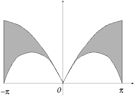
FIG. 1.: The spin structure factor of the $S=1/2$ Heisenberg antiferromagnetic chain at $T=0$. It is non-vanishing only in the filled region shown in the frequency-momentum plane. The structure factor becomes a delta function $\delta(\omega-vq)$ in the $q\rightarrow 0$ limit.

The dynamical structure factor ${\cal S}^{\alpha\alpha}$ (Fourier transformation of the spin correlation function) of the Heisenberg chain has been studied in detail. It is equivalent to the dynamical susceptibility for $T=0$ and $\omega>0$. At zero temperature, the dynamical structure factor is non-vanishing only in the limited region of the frequency $\omega$ – momentum $q$ space shown in Fig. 1. The field theory actually can handle only the low-energy excitations near momentum $0$ and $\pi$. The structure factor for ${\cal S}^{zz}$ near $q=0$ and $q=\pi$ is given by the correlation function of $\partial\phi/\partial x$ and $\cos{(\phi/R)}$ respectively. At $T=0$, they read

$${\cal S}^{zz}(\omega,q)\propto\delta(\omega-|q|)\theta(\omega)$$ (26)

for $q\sim 0$ and

$${\cal S}^{zz}(\omega,q)\propto\frac{1}{\sqrt{\omega^{2}-(q-\pi)^{2}}}\theta(\omega-|q-\pi|)$$ (27)

for $q\sim\pi$. It is noted that the structure factor is completely sharp and is delta-function like at $q\sim 0$. In fact, the structure factor at $q\sim 0$ remains so even at finite temperature. As mentioned before, the structure factor is of course isotropic (${\cal S}^{xx}={\cal S}^{yy}={\cal S}^{zz}$) at $H=0$ for the isotropic Heisenberg chain.

Now let us consider the effect of the applied magnetic field. The Zeeman term ${\cal H}_{Z}$ in the Lagrangian becomes, upon bosonization,

$${\cal L}_{H}={H\over\sqrt{2\pi}}{\partial\phi\over\partial x}.$$ (28)

This term can be eliminated by a redefinition of the boson field

$$\phi(t,x)\to\phi(t,x)+{H\over\sqrt{2\pi}}x.$$ (29)

but $\tilde{\phi}$ remains unchanged. This is equivalent to the shift of chiral fields as

$$\varphi_{R}\rightarrow\varphi_{R}+\frac{1}{2\sqrt{2\pi}}Hx,\varphi_{L}\rightarrow\varphi_{L}+\frac{1}{2\sqrt{2\pi}}Hx.$$ (30)

While this leaves the free Lagrangian unchanged, it does change the bosonization formulae of physical spin operators:

$$S^{z} \sim m+\frac{1}{2\pi R}\frac{\partial\phi}{\partial x}+C_{s}^{z}\cos{[\frac{\phi}{R}+(H+\pi)x]},$$ (31)

$$S^{\pm} \sim C_{u}^{-}e^{-i\sqrt{2\pi}\tilde{\phi}}\cos{(\frac{\phi}{R}+Hx)}+C^{-}_{s}(-1)^{j}e^{-i2\pi R\tilde{\phi}}.$$ (32)

The first term $m$ in $S^{z}$ represents the expectation value of the magnetization induced by the magnetic field $H$. For a small magnetic field, $m$ is proportional to the field $H$. Another important feature is that the applied field induces the shift of the soft-mode momentum[20, 21]. The shift occur differently for the longitudinal ($z$) and the transverse ($x,y$) components. The gapless points under the applied uniform field $H$ are at $q=0$ (uniform part) and $q=\pi\pm H$ (“staggered” part) for the longitudinal modes. For the transverse modes, they are at $q=\pm H$ (“uniform” part) and $q=\pi$ (staggered part.)

Let us focus on the transverse mode near $q=0$, because the transverse mode at $q=0$ is measured in ESR in the Faraday configuration. For simplicity, here we restrict ourselves to zero temperature. In the low energy effective theory, the “uniform” part of the $S^{\pm}$ is given

$$S^{\pm}\propto e^{\pm(iHx+i\sqrt{8\pi}\phi_{R})}+e^{\mp(iHx+i\sqrt{8\pi}\phi_{L})},$$ (33)

where we have used the $SU(2)$ symmetric compactification radius $R=1/\sqrt{2\pi}$ (see below for reason for taking this value.) This gives the correlation function of $S^{\pm}$ at zero temperature:

$$\langle S^{+}(t,x)S^{-}(0,0)\rangle\propto{e^{iHx}\over(t-i\epsilon+x)^{2}}+{e^{-iHx}\over(t-i\epsilon-x)^{2}}$$ (34)

Dynamical structure factor $S_{+-}$, which is the Fourier transform of the above is,

$$S_{+-}(\omega,q) \propto \int_{-\infty}^{\infty}dt\int_{-\infty}^{\infty}dxe^{i(\omega t-qx)}\left[{e^{iHx}\over(t-i\epsilon+x)^{2}}+{e^{-iHx}\over(t-i\epsilon-x)^{2}}\right]$$ (35)

$$= \int_{-\infty}^{\infty}dx[-2\pi\omega\theta(\omega)]e^{-iqx}\left[e^{iHx-i\omega x}+e^{-iHx+i\omega x}\right]$$ (36)

$$\propto \omega\theta(\omega)[\delta(\omega-H+q)+\delta(\omega-H-q)].$$ (37)

The other one $S_{-+}$ is given by replacing $H\rightarrow-H$ in the above, using the time reversal transformation. Thus

$$S_{-+}(\omega,q)\propto\omega\theta(\omega)[\delta(\omega+H+q)+\delta(\omega+H-q)].$$ (38)

Namely, $S_{+-}$ and $S_{-+}$ give different branches of excitation. The fact that $S_{-+}$ does not contain the branch (37) was recognized earlier (see Fig. 17 of Ref. [21].) On the other hand, that $S_{+-}$ lacks the branch (38) (at least in the low-energy limit) was apparently not appreciated in Fig. 18 of Ref. [21]. $S_{xx}$ and $S_{yy}$ are given by their superposition

$$S_{xx}(\omega,q)=S_{yy}(\omega,q)\propto\omega[\delta(\omega-|q+H|)+\delta(\omega-|q-H|)].$$ (39)

This zero-temperature transverse structure factor near $q=0$ under the applied magnetic field is shown in Fig. 2. Because the structure factor near $q=0$ was sharp, and the gapless point is shifted by $H$, we expect a sharp resonance at energy $\omega\sim H$ at $q=0$. This corresponds to the expected paramagnetic ESR for the isotropic Heisenberg chain.

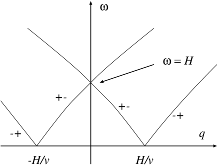
FIG. 2.: The zero temperature transverse spin structure factor $S_{xx}(\omega,q)=S_{yy}(\omega,q)$ of the $S=1/2$ Heisenberg antiferromagnetic chain under an applied field $H$, near $q=0$. It is approximately proportional to $\omega[\delta(\omega-|q-H|)+\delta(\omega-|q+H|)]$, giving the resonance at $q=0,\omega=H$. This consists of two branches coming from $S_{+-}$ and $S_{-+}$, which are marked by $+-$ and $-+$ in the graph. In fact, there is a small spreading of the spectrum and the structure factor is generally not a perfect delta function. However, it is exactly the delta function $\delta(\omega-H)$ at $q=0$, as explained in the text.

However, it should be noted that we have so far ignored various renormalization effects due to the applied magnetic field. There are irrelevant operators, which themselves vanish in the low-energy limit but renormalize parameters of the low-energy effective theory. The way they renormalize is affected by the applied magnetic field. In general, the precise value of the momentum shift is given by $2\pi m$ rather than $H$, where $m$ is the magnetization. This can be derived from the shift of Fermi momentum in the Jordan-Wigner transformation, and also is required from a rigorous version of Luttinger’s theorem in one dimension[22]. Restoring the spinon velocity $v$, the ESR frequency appears to be given by $2\pi mv$. For the standard Heisenberg antiferromagnetic chain in an applied field, the magnetization $m$ and the spinon velocity $v$ can be obtained as a function of $H$ from the Bethe Ansatz integral equation. Generally, $2\pi mv$ is different from $H$ except in the zero field limit, implying that the ESR frequency deviates from $H$. However, this cannot be true, because the equation of motion for the original Heisenberg model (under an applied field) requires the resonance to be exactly at the frequency $H$. The resolution is that, the dispersion relation for $q\sim 0$ is not completely linear. The curvature of the dispersion comes form irrelevant operators which break Lorentz invariance. Because of the curvature, the resonance frequency at $q=0$ is modified from $2\pi mv$, which is derived assuming the linear dispersion. What the equation of motion tells us is that these renormalization effects miraculously cancel, to give the resonance exactly at $\omega=H$ for $q=0$. With this nontrivial mechanism in mind, we will take the momentum shift as $H$, setting the spinon velocity $v=1$.

There is another “miraculous” cancellation similar to the above. At zero field, the compactification radius of the effective field theory is fixed to the special $SU(2)$ symmetric value $R=1/\sqrt{2\pi}$, as is required from the $SU(2)$ symmetry of the original Heisenberg model. However, in the presence of the applied field, the $SU(2)$ symmetry is of course broken down to $U(1)$. Correspondingly, the radius $R$ is renormalized away from the $SU(2)$ point by the applied field. The renormalized radius $R$ as a function of the applied field $H$ has been also obtained from the exact Bethe Ansatz solution [23]. It is indeed rather sensitive to $H$ for small $H/J$. A consequence of the radius renormalization is the dependence of the correlation exponents on the applied field. In particular, the “uniform” part of the transverse spin operator, which is relevant for ESR, is represented by the vertex operator of the type $\exp{[\pm 2\pi iR\tilde{\phi}\pm\phi/R]}$; its conformal weight is given by

$$(\Delta,\bar{\Delta})=(1+\Delta^{\prime},\Delta^{\prime})$$ (40)

or $(\Delta^{\prime},1+\Delta^{\prime})$, where

$$\Delta^{\prime}=\frac{(2\pi R-1/R)^{2}}{8\pi},$$ (41)

which does depend on $R$. As a result, the structure factor is no longer given by a delta-function for $R\neq 1/\sqrt{2\pi}$. More explicitly, the retarded Green’s function of a conformal primary field with conformal weight $(\Delta,\bar{\Delta})$ at finite temperature $T$ is obtained explicitly [24] as

$$G^{R}_{(\Delta,\bar{\Delta})}(\omega,q)=-\sin{(2\pi\Delta)}(2\pi T)^{2(\Delta+\bar{\Delta}-1)}B(\Delta-i\frac{\omega+q}{4\pi T},1-2\Delta)B(\bar{\Delta}-i\frac{\omega-q}{4\pi T},1-2\bar{\Delta}),$$ (42)

where $B$ denotes the Euler Beta function:

$$B(x,y)={\Gamma(x)\Gamma(y)\over\Gamma(x+y)}$$ (43)

and $\Gamma$ is Euler’s Gamma function. Considering the momentum shift induced by the applied field, the absorption measured in ESR corresponds to the Green’s function evaluated at $q=H$. Thus, the spectrum is given by the delta function only if $(\Delta,\bar{\Delta})=(1,0)$ or $(0,1)$, namely $R=1/\sqrt{2\pi}$. The renormalization of $R$ due to the applied field seems to imply that the ESR spectrum should not be given by a delta-function, even in the absence of the perturbation ${\cal H}^{\prime}$.

However, this is inconsistent with the equation of motion of the original Heisenberg model. It predicts a completely sharp (delta-function) resonance precisely at the Zeeman energy even for a finite field $H$. Since the equation of motion is exact and rigorous for the original spin problem, we conclude that we should take the unrenormalized, $SU(2)$ symmetric value $R=1/\sqrt{2\pi}$ even in a finite field, for the calculation of the ESR. This appears contradictory to the well-established renormalization of $R$ due to the applied field. This is not a real contradiction, however, because the standard result on the renormalization of the radius is determined at the zero energy limit, while the ESR probes the excitation at the finite energy $H$. In general, effective coupling constants depend on the energy scale as a consequence of the renormalization. We may introduce an effective radius $R(\omega)$ as a function of the energy scale $\omega$. While the determination of the function $R(\omega)$ in general is a tedious task, the exact equation of motion on ESR gives the restriction at the Zeeman energy: $R(\omega=H)=1/\sqrt{2\pi}$. The non-renormalization could be related to the qualitative understanding of the RG flow in the presence of the applied field, Fig. 7 in Ref. [7]. The RG flow in the presence of the applied field is almost identical to that in the zero field, down to energy scale of $O(H)$, where the flow is “cut off.” If we look at the energy $H$, the effective theory may be almost identical to the isotropic one. This argument would not, however, explain why the effective radius should be exactly at the $SU(2)$ point. From the viewpoint of the field theory, this is again a miraculous cancellation between the renormalization by the uniform field and that by the finite energy. The equation of motion, although quite simple, gives an exact and highly nontrivial constraint on the effective field theory description.

Thus, in the following calculations we do not include the radius renormalization due to the applied field, and take the $SU(2)$-symmetric value $R=1/\sqrt{2\pi}$. As a result, the appropriate effective field theory of ESR is an $SU(2)$ symmetric one, namely the level-1 $SU(2)$ Wess-Zumino-Witten (WZW) theory, even in a finite field; all the effects of the applied field are represented by the shift of the $\phi$ field (29), resulting in the momentum shift (31) and (32). This may be regarded as a field theory representation of the crucial $SU(2)$ symmetry which is broken only weakly, discussed in Section II.

It is often convenient to introduce the operators in non-Abelian bosonization to make the symmetry manifest. $SU(2)$ current operators $J^{\alpha}$ ($\alpha=x,y,z$) are related to the Abelian bosonization as follows:

$$J^{z}_{R}(w) = i\sqrt{4\pi}\partial\varphi_{R}(w),$$ (44)

$$J^{\pm}_{R}(w) = \sqrt{2}e^{\pm i\sqrt{8\pi}\varphi_{R}(w)},$$ (45)

$$J^{z}_{L}(\bar{w}) = -i\sqrt{4\pi}\bar{\partial}\varphi_{L}(\bar{w}),$$ (46)

$$J^{\pm}_{L}(\bar{w}) = \sqrt{2}e^{\mp i\sqrt{8\pi}\varphi_{L}(\bar{w})},$$ (47)

where $J^{\pm}=J^{x}\pm iJ^{y}$, we have introduced complex coordinates $w=\tau+ix$ ($\tau=it$) and $\phi(w,\bar{w})=\varphi(w)+\bar{\varphi}(\bar{w})$. $J^{\alpha}_{R(L)}$ is the right-mover (left-mover) component of the current, and we have normalized them by

$$\langle J^{a}_{R}(w_{1})J^{b}_{R}(w_{2})\rangle=\frac{\delta^{ab}}{(w_{1}-w_{2})^{2}},$$ (48)

where $a,b=x,y,z$ and the complex coordinate $w=\tau+ix=-i(t-x)$ and likewise for the $L$ sector. (We note that this is different normalization from Ref. [25].)

The “uniform” part of the spin operators $S^{\alpha}$ correspond to the $SU(2)$ currents $J^{\alpha}$, while the “staggered” part is related to the $SU(2)$ triplet $n^{\alpha}={\rm Tr}{g\sigma^{\alpha}}$ where the $SU(2)$ matrix field $g^{\alpha}_{\beta}(x,t)$ is the fundamental field of the Wess-Zumino-Witten non-linear $\sigma$-model. Eqs. (31) and (32) may be rewritten as

$$S^{z} \sim \frac{1}{\sqrt{8\pi^{2}}}(J^{z}_{R}+J^{z}_{L})+C_{s}\left[\cos{(H+\pi)x}n^{z}+\sin{(H+\pi)x}{\rm tr}g\right],$$ (49)

$$S^{\pm} \sim \frac{1}{\sqrt{8\pi^{2}}}(J^{\pm}_{R}e^{\pm iHx}+J^{-}_{L}e^{\mp iHx}).+(-1)^{x}C_{s}n^{\pm},$$ (50)

The “staggered” part of $S^{z}$ may be written as $(-1)^{x}n^{z}$ at $H=0$, but is a mixture of $n^{z}$ and ${\rm tr}g$ in a finite field.

The ESR absorption intensity is related to the Green’s function of $S^{x,y}$; thus what is needed in the field theory is the Green’s function of $J^{x,y}$ at momentum $\pm H$.

B Perturbations

Having established the effective field theory for the unperturbed system ${\cal H}_{0}+{\cal H}_{Z}$, we now want to calculate the effects of the perturbation ${\cal H}^{\prime}$ on the ESR lineshape. Assuming that the perturbation ${\cal H}^{\prime}$ is small, ${\cal H}^{\prime}$ can be mapped to an operator of the level-1 $SU(2)$ WZW theory.

In principle, an infinite variety of symmetry breaking perturbations ${\cal H}^{\prime}$ is possible. In fact, there are infinitely many operators also in the field theory. However, most of the operators have large scaling dimensions, and thus renormalize rapidly to zero under the RG transformation. Thus, at low enough temperatures, only a few types of perturbations with smaller scaling dimensions are important.

The operators with the lowest scaling dimension $1/2$ are $n^{\alpha}$ and ${\rm tr}g$ in WZW theory. In the original spin chain Hamiltonian (at $H=0$), they correspond to the staggered field (3 independent perturbations corresponding to three directions) and the bond alternation. However, the bond-alternation does not break the $SU(2)$ symmetry and hence should not affect the ESR lineshape, although it is not trivial to see this in the field theory. On the other hand, the staggered field perturbation does break the $SU(2)$ symmetry and thus affects the ESR lineshape. The operators of interest with the second lowest scaling dimension $2$, which are marginal, are $J^{\alpha}_{L}J^{\alpha}_{R}$. They correspond to the exchange anisotropy in the spin chain Hamiltonian. We will discuss these two most important cases in later sections.

While we use the $SU(2)$ symmetric field theory, care should be taken with the momentum shift due to the applied field. The momentum shift is determined by a simple rule in Abelian bosonization formulation (30). Namely, if one writes some operator at zero field in terms of $\varphi$’s, the above replacement gives a correct formula under the finite field $H$. The operator corresponding to the perturbation ${\cal H}^{\prime}$ may contain an oscillating factor. While such a term may be ignored in order to know whether there is a finite excitation gap above the ground state, it should be retained in theory of ESR which probes finite momentum of the effective field theory. For a general perturbation, the oscillating factor appears in the effective field theory, and it makes the theoretical analysis rather complicated. In this paper, we focus on a few simple cases in which there is no oscillating term (with finite momentum) in the effective Lagrangian. This still includes several cases of physical interest which are mentioned below.

1 Transverse staggered field

A quasi one-dimensional spin system often has an alternating crystal structure along the chain. In such a case, generally we expect two features which are absent in a uniform system.

  staggered $g$-tensor

The magnetic field $\vec{H}$ couples to the spin as $\mu_{B}\sum_{j,a,b}H^{a}[g^{u}_{ab}+(-1)^{j}g^{s}_{ab}]S^{b}_{j}$, where $g^{s}$ is the staggered component of the $g$-tensor.

  Dzyaloshinskii-Moriya (DM) interaction

The low symmetry allows the antisymmetric interaction[26, 27] $\sum_{j}\vec{D}_{j}\cdot(\vec{S}_{j}\times\vec{S}_{j+1})$ .

The DM interaction can be either uniform ($\vec{D}_{j}=\vec{D}$) or staggered ($\vec{D}_{j}=(-1)^{j}\vec{D}$.)

When the staggered $g$-tensor is present, an effective staggered field $\propto g^{s}\vec{H}$ is produced upon an application of the external field. The direction of the staggered field is often approximately perpendicular to the applied field, although it is not necessarily so. The effect of the DM interaction is less trivial, but it can be actually eliminated by an exact transformation. Let us consider the case of a staggered DM interaction, and choose the axes so that the DM vector $\vec{D}$ is parallel to the $z$-axis. Then the Hamiltonian including the DM interaction is given by

$${\cal H}_{DM} = J\sum_{j}\vec{S}_{j}\cdot\vec{S}_{j+1}+(-1)^{j}D(S^{x}_{j}S^{y}_{j+1}-S^{y}_{j}S^{x}_{j+1})$$ (51)

$$= \frac{1}{2}\sum_{j}[{\cal J}S^{+}_{2j-1}S^{-}_{2j}+{\cal J}^{*}S^{+}_{2j}S^{-}_{2j+1}+(\mbox{h.c.})]$$ (53)

$$+J\sum_{j}[S^{z}_{2j-1}S^{z}_{2j}+S^{z}_{2j}S^{z}_{2j+1}],$$

where ${\cal J}\equiv J+iD$. Now let us define the angle $\alpha=\tan^{-1}{D/J}$, and rotate the spin at site $j$ by the angle $(-1)^{j}\alpha/2$ about $z$ axis:

$$S^{+}_{j}\rightarrow S^{+}_{j}e^{i(-1)^{j}\alpha/2}$$ (54)

Then we obtain the Hamiltonian of the XXZ chain

$$\hat{H}=\sum_{j}[JS_{j}^{z}S_{j+1}^{z}+\frac{|{\cal J}|}{2}(S_{j}^{+}S_{j+1}^{-}+h.c.)].$$ (55)

It is argued[28] that this anisotropic exchange can cancel the pre-existing one.

Now suppose that an external field $H$ is applied in $x$ direction. The applied field is transformed as

$$-H\sum_{j}S^{x}_{j}\to-H\sum_{j}[\cos{\frac{\alpha}{2}}S^{x}_{j}+(-1)^{j}\sin{\frac{\alpha}{2}}S^{y}_{j}].$$ (56)

by the above transformation. Thus, in the presence of the Dzyaloshinskii-Moriya interaction, the applied uniform field produces an effective staggered field[6]. For general orientations of $\vec{D}$ of the staggered DM interaction

$${\cal H}_{DM}=\sum_{j}(-1)^{j}\vec{D}\cdot(\vec{S}_{j}\times\vec{S}_{j+1}),$$ (57)

the effective staggered field due to the DM interaction is given by $\vec{D}\times\vec{H}/(2J)$

These two effects give an effective transverse staggered field which is approximately perpendicular to the applied field. This mechanism is important in studying properties of several quasi-one dimensional antiferromagnets including Cu benzoate[5, 6, 7], Yb₄As₃[8] and Pyrimidine Cu dinitrate[9].

2 Exchange Anisotropy

The exchange anisotropy is the second relevant perturbation which affects the ESR lineshape. The dipolar interaction which exists in any real magnetic system is given by, restoring the Bohr magneton $\mu_{B}$,

$$H_{dp}=(g\mu_{B})^{2}\sum_{ij}\left[\frac{\vec{S}_{i}\cdot\vec{S}_{j}}{|\vec{r}_{ij}|^{3}}-\frac{3(\vec{S}_{i}\cdot\vec{r}_{ij})(\vec{S}_{j}\cdot\vec{r}_{ij})}{|\vec{r}_{ij}|^{5}}\right],$$ (58)

where $\vec{r}_{ij}$ represents the vector from site $i$ and $j$ and for the simplicity the $g$-factor is assumed to be uniform and isotropic. In a spin chain, the vector $\vec{r}_{ij}$ is parallel to the chain direction, and the dipolar interaction reduces to an effective exchange anisotropy parallel to the chain direction. The effect would be essentially the same with the nearest-neighbor anisotropic exchange interaction, because the dipolar interaction strength decreases rapidly with the distance.

Let us consider the simplest case of the exchange anisotropy

$$H_{a}=\delta\sum_{j}S^{n}_{j}S^{n}_{j+1}$$ (59)

with a symmetry axis $n$, which effectively covers the case of the dipolar interaction if $n$ is taken to be the chain direction. Even in this simple case, a variety of configurations is possible by changing the relative direction of $n$ and the direction $z$ of the applied field, as is often done in experiments.

As mentioned before, for a general direction, the perturbation in the field theory is rather complicated, making a calculation from first principles difficult. Thus, in this paper, we will focus on the two simplest cases, namely when $n\parallel z$ and $n\perp z$. The case $n\parallel z$ allows us a direct calculation of the lineshape and will be discussed in Section IV. The latter case $n\perp z$ will be discussed in Section VI, based on the self-energy approach developed in Section V.

IV Exchange anisotropy parallel to the field: direct calculation

Here we consider the case where the anisotropy axis is parallel to the applied magnetic field, namely $n=z$ in (59). In this case, it is obvious that there is no polarization dependence as $S^{x}$ and $S^{y}$ are equivalent.

In this case, the perturbation in the effective field theory is given, at zero magnetic field, as

$${\cal L}_{a}=-\lambda J^{z}_{R}J^{z}_{L},$$ (60)

where $\lambda$ is a parameter proportional to $\delta/J$, for a small anisotropy $\delta/J$. The proportionality constant $\lambda J/\delta$ is non-universal and model-dependent. (For the standard Heisenberg antiferromagnetic chain, $\lambda$ is determined in Section VI C together with a logarithmic correction.)

Before performing an explicit calculation, let us see what can be said about the temperature dependence of the linewidth from a general scaling argument. The perturbation (60) is a marginal one with the scaling dimension $2$. Thus, ignoring the logarithmic corrections, scaling arguments imply that the linewidth takes the scaling form

$$\eta=Tf(\frac{\delta}{J},\frac{H}{T}),$$ (61)

where we have used the fact that $\eta$ has the dimension of energy. In fact, this scaling argument can be applied to any direction of the applied field. On the other hand, the explicit form of the scaling function $f$ cannot be determined by the scaling argument alone.

Now let us calculate the linewidth explicitly for the anisotropy parallel to the applied field. As we have discussed, all the effect of the applied uniform field is represented by the shift of the $\phi$ field (29). Consequently, the perturbation under the applied field $H$ is

$${\cal L}_{a}=-\lambda J^{z}_{R}J^{z}_{L}-\frac{\lambda H}{\sqrt{2}}(J^{z}_{R}+J^{z}_{L})-\frac{\lambda H^{2}}{2}.$$ (62)

The third term is a constant and thus can be ignored. The second term is

$$-\frac{\lambda H}{\sqrt{2}}(J^{z}_{R}+J^{z}_{L})=-2\pi\lambda H\frac{1}{\sqrt{2\pi}}\frac{\partial\phi}{\partial x},$$ (63)

which is equivalent to the additional magnetic field of $-2\pi\lambda H$. This can be absorbed by a renormalization of the magnetic field, giving the shift of the resonance by $-2\pi\lambda H$. This shift is first order in the perturbation $\delta$ and the field $H$.

Now, let us discuss the effect of the first term. We should calculate the correlation function $\langle J^{+}J^{-}\rangle$ in the presence of the perturbation $-\lambda J^{z}_{R}J^{z}_{L}$. For this particular problem, this can be done exactly, because the perturbation $J^{z}_{R}J^{z}_{L}$ is proportional to the kinetic term of the free boson Lagrangian; it just gives a renormalization of the compactification radius. That is, the Lagrangian density reads

$${\cal L} = \frac{1}{2}(\partial_{\mu}\phi)^{2}-\lambda J^{z}_{L}J^{z}_{R}$$ (64)

$$= \frac{1+2\pi\lambda}{2}(\partial_{\mu}\phi)^{2}.$$ (65)

Rescaling the field $\phi$ so that the coefficient of the kinetic term is again given by $1/2$, the renormalized radius $R$ is given as

$$R=\sqrt{\frac{1+2\pi\lambda}{2\pi}}.$$ (66)

We note that, we have not included the similar renormalization due to the applied field because of the subtleties explained in Section III A. In contrast, the exchange anisotropy does break the $SU(2)$ symmetry; there is no reason not to include the renormalization in the present case.

The conformal weight of the vertex operator $J^{\pm}=e^{\pm i2\pi R\tilde{\phi}+i\phi/R}$ is $(\Delta,\bar{\Delta})=(1+\Delta^{\prime},\Delta^{\prime})$ or $(\Delta^{\prime},1+\Delta^{\prime})$ where $\Delta^{\prime}=(2\pi R-1/R)^{2}/(8\pi)\sim\pi^{2}\lambda^{2}$. Its Green’s function at finite temperature is given in eq. (42). As explained, the Green’s function evaluated at the momenta $\pm H$ is relevant for ESR. Near the center of the resonance, the spectrum is dominated by the pole of the $\Gamma$ function; it reduces to

$${{\cal G}^{R}}_{S^{+}S^{-}}(\omega)\sim\frac{\mbox{const.}}{\omega-H+4\pi T\Delta^{\prime}i}.$$ (67)

Thus the resonance is Lorentzian with the width

$$\eta=4\pi\Delta^{\prime}T=4\pi^{3}\lambda^{2}T.$$ (68)

This is consistent with the scaling argument (61).

To summarize, the exchange anisotropy with the axis parallel to the applied field gives the following effects on paramagnetic ESR.

  shift

$-2\pi\lambda H\propto-H\delta$

  width

$4\pi^{3}\lambda^{2}T\propto(\delta/J)^{2}T$

V Self-energy approach

In the last Section, the ESR absorption spectrum was calculated directly in the low-energy effective theory. This was made possible because the effective theory reduced to the free boson theory. However, in general, the problem is more difficult because the effective field theory involves interactions.

A possible application of the field theory method to ESR is to evaluate the Green’s function appearing in MK formula (7) by means of the field theory. While the MK formula has been applied to quantum spin chains by several authors, most of the calculations are based on classical or high-temperature approximations which break down at low temperature and in low dimensions. Thus it would be worthwhile to evaluate the MK formula using field theory to study quantum spin systems at lower temperature and in lower dimensions. On the other hand, the crucial assumption of the (single) Lorentzian lineshape is made in using the MK formula usually without a rigorous justification. Moreover, the MK formula ignores the possible polarization dependence discussed in Sec. II C. Thus, in this section, we develop a new, systematic field-theory approach to ESR, which we call the self-energy approach. The ESR spectrum is given by the imaginary part of the retarded Green’s function of $S^{\pm}$. As we have discussed in the last section, it corresponds to the Green’s function of the current operators in the effective field theory via eq. (50).

We now assume that the perturbation preserves a symmetry which forbids mixing between $J^{x}$ and $J^{y}$, namely $\langle J^{x}J^{y}\rangle=0$. Then the correlation function of the total spin can be decoupled to $J^{x}$ and $J^{y}$ part.

$$\langle S^{+}(t)S^{-}(0)\rangle = \frac{1}{8\pi^{2}}\int dx_{1}\int dx_{2}\langle J^{x}_{R}(t,x_{1})e^{iH(x_{1}-x_{2})}J^{x}_{R}(0,x_{2})\rangle+\langle J^{x}_{L}(t,x_{1})e^{-iH(x_{1}-x_{2})}J^{x}_{L}(0,x_{2})\rangle$$ (71)

$$+\langle J^{x}_{R}(t,x_{1})e^{iH(x_{1}+x_{2})}J^{x}_{L}(0,x_{2})\rangle+\langle J^{x}_{L}(t,x_{1})e^{-iH(x_{1}+x_{2})}J^{x}_{L}(0,x_{2})\rangle$$

$$+(J^{x}\rightarrow J^{y})$$

Since our effective field theory is $SU(2)$-symmetric, we may freely rotate the $xyz$-axes. Thus, instead of calculating correlation functions of $J^{x}$ we can calculate those of $J^{z}$, with perturbations also rotated correspondingly. The same applies to calculation of $J^{y}$ correlations.

The motivation for us to rotate the $xyz$-axes is that, $J^{z}$ is expressed as a derivative of the boson field $\phi$ as in eq. (44). Thus the problem is reduced to the calculation of the bosonic correlation function $\langle\phi\phi\rangle$. The structure of the bosonic correlation function is well established by the standard diagrammatic perturbation theory, and the ESR lineshape is related to the boson self-energy as we will show below. On the other hand, when the perturbation allows mixing of $J^{x}$ and $J^{y}$ (in the original representation), there seems no way to reduce the problem to the $\langle\phi\phi\rangle$ correlation function. In such cases, we do not know at present how to construct the theory of ESR based on self-energy. Thus, below we restrict ourselves to the situation in which $J^{x}$ and $J^{y}$ do not mix, in the discussion of the self-energy approach. We remark that there is no apparent difficulty in the application of the MK formula even in cases where the perturbation allows mixing of $J^{x}$ and $J^{y}$.

As mentioned in Section III B, we restrict ourselves to the case where the perturbation does not contain an oscillating factor $e^{iHx}$. Then the contribution from the cross terms such as $\langle J_{R}J_{L}\rangle$ vanish in eq. (71), due to momentum conservation. The correlation function thus reduces, upon Fourier transformation to

$$\langle S^{+}S^{-}\rangle(\omega)=\frac{1}{8\pi^{2}}\left[\langle J^{x}_{R}J^{x}_{R}\rangle(\omega,-H)+\langle J^{x}_{L}J^{x}_{L}\rangle(\omega,H)+\langle J^{y}_{R}J^{y}_{R}\rangle(\omega,-H)+\langle J^{y}_{L}J^{y}_{L}\rangle(\omega,H)\right]$$ (72)

where $\langle JJ\rangle(\omega,q)$ denotes the correlation function at frequency $\omega$ and momentum $q$. As we have discussed above, we now rotate the axes and calculate $J^{z}$ correlation function instead of $J^{x}$ and $J^{y}$, to obtain

$$\langle S^{+}S^{-}\rangle(\omega)=$$ (74)

$$\frac{1}{8\pi^{2}}\bigl{[}\langle J^{z}_{R}J^{z}_{R}\rangle_{x\rightarrow z}(\omega,H)+\langle J^{z}_{L}J^{z}_{L}\rangle_{x\rightarrow z}(\omega,-H)+\langle J^{z}_{R}J^{z}_{R}\rangle_{y\rightarrow z}(\omega,H)+\langle J^{z}_{L}J^{z}_{L}\rangle_{y\rightarrow z}(\omega,-H)\bigr{]},$$

where $\langle\rangle_{x\rightarrow z}$ means the correlation function with the perturbation rotated $x\rightarrow z$. Using eq. (44) and (46), those correlation functions can be written in terms of bosonic correlation function:

$$\langle S^{+}S^{-}\rangle(\omega)=\frac{(\omega+H)^{2}}{4\pi}\langle\phi\phi\rangle_{x\rightarrow z}(\omega,H)+\frac{(\omega+H)^{2}}{4\pi}\langle\phi\phi\rangle_{y\rightarrow z}(\omega,H),$$ (75)

where we have used the symmetry $\langle\phi\phi\rangle(\omega,-H)=\langle\phi\phi\rangle(\omega,H)$. The above formula is useful if the perturbation (after the rotation) is given by a Lagrangian density local in the boson field $\phi$. If, for example, the Lagrangian density is local in terms of the dual field $\tilde{\phi}$ after the rotation $y\rightarrow z$, the second term in eq. (75) should be replaced by

$$\frac{(\omega+H)^{2}}{4\pi}\langle\tilde{\phi}\tilde{\phi}\rangle_{y\rightarrow z}(\omega,H).$$ (76)

In fact, there is a subtlety in defining the current. In the free boson theory without interactions, we have

$$\frac{\partial\phi}{\partial x} = \frac{\partial\tilde{\phi}}{\partial t},$$ (77)

$$\frac{\partial\phi}{\partial t} = -\frac{\partial\tilde{\phi}}{\partial x},$$ (78)

so that we may represent the current operator in terms of either $\phi$ or $\tilde{\phi}$. However, in the presence of the interaction, we cannot define the dual fields $\phi$ and $\tilde{\phi}$ that satisfy both identities. For example, let us take the Lagrangian density

$${\cal L}=\frac{1}{2}(\partial_{\mu}\phi)^{2}-\lambda\cos{\beta\phi},$$ (79)

and define the dual field $\tilde{\phi}$ by eq. (77). Then, from the equation of motion, we find

$$\partial_{x}\tilde{\phi}(t,x)+\partial_{t}\phi(t,x)=-\beta\lambda\int^{t}_{-\infty}\cos{\beta\phi}(t^{\prime},x)dt^{\prime},$$ (80)

violating eq. (78).

Thus it is not completely clear whether the current operator should be written as a derivative of $\phi$ or $\tilde{\phi}$. However, upon Fourier transform, the “difference term” (right-hand side of eq. (80)) does not give a sharp peak. (Recall that only the operators of conformal weight $(1,0)$ or $(0,1)$ produce a delta-function spectrum. Other operators give broad spectrum given by eq. (42), even in the zeroth order.) Moreover, the contribution from the difference term is suppressed by a factor $\lambda^{2}$. Therefore, the difference term would lead, at most, only to a small and broad background. In discussing the lineshape of the main resonance, we can ignore the difference term and focus on the derivative of either boson field $\phi$ or $\tilde{\phi}$. For calculational convenience, we choose to use $\phi$ (or $\tilde{\phi}$) if the interaction is given in terms of $\phi$ ($\tilde{\phi}$.)

Thus the problem of finding the ESR absorption spectrum is reduced to the calculation of the correlation function of the boson field $\phi$. We now make the Wick rotation and consider the corresponding Matsubara Green’s function defined by

$${\cal G}_{AB}(\tau)=-\frac{1}{Z}{\rm Tr}T_{\tau}\left[A(\tau)B(0)\right],$$ (81)

where $T_{\tau}$ is the ordering operator with respect to the imaginary time $\tau$, and $A(\tau)\equiv e^{\tau{\cal H}}Ae^{-\tau{\cal H}}$. The standard diagrammatic perturbation theory can be applied to the Matsubara Green’s function. After obtaining the Matsubara Green’s function, we can analytically continue back to real time to obtain the retarded Green’s function.

Provided that the Lagrangian is local in terms of the boson field, its correlation function can be written in a self-energy form:

$${\cal G}_{\phi\phi}(\omega_{n},q)=\frac{-1}{\omega_{n}^{2}+q^{2}+\Pi(\omega_{n},q)},$$ (82)

where ${\cal G}$ is the (full) Matsubara Green’s function, $\omega_{n}$ is the Matsubara frequency, and $\Pi(\omega_{n},q)$ is the self-energy, namely the sum of all one-particle irreducible diagrams. Thus we obtain

$${\cal G}_{S^{+}S^{-}}(\omega_{n},q)\sim\frac{(i\omega_{n}+H)^{2}}{4\pi}\frac{-1}{\omega_{n}^{2}+H^{2}+\Pi_{x}(\omega_{n},H)}+\frac{(i\omega_{n}+H)^{2}}{4\pi}\frac{-1}{\omega_{n}^{2}+H^{2}+\Pi_{y}(\omega_{n},H)},$$ (83)

where $\Pi_{x}$ and $\Pi_{y}$ are the self-energy in the Matsubara formalism, respectively for $\langle\phi\phi\rangle_{x\rightarrow z}$ and $\langle\phi\phi\rangle_{y\rightarrow z}$. This gives, upon the analytic continuation, the retarded Green’s function

$${\cal G}^{R}_{S^{+}S^{-}}(\omega,q)\sim\frac{(\omega+H)^{2}}{4\pi}\frac{1}{\omega^{2}-H^{2}-\Pi^{R}_{x}(\omega,H)}+\frac{(\omega+H)^{2}}{4\pi}\frac{1}{\omega^{2}-H^{2}-\Pi^{R}_{y}(\omega,H)},$$ (84)

where the “self-energy” $\Pi^{R}_{\alpha}$ ($\alpha=x,y$) is defined by the analytic continuation

$$\Pi^{R}_{\alpha}(i\omega_{n},q)=\Pi_{\alpha}(\omega_{n},q)$$ (85)

for $\omega_{n}>0$.

First let us check what we obtain in the absence of the perturbation. Then $\Pi^{R}_{x}=\Pi^{R}_{y}=0$ so that the Green’s function has a pole at $\omega=H$:

$$G^{R}_{S^{+}S^{-}}(\omega)\sim\frac{H}{\pi}\frac{1}{\omega-H+i0}.$$ (86)

This means that we have a completely sharp resonance at the Zeeman energy $\omega=H$ as expected, in agreement with the equation of motion. The residue $H/\pi$ at the pole of the Green’s function gives the intensity of the resonance. This is also consistent with the exact result from the original spin chain.

$$G^{R}_{S^{+}S^{-}}(\omega)=-i\int_{0}^{\infty}dt\langle[S^{+}(t),S^{-}(0)]\rangle=\frac{2m}{\omega-H+i0},$$ (87)

where $m$ is the magnetization. For small field $H$, the magnetization is given by $m=\chi_{u}H$, where the uniform susceptibility is

$$\chi_{u}=\frac{1}{2\pi}$$ (88)

in the low-temperature limit, ignoring the effect of the isotropic marginal operator[29]. (We remind the reader that we have been setting $v=1$.) Thus we obtain the amplitude $2m=H/\pi$, in agreement with eq. (86).

A symmetry breaking perturbation ${\cal H}^{\prime}$ would give non-vanishing boson self-energy $\Pi_{x},\Pi_{y}$. This changes the ESR lineshape. Near the resonance $\omega\sim H$, we can write

$${\cal G}^{R}_{S^{+}S^{-}}(\omega)=\frac{H}{2\pi}\frac{1}{\omega-H-\frac{1}{2H}\Pi^{R}_{x}(\omega,H)}+\frac{H}{2\pi}\frac{1}{\omega-H-\frac{1}{2H}\Pi^{R}_{y}(\omega,H)}$$ (89)

If the self-energy changes smoothly around the resonance $\omega\sim H$, we may regard the self-energy as being constant in a frequency range sufficiently close to the center of resonance. Then, within this range, the lineshape is given by a Lorentzian, and the real and imaginary parts of the self-energy give the shift and width of the ESR, respectively. The linewidth is given by

$$\eta=\frac{-1}{2H}{\rm Im}{\Pi^{R}_{\alpha}(H,H)},$$ (90)

while the shift is

$$\Delta\omega=\frac{1}{2H}{\rm Re}{\Pi^{R}_{\alpha}(H,H)},$$ (91)

for $\alpha=x,y$. In general, the signal could be superposition of two Lorentzian spectra corresponding to $\Pi^{R}_{x}$ and $\Pi^{R}_{y}$. However, in the concrete cases we study in the present paper, $\Pi^{R}_{x}$ and $\Pi^{R}_{y}$ are equal; thus a single Lorentzian lineshape is predicted.

Therefore we have successfully formulated the theory of ESR without any particular assumption on the lineshape. The self-energy is usually a smooth function of $\omega$ near $\omega\sim H$ for finite $H$ except for the smooth weak background discussed below Eq. (80); we have given a microscopic foundation for the Lorentzian lineshape which is assumed a priori in the MK approach. Application of the present self-energy formalism to two cases relevant to experiments will be discussed in the following sections. However, precisely speaking, our approach is only formulated ignoring the isotropic marginal operator, which is generally present in the effective theory of the Heisenberg antiferromagnetic chains. Some discussions on the effects of the isotropic marginal operator will be given in Section VI C.

Comparing with the assumption (11) used in our derivation of the MK formula in Appendix A, it is obvious that the MK formula and the self-energy approach are closely related. Namely, $\Sigma$ introduced in eq. (11) corresponds to $\Pi^{R}/(2H)$ if they vary smoothly around the resonance. The important difference is that it is an assumption that the Green’s function can be written as in eq. (11) with a smooth $\Sigma$ whereas we can prove eq. (82) using the diagrammatic perturbation theory. The self-energy, $\Pi$, is given by the sum of all one-particle irreducible Feynman diagrams as in proven in any book on field theory. In this way, our self-energy formulation effectively gives a proof of the Lorentzian form (11) which is often assumed without a microscopic foundation. We emphasize that, although eq. (11) may appear innocent, it is a rather strong assumption and is far from trivial. When the lineshape turns out to be Lorentzian, the results must agree between the MK and self-energy approaches, if the correlation functions are evaluated correctly. This will be verified for a few cases in Sections VI B, VIII B and VIII C. On the other hand, while the validity of the MK formula is limited to the lowest order perturbation theory, the self-energy formulation allows us to go beyond that. In fact, we will make a non-perturbative analysis of the lineshape, based on the self-energy formalism, in Section VIII E.

We note that assumptions similar to eq. (11) have been made in the literature for different problems. Sometimes the (counterpart of) assumed $\Sigma$ in eq. (11) is referred to as the memory function. For example, Giamarchi[30] studied the conductivity of the TL liquid with the bosonization method. His discussion was rather closely related to our analysis of ESR in the present paper. (See also Ref. [32].) In fact, he calculated the ac conductivity of a TL liquid by evaluating the memory function with the field theory. This is quite similar to a field-theory calculation of the MK formula for ESR, which we will discuss in later sections.

We could also apply our self-energy approach to problems such as the conductivity of TL liquids. This might be useful for providing a more rigorous justification and a possibility to go beyond the lowest order perturbation theory. The possible breakdown of the MK formula, in the context of the conductivity of a TL liquid, was discussed by Giamarchi and Millis[31].

VI Exchange anisotropy perpendicular to the magnetic field

Now we consider the exchange anisotropy with the axis perpendicular to the applied magnetic field. Let us take the axis of the anisotropy as the $x$-axis. In the low-energy effective theory, at zero uniform field, the anisotropy term is given as

$${\cal L}_{a} = -\lambda J^{x}_{R}J^{x}_{L}$$ (92)

$$= -\frac{\lambda}{2}(J^{x}_{R}J^{x}_{L}-J^{y}_{R}J^{y}_{L})+\frac{\lambda}{2}J^{z}_{R}J^{z}_{L}+\frac{\lambda}{2}\vec{J}_{R}\cdot\vec{J}_{L}.$$ (93)

Here the parameter $\lambda$, which is proportional to $\delta$ for a small $\delta$, is the same as the one introduced in eq. (60). The last term $\vec{J}_{R}\cdot\vec{J}_{L}$ of the second line is the isotropic marginal operator, which does not affect the resonance directly and will thus be ignored in the following.

Now let us include the effects (29) of the applied uniform field $H$. The first and second terms in eq. (93) are transformed into

$${\cal L}_{a}=-\frac{\lambda}{2}(J^{x}_{R}J^{x}_{L}-J^{y}_{R}J^{y}_{L})+\frac{\lambda}{2}J^{z}_{R}J^{z}_{L}+\frac{\lambda H}{2\sqrt{2}}(J^{z}_{R}+J^{z}_{L})+\frac{\lambda H^{2}}{4}.$$ (94)

Fortunately, there is no oscillating factor $e^{iHx}$ here. The last constant term has no effect in the following, and will be ignored. The third term represents the additional magnetic field of $+\pi\lambda H$. (Compare with eq. (62).) This is again absorbed by a renormalization of the uniform field $H$, giving the shift of $\pi\lambda H$.

The remaining problem then is to study the effect of the perturbation

$${\cal L}^{\prime}_{a}=-\frac{\lambda}{2}(J^{x}_{R}J^{x}_{L}-J^{y}_{R}J^{y}_{L}-J^{z}_{R}J^{z}_{L})$$ (95)

The first two terms corresponds to an interaction in terms of the boson field $\tilde{\phi}$, and the problem cannot be reduced to a free field theory. Thus it is not possible to calculate the ESR absorption spectrum directly as we have done for the exchange anisotropy parallel to the magnetic field in Section IV. Therefore, we will employ the self-energy approach developed in Section V.

A Self-energy approach

Because the anisotropy considered here breaks the rotational symmetry in the $xy$-plane, we expect a polarization dependence. Thus let us consider the correlation function of $S^{x}$ and $S^{y}$ separately. Under the magnetic field, $S^{x,y}$ at zero momentum are expressed as

$$S^{x} = \frac{J^{+}_{R}(H)+J^{+}_{L}(-H)+J^{-}_{R}(-H)+J^{-}_{L}(H)}{2\sqrt{8\pi^{2}}},$$ (96)

$$S^{y} = \frac{J^{+}_{R}(H)+J^{+}_{L}(-H)-J^{-}_{R}(-H)-J^{-}_{L}(H)}{2i\sqrt{8\pi^{2}}}.$$ (97)

We emphasize here that, under the magnetic field, $S^{x}$ is related to both current operators $J^{x}$ and $J^{y}$. The original spin operator and the current operator are quite different objects.

Absorbing the third term in (94) as a renormalization of the magnetic field, the perturbation respects the symmetry $J^{x}\rightarrow J^{x},J^{y}\rightarrow-J^{y},J^{z}\rightarrow-J^{z}$. Thus the cross term $\langle J^{x}J^{y}\rangle$ vanishes in this case, allowing us to proceed with the rotation trick described in Section V. Namely,

$$\langle S^{x}S^{x}\rangle = \frac{1}{32\pi^{2}}\bigl{[}\langle J^{x}_{R}J^{x}_{R}\rangle+\langle J^{x}_{R}J^{x}_{L}\rangle+\langle J^{x}_{L}J^{x}_{R}\rangle+\langle J^{x}_{L}J^{x}_{L}\rangle$$ (100)

$$+\langle J^{y}_{R}J^{y}_{R}\rangle+\langle J^{y}_{R}J^{y}_{L}\rangle+\langle J^{y}_{L}J^{y}_{R}\rangle+\langle J^{y}_{L}J^{y}_{L}\rangle\bigr{]}(q=H)$$

$$+\frac{1}{32\pi^{2}}\bigl{[}\ldots\bigr{]}(q=-H)$$

$$= \frac{1}{32\pi^{2}}\bigl{[}\langle J^{z}_{R}J^{z}_{R}\rangle_{x}+\langle J^{z}_{R}J^{z}_{L}\rangle_{x}+\langle J^{z}_{L}J^{z}_{R}\rangle_{x}+\langle J^{z}_{L}J^{z}_{L}\rangle_{x}$$ (103)

$$+\langle J^{z}_{R}J^{z}_{R}\rangle_{y}+\langle J^{z}_{R}J^{z}_{L}\rangle_{y}+\langle J^{z}_{L}J^{z}_{R}\rangle_{y}+\langle J^{z}_{L}J^{z}_{L}\rangle_{y}\bigr{]}(q=H)$$

$$+\frac{1}{32\pi^{2}}\bigl{[}\ldots\bigr{]}(q=-H),$$

$$\langle S^{y}S^{y}\rangle = \bigl{[}\langle J^{x}_{R}J^{x}_{R}\rangle-\langle J^{x}_{R}J^{x}_{L}\rangle-\langle J^{x}_{L}J^{x}_{R}\rangle+\langle J^{x}_{L}J^{x}_{L}\rangle$$ (106)

$$+\langle J^{y}_{R}J^{y}_{R}\rangle-\langle J^{y}_{R}J^{y}_{L}\rangle-\langle J^{y}_{L}J^{y}_{R}\rangle+\langle J^{y}_{L}J^{y}_{L}\rangle\bigr{]}(q=H)$$

$$+\bigl{[}\ldots\bigr{]}(q=-H)$$

$$= \bigl{[}\langle J^{z}_{R}J^{z}_{R}\rangle_{x}-\langle J^{z}_{R}J^{z}_{L}\rangle_{x}-\langle J^{z}_{L}J^{z}_{R}\rangle_{x}+\langle J^{z}_{L}J^{z}_{L}\rangle_{x}$$ (109)

$$+\langle J^{z}_{R}J^{z}_{R}\rangle_{y}-\langle J^{z}_{R}J^{z}_{L}\rangle_{y}-\langle J^{z}_{L}J^{z}_{R}\rangle_{y}+\langle J^{z}_{L}J^{z}_{L}\rangle_{y}\bigr{]}(q=H)$$

$$+\bigl{[}\ldots\bigr{]}(q=-H).$$

$$\langle S^{x}S^{y}\rangle = \frac{1}{32\pi^{2}i}\bigl{[}\langle J^{x}_{R}J^{x}_{R}\rangle-\langle J^{x}_{R}J^{x}_{L}\rangle+\langle J^{x}_{L}J^{x}_{R}\rangle-\langle J^{x}_{L}J^{x}_{L}\rangle$$ (112)

$$+\langle J^{y}_{R}J^{y}_{R}\rangle+\langle J^{y}_{R}J^{y}_{L}\rangle-\langle J^{y}_{L}J^{y}_{R}\rangle-\langle J^{y}_{L}J^{y}_{L}\rangle\bigr{]}(q=H)$$

$$-\bigl{[}\ldots\bigr{]}(q=-H)$$

$$= \bigl{[}\langle J^{z}_{R}J^{z}_{R}\rangle_{x}-\langle J^{z}_{R}J^{z}_{L}\rangle_{x}+\langle J^{z}_{L}J^{z}_{R}\rangle_{x}-\langle J^{z}_{L}J^{z}_{L}\rangle_{x}$$ (115)

$$+\langle J^{z}_{R}J^{z}_{R}\rangle_{y}+\langle J^{z}_{R}J^{z}_{L}\rangle_{y}-\langle J^{z}_{L}J^{z}_{R}\rangle_{y}-\langle J^{z}_{L}J^{z}_{L}\rangle_{y}\bigr{]}(q=H)$$

$$-\bigl{[}\ldots\bigr{]}(q=-H).$$

Here $\langle\rangle_{x}$ and $\langle\rangle_{y}$ means the expectation value in the presence of the (rotated) perturbation $\lambda/2[J^{z}_{L}J^{z}_{R}-(J^{x}_{L}J^{x}_{R}+J^{y}_{L}J^{y}_{R})]$ and $\lambda/2[(J^{x}_{L}J^{x}_{R}-J^{y}_{L}J^{y}_{R})-J^{z}_{L}J^{z}_{R}]$, respectively. Fortunately, these can be written in terms of either $\phi$ or $\tilde{\phi}$:

$$J^{z}_{L}J^{z}_{R}-(J^{x}_{L}J^{x}_{R}+J^{y}_{L}J^{y}_{R}) = -\pi(\partial_{\mu}\phi)^{2}-2\cos{\sqrt{8\pi}\phi},$$ (116)

$$(J^{x}_{L}J^{x}_{R}-J^{y}_{L}J^{y}_{R})-J^{z}_{L}J^{z}_{R} = \pi(\partial_{\mu}\tilde{\phi})^{2}+2\cos{\sqrt{8\pi}\tilde{\phi}}.$$ (117)

The $(\partial_{\mu}\phi)^{2}$ term gives a renormalization of the radius $R$. However, in the lowest order of the perturbation theory, its effect is negligible on the boson correlation function $\langle\phi\phi\rangle$ and thus will be dropped in the following.

Thus, in evaluating $\langle J^{z}J^{z}\rangle_{x}$ we will represent the current operator $J^{z}$ as a derivative of $\phi$, so that the problem is reduced to the correlation function of the fundamental boson field $\phi$ in the presence of the interaction in terms of $\phi$. On the other hand, in evaluating $\langle J^{z}J^{z}\rangle_{y}$, we will express the current $J^{z}$ by of $\tilde{\phi}$ for $\langle J^{z}J^{z}\rangle_{y}$.

As a result, we have

$${{\cal G}^{R}_{J^{z}_{R}J^{z}_{R}}}^{x}(\omega,q) = \pi\frac{(\omega-q)^{2}}{\omega^{2}-q^{2}-\Pi^{R}(\omega,q)},$$ (118)

$${{\cal G}^{R}_{J^{z}_{R}J^{z}_{L}}}^{x}(\omega,q) = \pi\frac{\omega^{2}-q^{2}}{\omega^{2}-q^{2}-\Pi^{R}(\omega,q)},$$ (119)

$${{\cal G}^{R}_{J^{z}_{L}J^{z}_{L}}}^{x}(\omega,q) = \pi\frac{(\omega+q)^{2}}{\omega^{2}-q^{2}-\Pi^{R}(\omega,q)},$$ (120)

$${{\cal G}^{R}_{J^{z}_{R}J^{z}_{R}}}^{y}(\omega,q) = \pi\frac{(\omega-q)^{2}}{\omega^{2}-q^{2}-\Pi^{R}(\omega,q)},$$ (121)

$${{\cal G}^{R}_{J^{z}_{R}J^{z}_{L}}}^{y}(\omega,q) = \pi\frac{\omega^{2}-q^{2}}{\omega^{2}-q^{2}-\Pi^{R}(\omega,q)},$$ (122)

$${{\cal G}^{R}_{J^{z}_{L}J^{z}_{L}}}^{y}(\omega,q) = \pi\frac{(\omega+q)^{2}}{\omega^{2}-q^{2}-\Pi^{R}(\omega,q)},$$ (123)

where ${{\cal G}^{R}}^{\alpha}$ ($\alpha=x,y$) is the retarded Green’s function defined by the expectation value $\langle\ldots\rangle_{\alpha}$, $\Pi^{R}(\omega,q)$ is the self-energy for the boson field $\phi$ in the presence of the interaction $-\lambda\cos{\sqrt{8\pi}\phi}$ (or the self-energy for the boson field $\tilde{\phi}$ in the presence of $\lambda\cos{\sqrt{8\pi}\tilde{\phi}}$, but this is identical.) Plugging these into eqs. (103),(109), we obtain

$${\cal G}^{R}_{xx}(\omega) = \frac{H^{2}}{2\pi}\frac{1}{\omega^{2}-H^{2}-\Pi^{R}(\omega,H)},$$ (124)

$${\cal G}^{R}_{yy}(\omega) = \frac{\omega^{2}}{2\pi}\frac{1}{\omega^{2}-H^{2}-\Pi^{R}(\omega,H)},$$ (125)

$${\cal G}^{R}_{xy}=-{\cal G}^{R}_{yx}(\omega) = i\frac{\omega H}{2\pi}\frac{1}{\omega^{2}-H^{2}-\Pi^{R}(\omega,H)},$$ (126)

where ${\cal G}^{R}_{\alpha\beta}$ is the retarded Green’s functions of the spin operators $S^{\alpha}$ and $S^{\beta}$, as defined in eq. (3).

For a direction $\alpha$ in the $xy$-plane,

$${\cal G}^{R}_{\alpha\alpha}=\frac{H^{2}\cos^{2}{\Phi}+\omega^{2}\sin^{2}{\Phi}}{\pi}\frac{1}{\omega^{2}-H^{2}-\Pi^{R}(\omega,H)},$$ (127)

where $\Phi$ is the angle between $x$ and $\alpha$ directions, namely the angle between the anisotropy axis and the polarization of the electromagnetic wave.

As a result, for any directions of the polarization perpendicular to the magnetic field, the ESR lineshape is Lorentzian with the width $-{\rm Im}\Pi^{R}(H,H)/(2H)$. However, the lineshape has some angle dependence through the numerator $H^{2}\cos^{2}{\theta}+\omega^{2}\sin^{2}{\theta}$. In fact, the present result is consistent with the exact and rigorous relation (20) for original spin model. This serves as a consistency check of our field-theory approach.

Now let us calculate the self-energy $\Pi$ of boson field $\phi$ in the presence of interaction $\lambda\cos{\sqrt{8\pi}\phi}$. It is easy to see the first order perturbation to the boson correlation function vanishes due to symmetry. The second order perturbation to the boson correlation function does not vanish and can be calculated by the diagrammatic expansion (ie. Wick’s theorem). The second-order term in the boson correlation function is related to

$$\frac{\lambda^{2}}{2\cdot 4}\langle\phi(1)e^{i\sqrt{8\pi}\phi(2)}e^{-i\sqrt{8\pi}\phi(3)}\phi(4)\rangle = \frac{\lambda^{2}}{8}\sum_{n,m}\frac{(i\sqrt{8\pi})^{n}}{n!}\frac{(-i\sqrt{8\pi})^{m}}{m!}\langle\phi(1):\phi^{n}(2)::\phi^{m}(3):\phi(4)\rangle$$ (128)

$$= \pi\lambda^{2}\langle\phi(1)\phi(2)\rangle\langle e^{i\sqrt{8\pi}\phi(2)}e^{-i\sqrt{8\pi}\phi(3)}\rangle\langle\phi(3)\phi(4)\rangle+(2\leftrightarrow 3)$$ (131)

$$-\pi\lambda^{2}\langle\phi(1)\phi(2)\rangle\langle e^{i\sqrt{8\pi}\phi(2)}e^{-i\sqrt{8\pi}\phi(3)}\rangle\langle\phi(2)\phi(4)\rangle+(2\leftrightarrow 3)$$

$$+\pi\lambda^{2}\langle\phi(1)\phi(4)\rangle\langle e^{i\sqrt{8\pi}\phi(2)}e^{-i\sqrt{8\pi}\phi(3)}\rangle$$

The three terms here represent contributions form different kinds of Feynman diagrams, as shown in Fig. 3. The second type of the term $-\langle\phi(1)\phi(2)\rangle\langle e^{i\sqrt{8\pi}\phi(2)}e^{-i\sqrt{8\pi}\phi(3)}\rangle\langle\phi(2)\phi(4)\rangle+(2\leftrightarrow 3)$ represents the “tadpole” type Feynman diagram (Fig. 3 (b)), while the last term corresponds to a disconnected Feynman diagram (Fig. 3 (c)), which is canceled by the correction to the partition function.

FIG. 3.: Three types of Feynman diagrams appearing in the perturbative expansion. (a),(b) and (c) correspond to the first, second and third terms in eq. (131), respectively. The disconnected diagram (c) is canceled by the correction to the partition function; the “tadpole” diagram (b) does not contribute to the imaginary part of the self-energy (i.e. the linewidth)

In fact, there is a similar contribution from $e^{-i\sqrt{8\pi}\phi(2)}e^{+i\sqrt{8\pi}\phi(3)}$ besides the above, and one has to integrate the coordinates $2$ and $3$ over Euclidean space-time. As a result, we obtain the self-energy in the lowest order ($O(\lambda^{2})$) of the perturbation as

$$\Pi(\omega_{n},q)=4\pi\lambda^{2}[G_{(1,1)}(\omega_{n},q)-G_{(1,1)}(0,0)],$$ (132)

where $G_{(1,1)}$ is the Matsubara Green’s function of the operator of the conformal weight $(1,1)$ in the free boson theory. These two terms come from type (a) and (b) Feynman diagrams in Fig. 3, respectively. Analytic continuation back to real time leads to

$$\Pi^{R}(\omega,q)=4\pi\lambda^{2}[G^{R}_{(1,1)}(\omega,q)-G^{R}_{(1,1)}(0,0)],$$ (133)

where $G^{R}_{(1,1)}$ is the retarded Green’s function corresponding to the Matsubara Green’s function $G_{(1,1)}$. Its imaginary part can be derived by taking the limit $\Delta,\bar{\Delta}\rightarrow 1$ in eq. (42):

$${\rm Im}[-G^{R}_{(1,1)}(\omega,q)]=\frac{\pi^{2}}{8}(\omega^{2}-q^{2})\left[\coth{\frac{\omega+q}{4T}}+\coth{\frac{\omega-q}{4T}}\right].$$ (134)

The imaginary part then reads

$$-{\rm Im}\Pi^{R}(H,H)=4\pi^{3}\lambda^{2}HT,$$ (135)

giving the width

$$\eta=2\pi^{3}\lambda^{2}T$$ (136)

Again, this is consistent with the scaling analysis (61). The real part is proportional to $(\omega^{2}-q^{2})$, which corresponds to a wavefunction renormalization, and does not lead to any shift at $O(\lambda^{2})$. In any case, there is a shift of $O(\lambda)$ discussed above, which is dominant.

To summarize, the exchange anisotropy with the axis perpendicular to the applied field gives the following effects on paramagnetic ESR.

  shift

$+\pi\lambda H\propto H\delta$

  width

$2\pi^{3}\lambda^{2}T\propto(\delta/J)^{2}T$

Comparing to the result for the exchange anisotropy with the axis parallel to the applied field, the width obtained here is half of the result (68) for the parallel case. This can be understood naturally with the MK formula as we will discuss in the next subsection. On the other hand, the shift takes opposite sign and the absolute value is half of that in the parallel case.

B MK approach

The lineshape is shown to be Lorentzian in the two cases discussed above (exchange anisotropy parallel and perpendicular to the applied field), up to a possible broad background of $O(\lambda^{2})$. Thus the MK formula is expected to be also valid for these cases. In order to check consistency of our field-theory approach, here we study the same problem with the MK formula.

Let us consider the exchange anisotropy parallel to the applied field considered in Section IV. We may apply the MK formula to the spin chain Hamiltonian and then take the continuum limit, but taking the continuum limit first and then apply the MK formula turns out to be simpler. Absorbing the second term of the effective perturbation (62) into a renormalization of the magnetic field, we need to consider the effect of the perturbation ${\cal H}^{\prime}\sim\lambda\int dxJ^{z}_{L}J^{z}_{R}$.

First we have to obtain the commutator (9) appearing in the MK formula. The total spin raising/lowering operator $S^{\pm}$ in the continuum limit is given from eq. (50) as

$$S^{\pm}=\frac{1}{\sqrt{8\pi^{2}}}\int dx(J^{\pm}_{R}e^{\pm iHx}+J^{\pm}_{L}e^{\mp iHx}).$$ (137)

Using the standard commutation relation among the currents, the commutator ${\cal A}$ is given by

$${\cal A}=i[{\cal H}^{\prime},S^{+}]=i\lambda\int dx[J_{L}^{z}(x)J_{R}^{+}(x)e^{iHx}+J_{R}^{z}(x)J_{L}^{+}(x)e^{-iHx}].$$ (138)

$J_{L}^{z}J_{R}^{+}$ and $J_{R}^{z}J_{L}^{+}$ are primary fields with the conformal weight $(1,1)$. Thus, from the MK formula (7) we obtain the linewidth

$$\eta=\frac{2\lambda^{2}}{\chi_{u}H}{\rm Im}[-G^{R}_{(1,1)}(H,H)]$$ (139)

The Green’s function is what we have already considered in (134), and thus we obtain the width

$$\eta=\frac{2\lambda^{2}}{\chi_{u}}\pi^{2}T.$$ (140)

Using eq. (88) again (recall we have set $v=1$),

$$\eta=4\pi^{3}\lambda^{2}T.$$ (141)

This indeed agrees exactly with the result (68) obtained by quite a different approach. We remark that a similar derivation of a similar formula for the ac conductivity of a TL liquid was given earlier by Giamarchi[30].

Next let us consider the exchange anisotropy perpendicular to the applied field. Absorbing the third term in (94) into the renormalization of the magnetic field, the perturbation to be considered is ${\cal H}^{\prime}=(\lambda/2)\int dx(J^{x}_{L}J^{x}_{R}-J^{y}_{L}J^{y}_{R}-J^{z}_{L}J^{z}_{R})$. Consequently, the commutator becomes

$${\cal A}=i[{\cal H}^{\prime},S^{+}]=i\frac{\lambda}{2}\int dx[(J_{L}^{-}(x)J_{R}^{z}(x)+J^{z}_{L}J^{+}_{R})e^{iHx}+(J_{L}^{z}(x)J_{R}^{-}(x)+J^{+}_{L}J^{z}_{R})e^{-iHx}],$$ (142)

This leads to

$$\eta=\frac{\lambda^{2}}{\chi_{u}H}{\rm Im}[-G^{R}_{(1,1)}(H,H)]=2\pi^{3}\lambda^{2}T,$$ (143)

where we have used the susceptibility (88) in the second equality. Again we have found an exact agreement with the self-energy approach (136). The ratio $2$ of the width between the parallel case (68) and the perpendicular case (136) is simply understood in this approach. It arises from the factor of 1/2 and the presence of twice as many terms in Eq. (142) as compared to Eq. (138). In fact, such an angle dependence also holds at higher temperature and has been discussed in the literature, for example in Refs. [33, 34].

C Effect of the marginal isotropic operator: logarithmic correction

The Hamiltonian of the Heisenberg antiferromagnetic chain with a small anisotropy in the $z$ direction can be written as

$${\cal H}={\cal H}_{0}-\left[g^{x}(J^{x}_{R}J^{x}_{L}+J^{y}_{R}J^{y}_{L})+g^{z}J^{z}_{R}J^{z}_{L}\right],$$ (144)

where we ignored the applied field $H$, which will be considered later. Here we can rewrite the perturbation as

$$g^{x}\vec{J}_{L}\cdot\vec{J}_{R}+(g^{z}-g^{x})J^{z}_{L}J^{z}_{R},$$ (145)

where the first term is the isotropic marginal operator. The second term gives the anisotropic interaction $\lambda=-g^{z}+g^{x}$.

As is now well known, the isotropic marginal perturbation exists in the low-energy effective theory of the Heisenberg antiferromagnetic chain, giving several effects such as the logarithmic correction to the magnetic susceptibility[29] at low temperature. While it has a simple form $\vec{J}_{L}\cdot\vec{J}_{R}$ at $H=0$, it becomes complicated if we include the effect of the applied field $H$. It introduces complications such as the momentum non-conservation in the effective theory and the mixing of $J^{x}$ and $J^{y}$, thereby invalidating the simple self-energy approach discussed in Section V. Thus we actually have no microscopic derivation of the Lorentzian lineshape in the presence of the isotropic marginal operator, at present. On the other hand, the operator by itself, being isotropic, does not directly affect the linewidth. Since the isotropic marginal coupling constant renormalizes to zero, we may expect the Lorentzian lineshape is basically unaffected by its presence. It does, however, indirectly affect the linewidth through the renormalization of the anisotropic perturbation as we discuss in the following.

As discussed in Ref. [42], the coupling constants $g^{x}$ and $g^{z}$ are renormalized by the Kosterlitz-Thouless type RG flow. The solution of the RG equation (for $H=0$) in the lowest order gives

$$g^{x} = \frac{\epsilon}{4\pi}\frac{1}{\sinh{(\epsilon\ln{r}})}$$ (146)

$$g^{z} = \frac{\epsilon}{4\pi}\coth{(\epsilon\ln{r})},$$ (147)

where $r$ is the scale variable ($\propto J/T$) and $\epsilon$ is a constant, which determines the crossover scale. [This solution is valid only if the infrared (IR) limit is a massless free boson theory, namely if $\delta<0$. We proceed by assuming this case; the final result on the ESR linewidth should be valid also for $\delta>0$.] In the IR limit $r\rightarrow\infty$, $g^{x}=0$ and

$$g^{z}(\infty)=\frac{\epsilon}{4\pi}.$$ (148)

This corresponds to a renormalized free boson Lagrangian $(1-2\pi g^{z}(\infty))(\partial_{\mu}\phi)^{2}/2$, which leads to the critical exponent $\eta_{z}=1-2\pi g^{z}(\infty)$, where $\langle S^{z}(r)S^{z}(0)\rangle\sim r^{-\eta_{z}}$.

On the other hand, the critical exponent in the low-energy limit of the Heisenberg XXZ model has been obtained from the Bethe Ansatz exact solution. For the Heisenberg model with an exchange anisotropy

$${\cal H}=\sum_{j}J(S^{x}_{j}S^{x}_{j+1}+S^{y}_{j}S^{y}_{j+1})+(J+\delta)S^{z}_{j}S^{z}_{j+1},$$ (149)

it is known that

$$\eta_{z}=\frac{1}{2\pi R^{2}}=1-\frac{1}{\pi}\cos^{-1}{[1+\frac{\delta}{J}]},$$ (150)

for a negative $\delta$. Combining these results, we obtain, for small $\epsilon$, $\delta$,

$$\epsilon=\frac{1}{\pi}\sqrt{\frac{-8\delta}{J}}.$$ (151)

Since the isotropic part $g^{x}\sum_{\alpha}J^{\alpha}_{L}J^{\alpha}_{R}$ commutes with $S^{+}$, the important perturbation is the “asymmetric part” $g^{z}-g^{x}$. In the intermediate scale $r\ll e^{1/\epsilon}$, which would be relevant to ESR for a weak anisotropy,

$$\lambda=-g^{z}+g^{x}=\frac{1}{8\pi}\epsilon^{2}\ln{r}=\frac{\ln{r}}{\pi^{3}}\frac{\delta}{J}.$$ (152)

This corresponds to the coefficient $\lambda$ introduced in eq. (60). The larger of the temperature $T$ or the applied field $H$ imposes the cutoff of the RG flow, and thus the scale factor $r$ should be replaced by $J/{\rm max}(T,H)$.

In the present discussion, the uniform field $H$ appears only as a cutoff scale imposed on the RG flow at zero field. Thus, to this order, the renormalization of the coupling constant $\lambda$ applies to arbitrary direction of the anisotropy relative to the applied field. Therefore we conclude the low-temperature asymptotic behavior of the linewidth and shift to be

$$\eta = \frac{4}{\pi^{3}}\left(\frac{\delta}{J}\right)^{2}\left(\ln{\frac{J}{{\rm max}(T,H)}}\right)^{2}T,$$ (153)

$$\Delta\omega = -\frac{2}{\pi^{2}}\frac{\delta}{J}\ln{\frac{J}{{\rm max}(T,H)}},$$ (154)

if the anisotropy axis is parallel to the applied field. They are

$$\eta = \frac{2}{\pi^{3}}\left(\frac{\delta}{J}\right)^{2}\left(\ln{\frac{J}{{\rm max}(T,H)}}\right)^{2}T,$$ (155)

$$\Delta\omega = \frac{1}{\pi^{2}}\frac{\delta}{J}\ln{\frac{J}{{\rm max}(T,H)}},$$ (156)

if the anisotropy axis is perpendicular to the applied field. The shift depends on the sign of the anisotropy. When comparing with experiments or existing literature, it should be recalled that we discuss the shift in frequency (for a fixed field $H$) while usually a shift in the resonance field for a fixed frequency $\omega$ is studied. For example, in the presence of the dipolar interaction, which corresponds to negative $\delta$, when the field is applied parallel to the chain (ie. anisotropy) axis we obtain a positive frequency shift, namely a negative shift in the resonance field. The shift is in the opposite direction when the applied field is perpendicular to the chain axis. These conclusions are qualitatively consistent with the literature. [48, 14]

D Comparison with experiments

In this paper, we have not calculated the ESR lineshape for a general relative direction between the anisotropy axis and the magnetic field, let alone more complicated anisotropy of general form. However, the results (68), (136) together with the scaling argument (61) imply that the linewidth due to the exchange anisotropy (or dipolar interaction) scales proportionally to the temperature $T$ in the low temperature regime $T\ll J$ (but above the Néel or spin-Peierls transition temperature). This, in fact, appears to be observed in many quasi-one dimensional $S=1/2$ antiferromagnets[35, 36, 37, 34, 39, 40] including CPC, KCuF₃, CuGeO₃ and NaV₂O₅. In the case of Cu benzoate[10], there is a field-dependent diverging contribution to the linewidth at low temperature due to a staggered field effect, as we will discuss in Section VIII. There seems to be another contribution to the linewidth, which is approximately $T$-linear and frequency-independent. We presume the latter contribution is due to the exchange anisotropy.

FIG. 4.: The temperature dependence of the ESR linewidth in KCuF₃, CuGeO₃ and NaV₂O₅. The data are taken from Refs. [34, 39, 40], respectively. The horizontal axis is the temperature $T$ normalized by the exchange coupling $J$, and the vertical axis is the normalized linewidth.

In Fig. 4 we show the observed[34, 39, 40] ESR linewidth for KCuF₃, CuGeO₃ and NaV₂O₅, as a function of the normalized temperature $T/J$. We note that, these materials exhibit phase transitions (such as Néel and spin-Peierls transitions) at low enough temperatures, where the linewidth appears to diverge. Since we focus on one-dimensional systems in the present work, in Fig. 4 we have omitted such temperature regimes, above which we may regard the system simply as a spin chain. It could be possible that, however, the displayed data are still affected by the interchain interactions, the spin-Peierls instability etc.

An analysis on the linewidth in NaV₂O₅ similar to ours was published previously by Zvyagin[41]. However, we also remark that the $T$-linear behavior of the linewidth due to an exchange anisotropy was reported earlier in Ref. [12]. In fact, eq. (3) in Ref. [41] is equivalent to eq. (11) in Ref. [12]. Moreover, in Ref. [41] it was argued that a bond-alternation perturbation leads to a linewidth $\propto(J_{1}-J_{2})^{2}/T^{2}$. However, the argument (leading to Eq. (4) in Ref. [41]) cannot be correct per se, because the ESR linewidth must remain strictly zero as long as all terms in the Hamiltonian except the Zeeman term commute with the total spin operators, as we reviewed in Sec. II A. An isotropic bond-alternation has this property. It is possible that an isotropic bond-alternation perturbation $(J_{1}-J_{2})$ together with an anisotropic uniform exchange perturbation $\delta$ might lead to a width, but it would be suppressed by the factor $\delta^{2}/J^{2}$ as the width should vanish when $\delta=0$. In any case, a reliable derivation seems lacking so far. We point out that the ESR spectrum cannot simply be related to the boson propagator in the field theory, in the presence of a bond-alternation. (See remarks below eq. (71).)

In Fig. 4 we took $J=400$K, $150$K and $560$K respectively[34, 39, 40] for KCuF₃, CuGeO₃ and NaV₂O₅, while there are some uncertainties in the estimate. The linewidth is renormalized to be compared with $T/J$. The low-temperature asymptotic behavior of the linewidth indeed seems consistent, although not perfectly, with the universal $T$-linear behavior we have derived. On the other hand, it is difficult to discuss the predicted logarithmic correction in the present data. Regarding Fig. 4 as a fitting, the low-temperature asymptotic behavior reads

$$\frac{\eta}{T}\sim\left\{\begin{array}[]{cc}4.2\times 10^{-4}&(\mbox{CuGeO${}_{3}$},H\parallel c)\\ 4.7\times 10^{-4}&(\mbox{CuGeO${}_{3}$},H\parallel a)\\ 17\times 10^{-4}&(\mbox{KCuF${}_{3}$},H\parallel c)\\ 22\times 10^{-4}&(\mbox{KCuF${}_{3}$},H\parallel a)\\ 1.3\times 10^{-4}&(\mbox{NaV${}_{2}$O${}_{5}$},H\parallel c)\\ 0.65\times 10^{-4}&(\mbox{NaV${}_{2}$O${}_{5}$},H\parallel b)\end{array}\right.,$$ (157)

which are given as dimensionless numbers. In these materials, the data for $H\parallel a$ and $H\parallel b$ are quite similar, and thus only one set of them is shown for each material.

Comparing with our results (153) and (155), the anisotropy $\delta/J$ seems to be about a few percent. It was argued[34, 39, 40] that, in these material it is too (up to 10 times) big compared to what we expect from Moriya’s[27] estimate $\delta\sim(\Delta g/g)^{2}J$ where $\Delta g$ is the anisotropy of the $g$-tensor. (Actually the discussion in Refs. [34, 38, 39, 40] was based on the high-temperature limit. See Section IX for relation to our low-temperature theory.) However, we believe that Moriya’s formula is only valid as an order-of-magnitude estimate. There is a room for a factor which is presumably not too much different from $1$, but could still allow the exchange anisotropy that is consistent with the observed linewidth.

The linewidth deviates from the field theory result $\propto T$ at higher temperatures. This is not surprising, since the field theory is only valid in the low temperature $T\ll J$. We will give more discussion on the crossover to the high-temperature regime in Section IX. On the other hand, if all the materials can be regarded as standard Heisenberg antiferromagnetic chains with the same type of anisotropy, we would expect the linewidth to be a universal function of $T/J$. However, in Fig. 4 it is evident that the linewidth behaves differently at high temperature, especially in KCuF₃. This suggests that not all of them can be described by the standard Heisenberg antiferromagnetic chain (22) with the same type of anisotropy. We remark that the low-temperature asymptotic behavior should be universal for a certain class of Hamiltonians, but the explicit coefficients obtained in eqs. (153) and (155) are specific to the standard Hamiltonian (22).

Certainly, there are many questions still to be understood. An important problem is the dependence on the direction of the applied field. In the case of NaV₂O₅, the observed linewidth at low temperature is twice as large when $H\parallel c$ compared as when $H\perp c$. This is consistent with our result, if an exchange anisotropy with the single anisotropy axis parallel to $c$ is assumed. However, in the case of CuGeO₃ and KCuF₃, the observed linewidth for $H\parallel c$ is smaller than that for $H\parallel a$ and $H\parallel b$. This kind of angular dependence cannot be explained with an exchange anisotropy with a single anisotropy axis. This suggests that we have to consider more general types of anisotropy, or some other effects.

A complete theoretical description of the experimental data in these materials is left for the future. Nevertheless, we believe that the universal decrease of ESR linewidth at low temperatures in $S=1/2$ antiferromagnetic chains is basically understood with our theory. Ours is presumably the first[12] microscopic derivation of this approximately $T$-linear linewidth. In Refs. [34, 38, 39, 40] a completely different interpretation was proposed. However, we will argue against it in Section IX.

VII ESR in an XXZ antiferromagnet

So far in this paper, we have restricted ourselves to the case of small anisotropy. However, in principle ESR can be measured in a system which is far from isotropic. To apply the self-energy formalism to a not small anisotropy, one has to sum up higher orders of the perturbation. In addition, the foundation of our self-energy formalism based on the weakly broken $SU(2)$ symmetry may be questionable in such cases, because the $SU(2)$ symmetry is strongly broken in the spin Hamiltonian.

However, there is one case in which we can study ESR with a strong anisotropy: an easy-plane XXZ antiferromagnet with a field applied perpendicular to the easy plane. This is nothing but the isotropic Heisenberg antiferromagnet with a negative exchange anisotropy parallel to the applied field (149), with $\delta<0$. Here we can apply the direct calculation introduced in Sec. IV.

The compactification radius $R$ for the XXZ model with a given anisotropy $\delta$ is known from Bethe Ansatz exact solution and is given in eq. (150). Using this radius, the ESR absorption spectrum given by the Green’s function (42) of the vertex operator with the conformal weight (40),(41). Since $\delta$ is not small, the spectrum is no longer a simple Lorentzian, except at low enough temperature $T\ll H\ll J$ where the spectrum reduces to the Lorentzian (67).

In this Lorentzian case, the width here does not reduce to the previous one (153) which was proportional to $\delta^{2}$, even in the limit $\delta\rightarrow 0$. The reason of this disagreement is that they describe different regimes. The result (153) is valid when the energy scale ${\rm max}(T,H)$ is above the crossover energy $E_{c}=e^{-1/\epsilon}$, while the present result is valid if the relevant energy scale $T$ and $H$ are both below $E_{c}$. For a small anisotropy, the crossover scale is exponentially small, making eq. (153) realistic for the experimentally accessible regime.

For a small exchange anisotropy and above the crossover energy $E_{c}$, the width is proportional to $\lambda^{2}$ in the leading order of perturbation theory; the width is insensitive to the sign of the anisotropy (easy-plane or easy-axis). However, when the anisotropy is large or $T,H\ll E_{c}$, this symmetry no longer holds. In fact, the system in the zero temperature limit is gapless for an easy-plane anisotropy ($\delta<0$) while it acquires a gap $\sim E_{c}$ for an easy-axis anisotropy ($\delta>0$). In the gapful case $\delta>0$ and $T,H\ll E_{c}$, ESR probes the creation of the elementary excitation above the groundstate; the absorption spectrum then has a sharp peak centered at the energy of the gap.

VIII Transverse staggered field

As we have discussed in Section III B, a staggered field is the most relevant perturbation of the isotropic Heisenberg antiferromagnet. Breaking the $SU(2)$ symmetry, the staggered field affects also the ESR spectrum. Here we discuss the effect by the field theory methods described in previous sections, and then explain the mysterious observations in ESR experiments [10, 11] on Cu Benzoate in the 1970’s which were recently confirmed and extended [45].

Let us focus on the case of a transverse staggered field

$${\cal H}^{\prime}=h\sum_{j}(-1)^{j}S^{x}_{j}.$$ (158)

As we have discussed already, the staggered field is mapped to the operator

$$n^{x}\sim k\cos{(2\pi R\tilde{\phi})}$$ (159)

which has scaling dimension $1/2$. A standard scaling analysis similar to that in Section IV shows that, ignoring the logarithmic correction, the linewidth should be given as

$$\eta=Tg(\frac{E_{g}}{T},\frac{H}{T}),$$ (160)

where $E_{g}$ is the excitation gap[6, 7] due to the staggered field proportional to $h^{2/3}J^{1/3}$. Again, the scaling argument alone cannot determine the actual form of the scaling function $g$.

A Self-energy approach

As we have discussed, The staggered transverse field (158) is mapped to the field theory operator $n^{x}$:

$${\cal H}^{\prime}=h\sum_{j}(-1)^{j}S^{x}_{j}\sim kh\int n^{x}(r)dr$$ (161)

where $k$ is a constant, and we normalize $n^{x}$ by $\langle n^{x}(r)n^{x}(0)\rangle=1/r$. Namely, $k^{2}$ gives the correlation amplitude $\langle S^{x}_{0}S^{x}_{j}\rangle\sim(-1)^{j}k^{2}/j$. This form is not affected by the application of the magnetic field $H$, except for the possible renormalization of the amplitude $k$ and the exponent, which we will ignore.

The $SU(2)$ WZW field theory with the perturbation $n^{x}$ has rotational symmetry about the $x$-axis. While the original spin problem is not invariant under a rotation about the $x$-axis due to the applied field, the effective field theory does have this symmetry. As a consequence, correlation functions of the type $\langle J^{x}J^{y}\rangle$ vanishes. Thus we can apply the self-energy method by reducing the ESR spectrum to Green’s function of the bosonic field, as discussed in Section V.

The transverse staggered field in the $x$ direction breaks the rotational symmetry in the $xy$-plane, leading to polarization dependence. Calculations similar to those in Section VI lead to the same result (124),(125) and (126). The polarization dependence is again consistent with the rigorous relation (20) which can be applied to the present case.

The self-energy $\Pi$ is now replaced by the boson self-energy in the presence of the perturbation $kh\cos{\sqrt{2\pi}\phi}$. Again, arguments similar to those in Section VI can be applied to obtain the result

$$\Pi^{R}(\omega,q)=2\pi(kh)^{2}[G^{R}_{(1/4,1/4)}(\omega,q)-G^{R}_{(1/4,1/4)}(0,0)],$$ (162)

where the second term comes from the tadpole term.

The self-energy is a smooth function of $\omega$ near the resonance $\omega\sim H$. Thus, the lineshape is Lorentzian near the center of the resonance, with the width and shift determined by the self-energy at $(\omega,q)=(H,H)$. The imaginary part of the second, tadpole term vanishes according to eq. (42). Using eq. (90), the linewidth is given by

$$\eta=\frac{\pi k^{2}h^{2}}{H}{\rm Im}\left[-G^{R}_{(1/4,1/4)}(H,H)\right].$$ (163)

From eq. (42), the linewidth shows quite a nontrivial dependence on the applied field $H$ and temperature $T$. However, in the weak field regime $H\ll T$, the formula can be simplified and linewidth has simple $T^{-2}$ dependence on the temperature.

$$\eta=\frac{\pi k^{2}}{4}\left(\frac{\Gamma(\frac{1}{4})}{\Gamma(\frac{3}{4})}\right)^{2}\frac{h^{2}}{T^{2}}.$$ (164)

We note that this is consistent with the scaling analysis. (Recall that we have set $v=1$.)

The correlation amplitude $k^{2}$ was recently determined exactly for the $S=1/2$ Heisenberg antiferromagnet[43, 42, 44] with a logarithmic correction due to the presence of marginal operators:

$$(-1)^{r}\langle S^{z}(r)S^{z}(0)\rangle\sim\frac{1}{(2\pi)^{3/2}}\frac{\ln{r}}{r}.$$ (165)

The logarithmic correction is translated into a $\ln{(J/T)}$ factor in the ESR, where the temperature gives the IR cutoff. Thus we obtain (upon reinstating $v=\pi J/2$)

$$\eta=\frac{1}{16}\sqrt{\frac{\pi}{2}}\left(\frac{\Gamma(\frac{1}{4})}{\Gamma(\frac{3}{4})}\right)^{2}\frac{Jh^{2}}{T^{2}}\ln{(\frac{J}{T})}\sim 0.685701\frac{Jh^{2}}{T^{2}}\ln{(\frac{J}{T})}.$$ (166)

Implication of this result on the experiments will be discussed in Sec. VIII D.

B MK approach

Since the lineshape is Lorentzian, the MK formula should be valid also in this case, provided the correlation function is evaluated appropriately. There are two ways to evaluate the commutator (9) appearing in the MK formula: to take the continuum limit before calculating the commutator, or to first calculate the commutator in terms of the original spin variable and then take the continuum limit. We think the former is generally more reliable, since the field theory only deals with universal low-energy phenomena while the Lorentzian assumption of MK formula would be valid at best in the long-time limit. In the present case, the two methods give the same result as we will show below.

Taking the continuum limit first, we calculate the commutator between the field theory operators (161) and (50). The standard relation between the commutator and OPE leads to

$${\cal A} = [{\cal H}^{\prime},S^{-}]$$ (167)

$$= [hk\int n^{x}(r)dr,\frac{1}{8\pi^{2}}\int J^{-}_{R}(r)e^{-iHr}+J^{-}_{L}(r)e^{iHr}]$$ (168)

$$= (hk/2)\int[e^{-i\sqrt{2\pi}\phi}e^{-iHr}+e^{i\sqrt{2\pi}\phi}e^{iHr}]dr$$ (169)

On the other hand, in the original spin representation, the commutator is easily evaluated as

$${\cal A}=[{\cal H}^{\prime},S^{-}]=h\sum_{j}(-1)^{j}S^{z}_{j},$$ (170)

namely the longitudinal staggered field with the coefficient $h$. Taking continuum limit, it agrees with (169).

Thus, from the MK formula, the linewidth is given by

$$\eta=\frac{k^{2}h^{2}}{2\chi_{u}H}{\rm Im}\left[-G^{R}_{(1/4,1/4)}(H,H)\right].$$ (171)

Again using eq. (88), this agrees exactly with the result (163) obtained in the self-energy approach.

C Shift of the resonance frequency

In the present case, there is no shift to first order in $h$. In fact, the first term in the MK formula (10) vanishes in the present case. The lowest order shift is thus second order in $h$. This is given by either the MK formula (10) or by ${\rm Re}\Pi^{R}(H,H)/(2H)$ in the self-energy approach. Again, both approaches give the same result for the frequency shift:

$$\Delta\omega=\eta=\frac{\pi k^{2}h^{2}}{H}{\rm Re}\left[-G^{R}_{(1/4,1/4)}(0,0)+G^{R}_{(1/4,1/4)}(H,H)\right].$$ (172)

This is a straightforward consequence of the self-energy approach. On the other hand, the derivation from the MK approach might need an explanation. While the second term proportional to $-G^{R}_{(1/4,1/4)}(H,H)$ just comes from $G^{R}_{{\cal A}{\cal A}^{\dagger}}$ in the MK formula (10), the first term (proportional to $-G^{R}_{(1/4,1/4)}(0,0)$) is less obvious. From eq. (170), the commutator in the first term of the MK formula (10) is given by

$$[{\cal A},S^{-}]=h\sum_{j}(-1)^{j}S^{-}$$ (173)

Its expectation value vanishes if evaluated in the absence of the staggered field ${\cal H}^{\prime}$. However, taking the staggered field perturbation into account,

$$\langle[{\cal A},S^{-}]\rangle=-h^{2}\chi_{s}+O(h^{3}),$$ (174)

where $\chi_{s}$ is the (transverse) staggered susceptibility. By the linear response theory, we have

$$\chi_{s}=-k^{2}{\rm Re}G^{R}_{(1/4,1/4)}(0,0),$$ (175)

which leads to (172), with the replacement of $\chi_{u}$ by its zero-temperature limit (88).

For the standard $S=1/2$ Heisenberg antiferromagnetic chain, we can apply the exact result on the correlation amplitude as we did for the width. We obtain

$$\Delta\omega=\frac{1}{8}\sqrt{\pi\over 2}\ln{(\frac{J}{T})}\frac{Jh^{2}}{HT}\left(\frac{\Gamma(\frac{1}{4})}{\Gamma(\frac{3}{4})}\right)^{2}\left[1-\frac{\Gamma(\frac{3}{4})}{\Gamma(\frac{1}{4})}{\rm Re}\left\{{\Gamma(\frac{1}{4}-i\frac{H}{2\pi T})\over\Gamma(\frac{3}{4}-i\frac{H}{2\pi T})}\right\}\right]$$ (176)

For small field $H$ compared to temperature $T$, we obtain by Taylor expansion of the Gamma function

$$\Delta\omega=.344057\frac{Jh^{2}H}{T^{3}}\ln{(\frac{J}{T})}.$$ (177)

(An incorrect prefactor was given in Ref. [12].) Namely, we obtain the positive shift which rapidly increases with decreasing temperature.

The shift in the presence of the staggered $g$-tensor was previously discussed by Nagata[46] using the formula

$$\Delta\omega=-\frac{1}{2\chi_{u}H}\langle[[S^{+},{\cal H}^{\prime}],S^{-}]\rangle.$$ (178)

derived in Refs. [47, 48]. (See also Appendix.) In the present case, it is reduced to the expectation value of the staggered field $h\sum_{j}(-1)^{j}S^{x}_{j}$. The leading order of the shift in the perturbation $h$ is thus given by

$$\Delta\omega=\frac{h^{2}}{2\chi_{u}H}\chi_{s},$$ (179)

where $\chi_{s}$ is the staggered susceptibility [46]. The positive frequency shift (ie. negative field shift) was argued to be consistent with the experiment[49, 46]. On the other hand, the theoretical result in Ref. [46] is not in quantitative agreement, partly due to the evaluation of $\chi_{s}$ in the high-temperature classical limit. However, we believe that eq. (179) itself is not quite correct even if $\chi_{s}$ were evaluated exactly. In fact, eq. (179) differs from ours (172). Interestingly, eq. (179) is equivalent to including only the tadpole contribution in the self-energy approach. The discrepancy becomes particularly important at low magnetic field. In the limit of $H\rightarrow 0$ at fixed $h$ and $T$ (although this limit is not realistic in experiment) the MK/self-energy approach predict the shift linear in $H$ but (179) gives a diverging shift $\sim 1/H$, which is presumably unphysical. While eq. (178) captures some physics of the frequency shift, it fails to include more subtle effects of fluctuation, presumably because of the oversimplified ansatz and of not including the long-timescale dynamics.

D Comparison with the experiments

The result (166) of the perturbation theory implies an interesting behavior of the ESR linewidth in materials such as Cu benzoate. As we have discussed in Section III B 1, there an effective transverse staggered field is induced proportionally to the applied field ($h=cH$), and the proportionality constant $c$ depends strongly on the direction of the applied field. Thus, the linewidth increases as $\propto T^{-2}$ as the temperature is lowered. Furthermore, it depends on the applied field (or the resonance frequency) $H$ and on the direction of the applied field. This very characteristic behavior is not expected for the exchange anisotropy. In fact, these features were actually observed[10] nearly 30 years ago in ESR on Cu benzoate and apparently have not been understood until recently. Our results give a natural understanding of these observations[12].

The only unknown parameters in Cu benzoate were two components of DM vector. We have chosen[12]

$$(D_{a^{\prime\prime}},D_{c^{\prime\prime}})=(0.13,0.02)J$$ (180)

which seemed most reasonable to fit ESR data[10]. It is also roughly consistent with other experiments[7] such as neutron scattering, although not perfectly. This choice of DM vector fit rather nicely the direction dependence (Fig. 1 of Ref. [12]), temperature and field dependence (Fig. 2 of Ref. [12]). However, we should note that the determination of the logarithmic correction in a practical fitting is a difficult problem; the leading log correction is only valid in the low temperature limit. Our fittings were done setting the logarithmic factor to unity.

FIG. 5.: The temperature and frequency dependence of the ESR linewidth for $H\parallel c^{\prime\prime}$ [10], after subtracting the frequency independent part. It is compared our theory (166). See also Fig. 2 of Ref. [12] for the same comparison without the subtraction.

There is some discrepancy between the theory and the experiments. We see, in the experimental data, a field(frequency)-independent contribution which appears to be approximately linear in temperature. This is presumably due to effects other than the staggered field. A probable mechanism is the effect of an exchange anisotropy, which gives a linewidth which is $T$-linear and independent of the field. If we subtract the field-independent contribution from the experimental data at the price of introducing additional fitting parameters, the agreement becomes better as shown in Fig. 5.

Recently Asano et al. made a detailed experimental study[45] on ESR in Cu benzoate. They also confirmed our prediction on the linewidth at higher field. In addition, they found that, when the temperature is small compared to $J$ but not too low, the shift is consistent with our prediction (177). See Fig. 2 of Ref. [45]. Moreover, we can read off the proportionality constant from their Fig. 2 as

$$\Delta\omega\sim 0.053(\frac{H}{T})^{3}$$ (181)

for $H\parallel c$, where $\Delta\omega$ and $H$ are measured in Tesla while $T$ is in Kelvin. On the other hand, using the DM vector (180), e find that $h=0.095H$ for $H\parallel c$. Combining this with (177), we the theoretical prediction

$$\Delta\omega\sim 0.042(\frac{H}{T})^{3},$$ (182)

where we have again replaced the logarithm $\ln{J/T}$ with unity. Considering the subtlety of the logarithmic correction, the agreement between the theory and the experiment is rather good.

Thus our perturbative results agrees well with the experiments. However, at very low temperatures, the lineshape evolves differently than what we expect from the lowest order perturbation theory. This will be discussed in the next subsection.

E Resonance at very low temperature

So far, our analysis was perturbative in the staggered field $h$. While the perturbation theory seems reasonable for a small staggered field, it eventually fails at lower temperature where the effect of the staggered field is enhanced. In fact, the perturbative expansion turns out to be an expansion in $Jh^{2}/T^{3}$, which is divergent at low enough temperature.

The effective field theory describing the $S=1/2$ Heisenberg antiferromagnetic chain with a staggered field is given by (23) perturbed with (159). As discussed in Ref. [6], this is nothing but the sine-Gordon field theory, which is one of the best understood strongly interacting field theories. Since the interaction term (159) is relevant, the sine-Gordon field theory is massive, ie. has a finite excitation gap $E_{g}$ above the groundstate. The elementary excitations of the sine-Gordon model consist of solitons, antisolitons and breathers which are boundstates of a soliton and an antisoliton.

The perturbation theory is expected to be valid only for $T\gg E_{g}$. Here we consider the opposite limit $T\ll E_{g}$, where the system is essentially in the groundstate. Then we obtain quite a different picture. It is still valid that the ESR spectrum is given by the $\langle\phi\phi\rangle$ Green’s function at frequency and momentum $H$. However, we have to consider the zero-temperature Green’s function in a non-perturbative way.

In the present case ($\beta=\sqrt{2\pi}$), the lowest excitations are 1st breather, soliton and antisoliton, which form an $SU(2)$ triplet. Thus the excitation gap $E_{g}$ is identical to the first breather mass $M_{1}$. The boson field $\phi$ couples to the 1st breather, and thus its propagator is given by

$$\langle\phi\phi\rangle(\omega,q)\sim\frac{Z^{\phi}}{\omega^{2}-q^{2}-{M_{1}}^{2}}.$$ (183)

where $Z^{\phi}$ is the wavefunction renormalization constant obtained exactly[50] as

$$Z^{\phi}=(1+\nu)\frac{\frac{\pi\nu}{2}}{2\sin{\frac{\pi\nu}{2}}}\exp{\left(-\frac{1}{\pi}\int_{0}^{\pi\nu}\frac{t}{\sin{t}}dt\right)},$$ (184)

where $\nu=\beta^{2}/(8\pi-\beta^{2})$. For the present case, $\nu=1/3$ and thus $Z^{\phi}=0.978689$.

From this, we immediately find that the ESR spectrum at zero temperature is given by a delta-function

$$-{\rm Im}G^{R}_{S^{+}S^{-}}(\omega)\approx{\left(H+\sqrt{H^{2}+M_{1}^{2}}\right)^{2}\over 2\sqrt{H^{2}+M_{1}^{2}}}\delta(\omega-\sqrt{H^{2}+{M_{1}}^{2}}).$$ (185)

Since the wavefunction renormalization $Z^{\phi}$ is close to unity, the intensity is identical to that of a free resonance.

Thus we obtain a rather complicated behavior of ESR in the presence of the staggered field. As the temperature is lowered, the linewidth increases in the perturbative regime ($T\gg E_{g}$) as we discussed, but at lower temperature ($T\ll E_{g}$) we see a revival of a sharp resonance. The width of the resonance vanishes at zero temperature. At small but finite temperature $0<T\ll E_{g}$, the resonance may be broadened due to the thermally activated excitations, but presumably the effect is only of the order of the density of such excitations $\sim\exp{(-E_{g}/T)}$.

On the other hand, the ESR frequency at zero (or very low) temperature does receive a shift due to the staggered field. Namely, the resonance frequency $\omega$ is given by

$$\omega=\sqrt{H^{2}+{M_{1}}^{2}},$$ (186)

compared to the Zeeman frequency $H$. For small mass $M_{1}\ll H$, the shift is given as

$$\Delta\omega\sim\frac{{M_{1}}^{2}}{2H}\sim 1.57878\left(\ln{\frac{J}{h}}\right)^{1/3}\frac{J^{2/3}h^{4/3}}{H},$$ (187)

where we used the result of the breather mass (field-induced gap) $E_{g}=M_{1}\sim 1.77695[\ln{(J/h)}]^{1/6}(Jh^{2})^{1/3}$ in Refs. [6, 7]. Here we emphasize that our self-energy approach is valid beyond the lowest order of perturbation theory, unlike the MK formula. Thus it allows us a non-perturbative analysis such as the above.

Our prediction agrees quite well with the experimental result in Ref. [11], as discussed in Ref. [12]. The non-trivial evolution of the lineshape was indeed observed in the experiment in 1970s. Moreover, using the same parameter (180) we have used for the perturbative analysis, we are able to reproduce the direction dependence of the resonance frequency at very low temperature quite well with eq. (186) as shown in Fig. 3 of Ref. [12]. However, the data were only shown at fixed temperature and fixed frequency in Ref. [11]. Thus several other predictions of our theory could not be compared. After our proposal[12], Asano et al. studied[45] ESR in Cu benzoate at low temperature and at higher field. They confirmed the crossover to the non-perturbative regime, and that the resonance at very low temperature agreed with the prediction (187) for various fields. Moreover, the crossover between the perturbative and the non-perturbative regime occurs at temperature $T\sim E_{g}$, consistently with our picture. The broadening at the non-perturbative regime was also consistent with the picture $e^{-E_{g}/T}$

On the other hand, the precise lineshape at the crossover temperature regime $T\sim E_{g}$ requires a non-perturbative calculation of the correlation function of the boson field in the sine-Gordon field theory at finite temperature. Despite remarkably many exact results on the theory based on the integrability, calculation of the finite temperature correlation remains an unsolved problem. The ESR lineshape in Cu benzoate provides a set of rather precise experimental data for the finite temperature correlation function in the sine-Gordon field theory. It is hoped that future theoretical progress will enable us to compare theoretical non-perturbative result with the ESR data in the crossover temperature regime $T\sim E_{g}$.

In Ref. [11], the sharp resonance at very low temperature is considered to be the “antiferromagnetic resonance,” which reflects the Néel ordering due to the interchain interaction. In particular, they identified the appearance of the sharp resonance at very low temperature as the Néel transition. However, a recent $\mu$SR experiment on Cu benzoate reveals[51] that a Néel ordering does not occur even down to $20$mK. We believe that the evolution of the ESR lineshape is primarily explained within our one-dimensional theory taking the effective staggered field into account. On the other hand, we also note that the interpretation in Ref. [11] is not totally different from ours; the system has a long-range magnetic order in both theories. The difference is that the order is induced spontaneously due to the interchain interaction in Ref. [11] while it is forced externally by the staggered field in our picture. Spin-wave theory can also be applied to the externally ordered state; the resonance at very low temperature would be then identified with the “upper mode” $E_{+}$ (see eq. (3.12) of Ref. [7]) which has a qualitatively similar dependence on $h$ and $H$ to eq. (186). (We thank H. Shiba for pointing this out.) Quantitatively, however, the sine-Gordon field theory is expected to work better for a small staggered field $h$.

IX ESR at higher temperatures

In this paper, we have developed a field-theory approach to ESR in quantum spin chains. The field theory is a low-energy effective theory, and is only valid at low temperatures compared to the exchange coupling. Here we would like to consider ESR in the other extreme, namely the high temperature limit using Kubo-Tomita theory. We will also discuss the crossover between the low-temperature and high-temperature regime.

A Exchange anisotropy

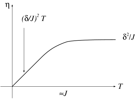
FIG. 6.: Simplest scenario of the temperature dependence of the linewidth in the presence of an exchange anisotropy. The $T$-linear behavior at low temperature predicted by the field theory method crossovers smoothly to the constant $\sim\delta^{2}/J$ predicted by the Kubo-Tomita theory at high temperature limit. The crossover takes place at $T\sim J$, which is the limit of the validity of the field theory approach.

For the exchange anisotropy (59) in a generic direction, the KT formula (12) has been applied to the linewidth in the literature. The result is

$$\eta\propto\frac{\delta^{2}}{J},$$ (188)

where we have ignored the direction dependence. It is difficult to discuss the intermediate temperature regime either with the existing theories or with our field theory approach. However, our result can be naturally related to the high-temperature limit, assuming a smooth crossover at temperature $T\sim J$, namely if the $T$-linear behavior (68),(136) is cut off at $T\sim J$ as shown in Fig. 6. In fact, this simple scenario seems to agree with the experimental results[35, 36, 37, 34, 39, 40] on CPC, KCuF₃, CuGeO₃ and NaV₂O₅, which we think the exchange anisotropy (including the dipolar interaction) is the primary mechanism of the broadening. See Fig. 4 for some of the examples.

We note that, while the low-temperature asymptotic behavior described by the field theory is universal, the crossover to the high-temperature regime is expected to be non-universal. The linewidth as a function of the temperature would depend, for example, on the next-nearest-neighbor interaction introduced additionally to the standard Hamiltonian (22).

B Staggered field

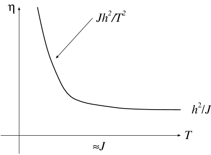
FIG. 7.: Simplest scenario of the temperature dependence of the linewidth in the presence of a staggered field, interpolating the low-temperature field theory result $Jh^{2}/T^{2}$ and the high-temperature result $h^{2}/J$.

No literature on the effect of a staggered field in ESR linewidth is known to us. The application of the KT formula (12) to the staggered field perturbation (158) is nevertheless straightforward, giving the linewidth

$$\eta\propto\frac{h^{2}}{J},$$ (189)

at the high temperature limit. This is again consistent with the low-temperature field theory result eq. (166), assuming a smooth crossover at $T\sim J$, as shown in Fig. 7.

C Dzyaloshinskii-Moriya interaction

While the effects of a DM interaction (57) has been discussed in the literature[33, 34, 38], we believe there is a rather serious problem with these previous treatments. A direct application of the KT formula (12), as was made previously, yields the width

$$\eta\propto\frac{D^{2}}{J},$$ (190)

where we have again ignored the angle dependence.

On the other hand, a staggered DM interaction can be reduced to an exchange interaction $\delta\sim D^{2}/J$ and a transverse staggered field $h\sim DH/J$ via an exact transformation discussed in Sec. III B 1. If we apply the KT formula after the transformation, we obtain

$$\eta\propto\frac{D^{4}}{J^{3}}+\frac{D^{2}H^{2}}{J^{3}},$$ (191)

where we ignored constants of $O(1)$. This actually differs substantially from the result of the direct application (190). In a typical situation, $D/J\sim 0.1$ and $H\ll D<J$ so that $\eta\sim 0.01J$ from eq. (190) while $\eta\sim 10^{-4}J$ from eq. (191), which means a factor of $100$ difference. (Actually we have to know the numerical coefficient, which has been ignored so far, in order to discuss the absolute value of the width.) In addition, it is argued[28] that there exists an exchange anisotropy (before the transformation) which accompanies the DM interaction, and cancels the anisotropy coming from the DM interaction. The discrepancy would be even greater when this happens.

Obviously, both results cannot be true at the same time (while they could be both wrong.) What we believe is that the latter approach eliminating the DM interaction first is appropriate, and the direct application of the KT formula to the DM interaction is incorrect. A possible reason why the direct application (190) fails is as follows. In the latter approach based on the transformation (191), the physical total spin operator $S^{x,y}$ is actually given by a sum of the total spin operator and the staggered spin operator of the model after the transformation. Thus, the physical absorption spectrum of ESR is also given by the sum of contributions from the uniform and staggered part:

$$\chi^{\prime\prime}_{\rm phys}(q=0,\omega)\sim\chi^{\prime\prime}(q=0,\omega)+\left(\frac{D}{J}\right)^{2}\chi^{\prime\prime}(q=\pi,\omega),$$ (192)

where $\chi^{\prime\prime}$ is the imaginary part of the dynamical susceptibility for the transformed model. The staggered part $\chi^{\prime\prime}(q=\pi,\omega)$ is already broad even in the absence of the anisotropic perturbation, and is further suppressed by the factor $(D/J)^{2}$. Thus it would be practically indistinguishable from the background, especially in the high temperature regime. The main absorption due to the $\chi^{\prime\prime}(q=0,\omega)$ term is presumably Lorentzian with the width given by (191). According to this picture, the lineshape is not a single Lorentzian, although apparently it is. The direct application of the KT formula misses such a structure, and treats all the effects as if the lineshape is a single Lorentzian. This presumably leads to the incorrect result (190).

An indirect evidence of our claim is that the elimination seems to work well in the field theory of ESR at low temperature. Assuming a smooth crossover at $T\sim J$, the latter result (191) seems more plausible. In addition, a recent experiment[9] on a very good one-dimensional $S=1/2$ Heisenberg antiferromagnet Pyrimidine Cu dinitrate strongly suggests that there is a staggered DM interaction along the chain, resulting in the field-induced gap similar to that observed in Cu benzoate. An analysis of various experimental data suggests[9] that the staggered DM interaction $D\sim 0.14J$, where the exchange coupling in this compound is $J\sim 36{\rm K}$. According to the direct approach (190), the linewidth at high temperature should be of the order of $D^{2}/J\sim 5000{\rm Oe}$. This might be too large to understand the observed small linewidth $\sim 20{\rm Oe}$ at room temperature[9], which is quite high compared to the exchange interaction $J$. On the other hand, if we use eq. (191) and $H\ll D$, the estimate of the linewidth becomes to be of order of $D^{4}/J^{3}\sim 100{\rm Oe}$, which is not too far from the experimental result. We note that we do not know the numerical coefficients and thus a conclusive quantitative discussion is difficult. In addition, the exchange anisotropy (before the elimination of the DM interaction), which is ignored in the above estimate, is not known precisely. Nevertheless, considering the significant difference, the observed linewidth in pyrimidine Cu dinitrate could serve as an experimental support for our claim that the direct treatment of the DM interaction is inappropriate.

On the other hand, we do not understand at present how to deal with a uniform DM interaction along the chain. While it can be eliminated by a similar transformation as well, the result contains the magnetic field rotating in its direction along the chain. This is a rather unfamiliar problem which we do not know how to handle at present.

D High-temperature expansion of the linewidth

In a series of papers, Yamada and collaborators studied the temperature dependence of ESR linewidth in one dimensional magnetic systems experimentally and theoretically. In the theoretical study, they discussed the temperature dependence by a high-temperature expansion of the KT formula. More precisely, they attempted a high-temperature expansion of $\langle{\cal A}{\cal A}^{\dagger}\rangle$ in the numerator of the KT formula, Eq. (12).

They concluded that for an exchange anisotropy the linewidth increases as the temperature is lowered, while the tendency is the opposite for a (uniform or staggered) DM interaction. Based on this observation, they argued that the DM interaction should be dominant in several one-dimensional antiferromagnets which showed a decreasing linewidth at lower temperature. In some cases the DM interaction is forbidden according to the previously identified crystal symmetry; they went on to the conclusion that the actual symmetry is lower than what had been believed, allowing the DM interaction.

However, their argument is to be criticized on several grounds. First, the high-temperature expansion can not be trusted except for very high temperature. At $T\ll J$ our field theory approach should be more reliable, and it gives a rather opposite result to their claim. Second, they expand only the numerator $\langle{\cal A}{\cal A}^{\dagger}\rangle$ in the KT formula to the first order in $1/T$, ignoring other possible contributions of order $1/T$. It is not clear to us whether their scheme makes sense as a $1/T$ expansion of the linewidth. Third, perhaps most importantly, even in their framework of the calculation, the conclusion should be reversed because they apparently made a crucial sign mistake as we will show below. Finally, they apply the KT formula directly to the DM interaction; this is problematic as we have pointed out. In any case, the sign problem persists whether the direct approach or the elimination approach is taken in dealing with the DM term.

In the following, let us show that the sign should be reversed within the framework of Refs. [34, 38, 39, 40]. We consider $S=1/2$ Heisenberg antiferromagnetic chains with a small perturbation. First let us discuss the case of an anisotropy parallel to the applied field. The calculation for general anisotropy angle should be similar. This gives the commutator

$${\cal A}=[{\cal H}^{\prime},S^{+}]=\delta\sum_{j}(S^{+}_{j}S^{z}_{j+1}+S^{z}_{j}S^{+}_{j+1}).$$ (193)

The “numerator” of the KT formula is then given by

$$\langle{\cal A}{\cal A}^{\dagger}\rangle=\delta^{2}\sum_{j,k}\langle(S^{+}_{j}S^{z}_{j+1}+S^{z}_{j}S^{+}_{j+1})(S^{-}_{k}S^{z}_{k+1}+S^{z}_{k}S^{-}_{k+1})\rangle.$$ (194)

Considering the high-temperature limit we can ignore all but nearest-neighbor correlations. Thus we only consider the $j=k$ terms in the double sum;

$$\langle[{\cal H}^{\prime},S^{+}][S^{-},{\cal H}^{\prime}]\rangle\sim\delta^{2}N[\frac{1}{4}+\frac{\langle S^{z}\rangle}{2}+\langle S^{x}_{j}S^{x}_{j+1}\rangle],$$ (195)

where we have used identities for $S=1/2$, such as $S^{+}_{j}S^{-}_{j}=S^{z}_{j}+1/2$ and $N$ is the number of sites. In the limit of infinite temperature, the width is given by the first term which is $\delta^{2}/J$ as was already discussed.

As the temperature is lowered from infinity, the leading correction is given by the second and third terms. The second term proportional to the magnetization $\langle S^{z}\rangle$ is negligible compared to the third term in our case $H\ll J$. The third term represents the nearest-neighbor correlation effect, and should be proportional to $-J/T$ at high temperature $T$. Note that we are dealing with an antiferromagnet, so that the nearest-neighbor correlation should be negative. Ignoring other possible sources of temperature dependence following Refs. [34, 38, 39, 40], the linewidth in the present case is given by

$$\eta=\frac{{\delta}^{2}}{J}[a-b\frac{J}{T}+O(\frac{J^{2}}{T^{2}})],$$ (196)

with positive coefficients $a,b$ for an antiferromagnet. Namely, the linewidth decreases at lower temperature contrary to the claims made in Refs. [34, 38, 39, 40]; this is rather natural from the field theory results at low temperatures as discussed in Section IX A. It appears that, they took the nearest-neighbor correlation as positive, which is valid for a ferromagnet[52] but not for an antiferromagnet.

Now let us consider the transverse staggered field perturbation in the same framework. In this case, ${\cal A}=[{\cal H}^{\prime},S^{+}]=-h\sum_{j}(-1)^{j}S^{z}_{j}$, which gives the “numerator”

$$\langle{\cal A}{\cal A}^{\dagger}\rangle=h^{2}\sum_{j,k}(-1)^{j+k}\langle S^{z}_{j}S^{z}_{k}\rangle.$$ (197)

In the high-temperature limit, we may ignore all the correlation functions other than the nearest neighbor one. This leads to the formula

$$\langle{\cal A}{\cal A}^{\dagger}\rangle=h^{2}N[\frac{1}{4}-2\langle S^{z}_{j}S^{z}_{j+1}\rangle]$$ (198)

Considering that the nearest-neighbor correlation is negative for an antiferromagnet, the linewidth is supposed to be given as

$$\eta=\frac{h^{2}}{J}[a^{\prime}+b^{\prime}\frac{J}{T}+O(\frac{J^{2}}{T^{2}})],$$ (199)

where $a^{\prime}$ and $b^{\prime}$ are positive constants. Namely, the linewidth increases at lower temperature; again in a qualitative agreement with the field theory.

For a staggered DM interaction, as we have discussed before, presumably we should first eliminate the DM interaction to reduce the problem to the exchange anisotropy and the transverse staggered field. In a typical situation $H\ll D\ll J$, the staggered field $h\sim DH/J$ and the anisotropy $\delta\sim D^{2}/J$ induced by the transformation satisfy $h\ll\delta\ll J$. In this case, the linewidth would initially decrease by lowering the temperature, then start increasing below the crossover temperature where the staggered field becomes dominant. This was actually observed in Cu benzoate, as discussed already in Section VIII D.

Finally, we consider a direct application of the KT formula to the DM interaction. Although we believe this is not an adequate approach, the claims in Refs. [34, 38, 39, 40] still suffers from the same sign problem even if we accept the direct approach. Now we have

$${\cal A}=[{\cal H}^{\prime},S^{+}]=\sum_{j}D_{j}i(S^{z}_{j}S^{+}_{j+1}-S^{+}_{j}S^{z}_{j+1}),$$ (200)

giving

$$\langle{\cal A}{\cal A}^{\dagger}\rangle\sim D^{2}N[1-\langle S^{x}_{j}S^{x}_{j+1}\rangle],$$ (201)

ignoring other than next-nearest-neighbor correlation in the high-temperature limit. Because the nearest neighbor correlation function is negative in an antiferromagnet, we obtain

$$\eta=\frac{D^{2}}{J}[a^{\prime\prime}+b^{\prime\prime}\frac{J}{T}+O(\frac{J^{2}}{T^{2}})],$$ (202)

where $a^{\prime\prime}$ and $b^{\prime\prime}$ are positive constants, implying the increasing linewidth at lower temperatures. The error in Refs. [34, 38, 39, 40] is again apparently due to the identification of the nearest-neighbor correlation as positive.

X Conclusions

In this paper, we have developed a new approach based on field theory to ESR in quantum spin chains. It is expected to be exact in the low-energy (low-temperature) limit, precisely where the traditional calculational methods on ESR become invalid. The weakly broken $SU(2)$ symmetry under an applied field, in the absence of an anisotropic perturbation, is represented by the $SU(2)$ symmetric field theory and an anisotropic mapping between the physical spin operators and the corresponding field theory operators.

The formulation of the ESR in terms of Feynman-Dyson self-energy gives, at least in some simple cases, a microscopic derivation of the Lorentzian lineshape up to a possible smooth weak background. The spin diffusion picture[4], which predicts a non-Lorentzian lineshape in one dimension, does not apply to the $S=1/2$ antiferromagnetic chain at low temperature. The spin diffusion hypothesis does not hold in the present case, as the spin correlation function is given explicitly using eq. (42).

The width and shift are calculated perturbatively for a transverse staggered field perturbation and an exchange anisotropy parallel or perpendicular to the applied uniform field. They seem to explain many existing experimental data. Furthermore, the self-energy formulation can be used beyond the perturbation theory. In fact, in the presence of a staggered field, the perturbation theory breaks down at a low enough temperature. The ESR spectrum in the zero temperature limit is discussed with a non-perturbative treatment of the sine-Gordon field theory. This again seem to explain the experimentally observed ESR lineshape in Cu benzoate at very low temperature.

While our field theory approach works only at low temperatures, we have also discussed a few aspects of ESR at higher temperatures. In particular, we have pointed out that a naive application of the standard Kubo-Tomita theory fails even in the high temperature limit, in the presence of a Dzyaloshinskii-Moriya interaction.

We hope that the reader is convinced that ESR in a strongly interacting quantum system is quite an interesting problem from the theoretical point of view. It is also a useful experimental probe because a very precise spectrum can be obtained.

Obviously, there remain many problems to be investigated in the future. Even in the simple quantum antiferromagnetic chain, the formulation of ESR in terms of self-energy of the boson field $\phi$ does not hold for generic types of anisotropic perturbations, because of the mixing of several operators. Extension of the self-energy formulation to the generic cases is an important open problem; presumably we have to consider perturbative expansion of correlation functions of the vertex operators (exponentials of the boson field) in a systematic way. Moreover, degrees of freedom other than spins (e.g. charge fluctuation, lattice vibration etc.) will be relevant in some real materials. While the ESR in a three-dimensional magnet appears to be understood with the existing theory[2, 3], we think that the problem should be reinvestigated with the modern understanding of many-body physics and critical phenomena. Naturally, the two-dimensional problem, which is expected to be more sensitive to the fluctuation effects, would also deserve consideration. We hope the present work will stimulate further theoretical and experimental studies on this fascinating subject.

Note Added. After submitting the present paper, a paper by Choukroun, Richard and Stepanov was published[53]. They made a similar proposal to ours (Sec. IX C in the present paper) on the treatment of the Dzyaloshinskii–Moriya interaction at high temperature limit.

A Alternative derivation of the Mori-Kawasaki formula

In this appendix, we describe a simple alternative derivation of the MK formula (7),(10) suggested to us by David M. Edwards. It depends only on the assumption that the lineshape takes a single Lorentzian form, and appears much simpler than that in the original paper[2]. On the other hand, it does not answer the question why (and when) the lineshape takes the Lorentzian form.

We consider ESR in a general spin system given by the Hamiltonian (6). Here and in the following, a spin operator without a site index is regarded as the total spin operator $S^{\alpha}=\sum_{j}S^{\alpha}_{j}$. The equations of motion for $S^{\pm}$ are given by

$$\frac{dS^{+}}{dt} = -iHS^{+}+i{\cal A}$$ (A1)

$$\frac{dS^{-}}{dt} = +iHS^{-}-i{\cal A}^{\dagger},$$ (A2)

where ${\cal A}=[{\cal H}^{\prime},S^{+}]$.

The ESR spectrum can be obtained from the Green’s function of $S^{\pm}$. Let us relate this to the Green’s function of ${\cal A}$ and ${\cal A}^{\dagger}$, using the equations of motion. Using a partial integration and the equations of motion,

$${\cal G}^{R}_{S^{+}S^{-}}(\omega) = -i\int_{0}^{\infty}e^{i\omega t}\langle[S^{+}(t),S^{-}(0)]\rangle dt$$ (A3)

$$= \frac{1}{\omega}\langle[S^{+}(0),S^{-}(0)]\rangle+\frac{1}{\omega}\int_{0}^{\infty}e^{i\omega t}\langle[\frac{dS^{+}}{dt}(t),S^{-}(0)]\rangle dt$$ (A4)

$$= \frac{2\langle S^{z}\rangle}{\omega}+\frac{H}{\omega}{\cal G}^{R}_{S^{+}S^{-}}(\omega)-\frac{1}{\omega}{\cal G}^{R}_{{\cal A}S^{-}}(\omega).$$ (A5)

Thus

$${\cal G}^{R}_{S^{+}S^{-}}(\omega)=\frac{2\langle S^{z}\rangle-{\cal G}^{R}_{{\cal A}S^{-}}}{\omega-H}.$$ (A6)

(Precisely speaking we should introduce the convergence factor so that $\omega-H$ is replaced by $\omega-H+i\epsilon$ with a positive infinitesimal $\epsilon$. Although we omit this for brevity, it can be recovered when necessary.) Performing similar steps,

$${\cal G}^{R}_{{\cal A}S^{-}}(\omega) = -i\int_{0}^{\infty}e^{i\omega t}\langle[{\cal A}(t),S^{-}(0)]\rangle dt$$ (A7)

$$= \frac{1}{\omega}\langle[{\cal A}(0),S^{-}(0)]\rangle-\frac{1}{\omega}\int_{0}^{\infty}e^{i\omega t}\langle[{\cal A}(t),\frac{dS^{-}}{dt}(0)]\rangle dt$$ (A8)

$$= +\frac{\langle[{\cal A}(0),S^{-}(0)]\rangle}{\omega}+\frac{H}{\omega}{\cal G}^{R}_{{\cal A}S^{-}}(\omega)-\frac{1}{\omega}{\cal G}^{R}_{{\cal A}{\cal A}^{\dagger}}(\omega),$$ (A9)

where we used the relation

$$\frac{d}{dt}\langle[{\cal A}(t),S^{-}(0)]\rangle=-\langle[{\cal A}(t),\frac{dS^{-}}{dt}(0)]\rangle$$ (A10)

which holds because the Green’s function depends only on the difference of two time arguments. Thus

$${\cal G}^{R}_{{\cal A}S^{-}}(\omega)=\frac{\langle[{\cal A}(0),S^{-}(0)]\rangle-{\cal G}^{R}_{{\cal A}{\cal A}^{\dagger}}(\omega)}{\omega-H}.$$ (A11)

Combining eqs. (A6) and (A11), we obtain

$${\cal G}^{R}_{S^{+}S^{-}}(\omega)=\frac{2\langle S^{z}\rangle}{\omega-H}+\frac{-\langle[{\cal A}(0),S^{-}(0)]\rangle+{\cal G}^{R}_{{\cal A}{\cal A}^{\dagger}}(\omega)}{(\omega-H)^{2}}.$$ (A12)

This should be an exact relation between the full Green’s functions (in which the effect of the perturbation ${\cal H}^{\prime}$ is fully taken into account.) When ${\cal H}^{\prime}=0$, we recover the simple result ${\cal G}^{R}_{S^{+}S^{-}}(\omega)=2\langle S^{z}\rangle/(\omega-H)$.

Now let us assume the perturbation ${\cal H}^{\prime}$ is small, and the ESR lineshape is Lorentzian. Namely, we assume that ${\cal G}^{R}_{S^{+}S^{-}}(\omega)$ is given by eq. (11) where $\Sigma$ is a smooth function of $\omega$. Near the resonance $\omega\sim H$, $\Sigma$ may be regarded as a constant. ${\rm Re}\Sigma$ and $-{\rm Im}\Sigma$ gives the shift and width of the resonance, respectively. We assume that $\Sigma$ can be expanded perturbatively in ${\cal H}^{\prime}$.

Comparing eqs. (11) and (A12), we obtain, in the lowest order of perturbation theory,

$$\Sigma\sim\frac{-\langle[{\cal A}(0),S^{-}(0)]\rangle+{\cal G}^{R}_{{\cal A}{\cal A}^{\dagger}}(\omega=H)}{2\langle S^{z}\rangle}.$$ (A13)

Here we note that $\langle[{\cal A}(0),S^{-}(0)]\rangle$ is purely real since $[{\cal A},S^{-}]$ is Hermitean. This gives

$$\eta = \frac{-1}{2\langle S^{z}\rangle}{\rm Im}{\cal G}^{R}_{{\cal A}{\cal A}^{\dagger}}(\omega=H),$$ (A14)

$$\Delta\omega = \frac{1}{2\langle S^{z}\rangle}\left[-\langle[{\cal A},S^{-}]\rangle+{\rm Re}{\cal G}^{R}_{{\cal A}{\cal A}^{\dagger}}(\omega=H)\right].$$ (A15)

For a small field $H$, the denominator $2\langle S^{z}\rangle$ can be written as $2\chi_{u}H$ where $\chi_{u}$ is the uniform susceptibility. We also note that the first term in the shift $-\langle[{\cal A},S^{-}]\rangle/(2\langle S^{z}\rangle)$ was derived previously by Kanamori and Tachiki[47], and by Nagata and Tazuke[48]. However, their theory did not incorporate the dynamical effects represented by ${\cal G}^{R}_{{\cal A}{\cal A}^{\dagger}}$.

So far, we have defined the expectation value and the Green’s functions with respect to the full Hamiltonian ${\cal H}={\cal H}_{0}+{\cal H}_{Z}+{\cal H}^{\prime}$. However, the present result is only valid in the leading order. Since the Green’s function of ${\cal A}$ above already contains the factor $\lambda^{2}$ ($\lambda$ is the small parameter that characterizes the perturbation ${\cal H}^{\prime}$), we may replace ${\cal G}^{R}_{{\cal A}{\cal A}^{\dagger}}$ with the unperturbed Green’s function $G^{R}_{{\cal A}{\cal A}^{\dagger}}$. This gives the formulae in eqs. (7) and (10). We note that, in general, $\langle[{\cal A},S^{-}]\rangle$ must still be evaluated in the presence of ${\cal H}^{\prime}$ because $[{\cal A},S^{-}]$ is only first order in $\lambda$.

REFERENCES

- [1] R. Kubo and K. Tomita, J. Phys. Soc. Jpn. 9, 888 (1954).
- [2] H. Mori and K. Kawasaki, Prog. Theor. Phys. 27, 529 (1962).
- [3] H. Mori and K. Kawasaki, Prog. Theor. Phys. 28, 971 (1962).
- [4] R. E. Dietz, F. R. Merritt, R. Dingle, D. Hone, B. G. Silbernagel and P. M. Richards, Phys. Rev. Lett. 26, 1186 (1971).
- [5] D.C. Dender, P.R. Hammar, D.H. Reich, C. Broholm and G. Aeppli, Phys. Rev. Lett. 79, 1750 (1997).
- [6] M. Oshikawa and I. Affleck, Phys. Rev. Lett. 79, 2883 (1997).
- [7] I. Affleck and M. Oshikawa, Phys. Rev. B 60, 1038 (1999).
- [8] M. Oshikawa, K. Ueda, H. Aoki, A. Ochiai and M. Kohgi, J. Phys. Soc. Jpn. 68, 3181 (1999).
- [9] R. Feyerherm, S. Abens, D. Günther, T. Ishida, M. Meissner, M. Meschke, T. Nogami and M. Steiner, J. Phys.: Condens. Matter 12, 8495 (2000).
- [10] K. Okuda, H. Hata and M. Date, J. Phys. Soc. Jpn. 33, 1574 (1972)
- [11] K. Oshima, K. Okuda and M. Date, J. Phys. Soc. Jpn. 44, 757 (1978).
- [12] M. Oshikawa and I. Affleck, Phys. Rev. Lett. 82, 5136 (1999).
- [13] S. C. Zhang, Science 275, 1089 (1997).
- [14] S. Miyashita, T. Yoshino and A. Ogasahara, J. Phys. Soc. Jpn. 68, 655 (1999).
- [15] Y. Natsume, F. Sasagawa, M. Toyoda and I. Yamada, J. Phys. Soc. Jpn. 48, 50 (1980).
- [16] I. Yamada and Y. Natsume, J. Phys. Soc. Jpn. 48, 58 (1980).
- [17] Y. Natsume, F. Noda, F. Sasagawa and H. Kanazawa, J. Phys. Soc. Jpn. 52, 1427 (1983).
- [18] I. Affleck, in Fields, Strings and Critical Phenomena, Les Houches, Session XLIX, ed. by E. Brézin and J. Zinn-Justin, North-Holland, Amsterdam (1988).
- [19] A. O. Gogolin, A. A. Nersesyan and A. M. Tsvelik, Bosonization and Strongly Correlated Systems, Cambridge University Press (1998).
- [20] N. Ishimura and H. Shiba, Prog. Theor. Phys. 63, 743 (1980).
- [21] G. Müller, H. Thomas, H. Beck, and J. C. Bonner, Phys. Rev. B 24, 1429 (1981).
- [22] M. Yamanaka, M. Oshikawa and I. Affleck, Phys. Rev. Lett. 79, 1110 (1997).
- [23] V. E. Korepin, N. M. Bogoliubov and A. G. Izergin, Quantum Inverse Scattering Method and Correlation Functions, Cambridge University Press (1993).
- [24] H. J. Schulz, Phys. Rev. B 34, 6372 (1986).
- [25] I. Affleck, D. Gepner, H. J. Schulz, and T. Ziman, J. Phys. A 22, 511 (1989).
- [26] I. Dzyaloshinskii, J. Phys. Chem. Solids 4, 241 (1958).
- [27] T. Moriya, Phys. Rev. 120, 91 (1960).
- [28] T. A. Kaplan, Z. Phys. B 49, 313 (1983); L. Shekhtman, O. Entin-Wohlman and A. Aharony, Phys. Rev. Lett. 69, 836 (1992).
- [29] S. Eggert, I. Affleck and M. Takahashi, Phys. Rev. Lett. 73, 332 (1994).
- [30] T. Giamarchi, Phys. Rev. B 44, 2905 (1991); Phys. Rev. B 46, 342 (1992).
- [31] T. Giamarchi and A.J. Millis, Phys. Rev. B 46, 9325 (1992).
- [32] W. Götze and P. Wölfle, Phys. Rev. B 6, 1226 (1972);
- [33] M. Date, H. Yamazaki, M. Motokawa and S. Tazawa, Suppl. Prog. Theor. Phys. 46, 194 (1970).
- [34] I. Yamada, H. Fujii and M. Hidaka, J. Phys. Condens. Matter 1, 3397 (1989);
- [35] Y. Ajiro, S. Matsukawa, T. Yamada and T. Haseda, J. Phys. Soc. Jpn. 39, 259 (1975).
- [36] H. Ohta, S. Imagawa, H. Ushiroyama, M. Motokawa, O. Fujita and J. Akimitsu, J. Phys. Soc. Jpn. 65, 691 (1996).
- [37] S. V. Demishev, A. V. Semeno, N. E. Sluchanko, N. A. Samarin, A. N. Vasil’ev and L. I. Leonyuk, JETP 85, 943 (1997).
- [38] T. Ishii and I. Yamada, J. Phys. Condens. Matter 2, 7339 (1990);
- [39] I. Yamada, M. Nishi and J. Akimitsu, J. Phys. Condens. Matter 8, 2625 (1996);
- [40] I. Yamada, H. Manaka, H. Sawa, M. Nishi, M. Isobe and Y. Ueda, J. Phys. Soc. Jpn. 67, 4269 (1998).
- [41] A. A. Zvyagin, Phys. Rev. B 63, 172409 (2001).
- [42] I. Affleck, J. Phys. A31, 4573 (1998).
- [43] S. Lukyanov and A. Zamalodchikov, Nucl. Phys. B493, 571 (1997).
- [44] S. Lukyanov, preprint cond-mat/9712314.
- [45] T. Asano, H. Nojiri, Y. Inagaki, J. P. Boucher, T. Sakon, Y. Ajiro and M. Motokawa, Phys. Rev. Lett. 84, 5880 (2000).
- [46] K. Nagata, J. Phys. Soc. Jpn. 40, 1209 (1976).
- [47] J. Kanamori and M. Tachiki, J. Phys. Soc. Jpn. 17, 1384 (1962).
- [48] K. Nagata and Y. Tazuke, J. Phys. Soc. Jpn. 32, 337 (1972).
- [49] K. Oshima, K. Okuda and M. Date, J. Phys. Soc. Jpn. 41, 475 (1976).
- [50] M. Karowski and P. Weisz, Nucl. Phys. B139, 445 (1978).
- [51] H. Nojiri, private communications (2000).
- [52] Z. G. Soos, K. T. McGregor, T. T. P. Cheung and A. J. Silverstein, Phys. Rev. B 16, 3036 (1977).
- [53] J. Choukroun, J.-L. Richard and A. Stepanov, Phys. Rev. Lett. 87, 127207 (2001).