Phase transitions at surfaces, edges, and corners

Abstract

Results of large-scale Monte Carlo simulations of three-dimensional Ising models with edges and corners are reviewed. At the ordinary transition, angle dependent critical exponents are observed, whereas at the surface transition edge and corner critical exponents are non-universal and depend on the details of the model. The results obtained at the surface transition are compared to exact findings on critical two-dimensional Ising models with different types of defect lines.

1 Introduction

Critical phenomena at perfect, flat surfaces of three-dimensional systems have been the subject of intensive research during the last three decades [1, 2, 3]. For the three-dimensional semi-infinite Ising model two different ferromagnetic couplings are usually introduced, depending on whether the neighbouring spins are both located at the surface, $J_{s}>0$, or not, $J_{b}>0$. The resulting phase diagram is well established. If the ratio of the surface coupling $J_{s}$ to the bulk coupling $J_{b}$, $r=J_{s}/J_{b}$, is sufficiently small, the system undergoes at the bulk critical temperature $T_{c}$ an ordinary transition, with the bulk and surface ordering occurring at the same temperature. Beyond a critical ratio, $r>r_{sp}\approx 1.50$ [4, 5], the surface orders at a higher temperature $T_{s}>T_{c}$ at the surface transition, followed by the extraordinary transition of the bulk at $T_{c}$. At the critical ratio $r_{sp}$, one encounters the multicritical special transition point.

The semi-infinite Ising model with a flat surface may be considered to be a special case of a more complex wedge geometry where two planes meeting at an angle $\theta$ form an infinite edge. For $\theta=\pi$ the flat surface is recovered. Cardy [6] showed that at the ordinary transition edge critical exponents depending continuously on $\theta$ arise on purely geometrical grounds. For a given opening angle $\theta$, however, the values of the critical exponents are expected to be universal and independent on microscopic details like the strengths of the coupling constants or the lattice type. Whereas edge singularities at the ordinary transition have been studied intensively, especially in two dimensions [7], edge critical behaviour at the surface transition of three-dimensional Ising models has been largely overlooked. At the surface transition the critical fluctuations are essentially of two-dimensional character. One may then argue that the edge should act like a local perturbation in a two-dimensional system. In analogy with exact results obtained for two-dimensional Ising models with defect lines [8], intriguing nonuniversal edge critical behaviour is therefore expected. Similarly, corner critical exponents depending on the details of the model should also be observed at the surface transition.

In this contribution, I discuss results on edge and corner critical behaviour obtained in large-scale Monte Carlo simulations of three-dimensional Ising models [9, 10, 11]. After presenting some details of the simulations in the next Section, I then discuss edge and corner criticality at the ordinary (Section 3) and at the surface transition (Section 4). A brief summary concludes the paper.

2 Models with edges and corners

To introduce edges in Ising magnets defined on simple cubic lattices, periodic boundary conditions along one axis, the $z$-axis, are applied. The remaining four free surfaces of the crystal may be oriented in various ways leading to different opening angles $\theta$ at the edges. As shown in Figure 1, pairs of (100) and (010) surfaces lead to four equivalent edges with opening angles $\theta=\pi/2$. The intersection of (100) and (110) surfaces form two pairs of edges with $\theta=\pi/4$ and $\theta=3\pi/4$, see Figure 2. Besides the bulk coupling $J_{b}$ and the surface coupling $J_{s}$, further couplings may be introduced [9, 10]: two neighbouring edge spins interact with the edge coupling $J_{e}$, whereas an edge spin is coupled to its neighbouring surface spin by the edge-surface interaction $J_{es}$. The Hamiltonian is then given by

$$H = -\sum\limits_{bulk}J_{b}S_{{\bf r}}S_{{\bf r}^{\prime}}-\sum\limits_{surface}J_{s}S_{{\bf r}}S_{{\bf r}^{\prime}}$$ (1)

$$-\sum\limits_{edge-surface}J_{es}S_{{\bf r}}S_{{\bf r}^{\prime}}-\sum\limits_{edge}J_{e}S_{{\bf r}}S_{{\bf r}^{\prime}}$$

with spins $S_{{\bf r}}=\pm 1$ at sites ${\bf r}=(xyz)$. For the study of corners we use free boundary conditions in all three directions. The couplings between corner spins and neighbouring edge spins are set equal to $J_{e}$, thus regarding corners as endpoints of edges.

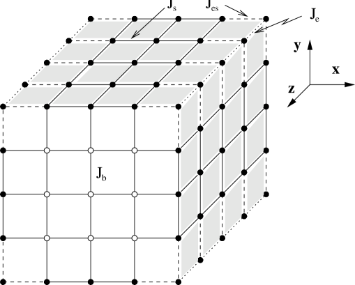
Figure 1: Geometry of an Ising model with (100) and (010) surfaces forming edges with opening angles $\theta=\pi/2$.

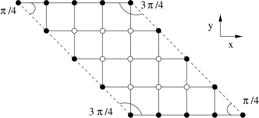
Figure 2: Geometry of a model with edges with opening angles $\theta=\pi/4$ and $\theta=3\pi/4$. Shown is a cut through the crystal perpendicular to the edge direction. The full lines represent the couplings between neighbouring spins, whereas the (110) surfaces are indicated by the dashed lines.

The results presented in the following have been obtained with the efficient one-cluster-flip algorithm [12]. Systems with $L\times L\times N$ sites were considered, with $L\times L$ being the number of sites in the planes perpendicular to the $z$-axis, and $N$ being the number of sites along that axis. $L$ ranged from 10 to 80 and $N$ from 10 to 640. For the investigation of corner critical behaviour Ising cubes with up to $80^{3}$ spins were simulated.

As we aim at studying properties of systems with infinitely long edges, finite-size effects have to be monitored closely. The Monte Carlo system should be large enough to reproduce the thermodynamic values of the bulk and the surface magnetization sufficiently far away from the edge. In general, at a given temperature, edge quantities must be stable against enlargening the system size. The same holds for corner quantities.

An interesting quantity in systems without corners is the magnetization per site for lines parallel to the $z$-axis:

$$m(x,y)=\langle|\sum\limits_{z}S_{xyz}|\rangle/N.$$ (2)

The sum runs over the $N$ spins in a line, with $x$ and $y$ being fixed. The brackets denote thermal averages. As usual, the absolute value is taken to avoid vanishing magnetizations for finite systems.

From the line magnetizations, various magnetizations of interest are obtained. The edge magnetization $m_{2}$ is identical to

$$m_{2}=\langle|\sum\limits_{z}S_{x_{0}y_{0}z}|\rangle/N$$ (3)

where $(x_{0}y_{0}z)$ denotes an edge site. The surface magnetization results from the line magnetization in the center of a surface, whereas the bulk magnetization is given by the line magnetization in the middle of the crystal.

The local magnetization $m_{l}(x,y,z)$ may be obtained by computing the correlation function $\left<S_{xyz}\,S_{x^{\prime}y^{\prime}z^{\prime}}\right>$ between topologically equivalent sites ($xyz$) and ($x^{\prime}y^{\prime}z^{\prime}$) with maximal separation distance. In this way, the corner magnetization of Ising cubes with linear dimension $L$ is given by

$$m_{3}=\sqrt{\langle S_{000}\,S_{LLL}\rangle}.$$ (4)

I refer to corner quantities by the subscript 3 (indicating that three planes meet at this point), whereas edge quantities have the subscript 2.

3 Ordinary transition

In [6], Cardy considered $d$-dimensional systems with $(d-1)$-dimensional hyperplanes meeting at an angle $\theta$. At the bulk critical point local critical exponents changing continuously with $\theta$ are already obtained in mean-field approximation. Cardy showed that all edge critical exponents can be obtained by combining bulk and surface critical exponents with a new angle dependent edge exponent. He also computed the value of this exponent in first order of an $\epsilon=d-4$ expansion. From the renormalization group point of view, the angle dependence has its origin in the invariance of the edge under rescaling. This makes the opening angle to a marginal variable, which may then lead to angle dependent local critical exponents.

Edge magnetizations computed by Monte Carlo simulations are plotted in Figure 3 for four different opening angles: $\theta=\pi/4$, $\pi/2$, $3\pi/4$, and $\pi$ (correponding to the free surface), with all coupling constants set equal to $J_{b}$. Only data presenting no noticeable finite-size dependences are displayed. This is achieved by studying systems with a large number of edge sites, the edge length being the crucial quantity [9].

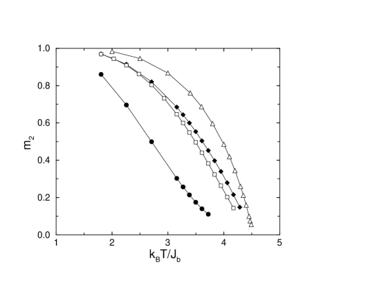
Figure 3: Edge magnetization versus temperature for various opening angles $\theta$: $\pi/4$ (circles), $\pi/2$ (squares), $3\pi/4$ (diamonds), and $\pi$ (triangles). Only data not affected by finite-size effects are displayed. Error bars are smaller than the size of the symbols.

At the ordinary transition, the edge magnetizations vanish at the bulk critical temperature $k_{B}\,T_{c}/J_{b}\approx 4.5115$ with a power law behaviour $m_{2}\sim(T_{c}-T)^{\beta_{2}}$. Here, $\beta_{2}$ is the critical exponent of the edge magnetization. In order to estimate $\beta_{2}$, one may study [13] an effective temperature dependent exponent $\beta_{2,eff}(t)$ defined by

$$\beta_{2,eff}(t)=\mbox{d}\ln m_{2}/\mbox{d}\ln t$$ (5)

where $t=|T-T_{c}|/T_{c}$ is the reduced temperature. Certainly, on approach to $T_{c}$, $t\longrightarrow 0$, $\beta_{2,eff}$ becomes the asymptotic exponent $\beta_{2}$. Very accurate Monte Carlo data are required to get reliable estimates for the critical exponents.

Table 1: Predictions for the edge magnetization critical exponents $\beta_{2}(\theta)$ from various methods. MF: mean-field approximation, RNG: renormalization group theory, HTS: high temperature series expansions, MC: Monte Carlo simulations.

	$\pi/4$	$\pi/2$	$3\pi/4$	$\pi$
MF [6]	2.50	1.50	1.17	1.00
RNG [6]	2.48	1.39	1.02	0.84
HTS [14]	2.30	1.31	0.98	0.81
MC	$2.30\pm 0.10$	$1.28\pm 0.04$	$0.96\pm 0.02$	$0.80\pm 0.01$

As the slope of $\beta_{2,eff}$ changes rather mildly at sufficiently small reduced temperatures, meaningful estimates for the asymptotic exponent $\beta_{2}(\theta)$ are feasible. The values for $\beta_{2}(\theta)$ obtained in this way [9] are listed in Table 1 and may be compared with results obtained from mean-field theory [6], renormalizations group calculations to first order in $\epsilon$ [6], or high temperature series expansions [14]. The predictions of the renormalization group seem to be systematically too large, as suggested both by high temperature series expansions and our Monte Carlo simulations. The last two methods yield results which are in close agreement with each other.

Changing the values of the coupling constants or rotating the crystal about the $z$-axis at fixed opening angle $\theta$ (the wedge is then formed by a different pair of surfaces) does not alter the critical exponents [9], in accordance with the expected universality at the ordinary transition.

A similar analysis of the corner magnetization effective exponent yields for an Ising cube the corner magnetization critical exponent $\beta_{3}=1.77\pm 0.05$ [11], significantly lower than the mean-field value $\beta_{3}^{MF}=2$ [7].

4 Surface transition

When approaching the surface transition from high temperatures, the surface of a semi-infinite system orders whereas the bulk remains disordered. In a three-dimensional system the critical fluctuations are then essentially two-dimensional, and the surface critical exponents reflect the reduced dimensionality by taking the values of the corresponding two-dimensional bulk system. At this transition, an edge may be viewed as a local perturbation, acting presumably like a line defect in a two-dimensional system.

Two-dimensional Ising models with defect lines have been shown to display non-universal critical exponents [8]. A chain defect is formed by a column of perturbed couplings with strength $J_{ch}$, whereas at a ladder defect modified couplings of strength $J_{l}$ connect spins belonging to two neighbouring columns. In both cases local magnetization critical exponent depend on the strengths of these defect couplings [8]. In analogy with these results, one expects at the surface transition, for a fixed opening angle, intriguing non-universal edge and corner critical behaviour in three-dimensional Ising models [10, 11].

In the following, I discuss the influence of edges with opening angle $\theta=\pi/2$, see Figure 1, on the local critical behaviour at the surface transition. The ratio $J_{s}/J_{b}=2>r_{sp}$ is kept fixed, whereas the edge-edge, $J_{e}$, and the edge-surface, $J_{es}$, couplings are varied. To determine edge critical behaviour accurately, the critical temperature of the surface transition, $T_{s}$, needs to be determined accurately. Using standard finite-size analysis, one obtains $k_{B}\,T_{s}/J_{b}=4.9575\pm 0.0075$ for $J_{s}=2J_{b}$ [10]. Because edges are one-dimensional, and all couplings in the models are of short range, edge quantities become singular at $T_{s}$.

The profile of the line magnetization at the surface reflects the influence of bulk spins close to the surface and edges as well as the strength of the couplings near the edge, $J_{e}$ and $J_{es}$. Typical profiles are shown in Figure 4 for $J_{e}=J_{es}=J_{s}=2J_{b}$. The edge magnetization is $m(1,L)$. At low temperatures, $m(x,L)$ increases monotonically with the distance from the edge. The magnetization of the surface spins, which are connected directly to an ordered bulk spin, is enhanced compared to the edge magnetization. In contrast, on approach to $T_{s}$, the ordering of the spins falls off quickly by going from the surface to the bulk, and the surface magnetization is pulled down below the edge magnetization by the coupling to the disordered bulk spins. Roughly at $T_{c}$, a non-monotonic behaviour in the profile shows up, with a maximum close to the edge. It may be explained by the fact that surface spins next to but on different sides of an edge are more strongly connected to each other, through the same neighbouring bulk spin, than spins on the flat part of the surface with the separation distance of two [10].

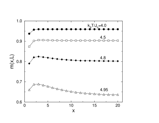
Figure 4: Line magnetization profiles near an edge with opening angle $\theta=\pi/2$ at various temperatures. The couplings are $J_{e}=J_{es}=J_{s}=2J_{b}$. Systems with $40^{3}$ spins have been simulated.

The effect on the edge critical behaviour of weakening the interactions between the edge and the surfaces, $J_{es}$, is demonstrated in Figure 5. A plateau-like behaviour is observed close to $T_{s}$, which facilitates a precise determination of the asymptotic value. Obviously, the value of the critical exponent is non-universal, changing continuously as a function of the coupling strength $J_{es}$, see Table 2. A similar dependency is found when $J_{es}$ is kept fixed whereas $J_{e}$ is changed [10]. The findings of Figure 5 and Table 2 may be related to the reported results on two-dimensional Ising models with a ladder defect [8]. The ladder column corresponds to the edge, and the ladder couplings $J_{l}$ reflect not only the edge-surface interaction $J_{es}$ but also the reduced connectedness to bulk spins at the edge compared to the surfaces. For $J_{es}=J_{e}=J_{s}$, the critical exponent of the edge magnetization has the value $\beta_{2}=0.095\pm 0.005$, significantly lower than the critical exponent of the perfect two-dimensional Ising model, $\beta=1/8$. Of course, the non-monotonic profiles of the line magnetization suggest that a closer analogy between edge properties and descriptions by two-dimensional Ising models with defect lines would require more complicated, extended ladder-type defects.

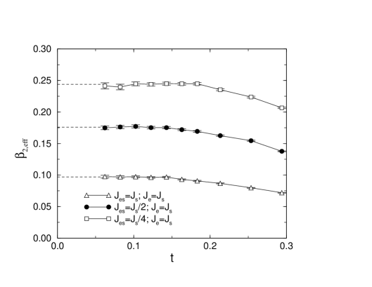
Figure 5: Effective edge exponents as function of the reduced temperature for various values of the coupling $J_{es}$ with $J_{e}=J_{s}=2J_{b}$. Only data not affected by finite-size effects are displayed. The largest system simulated contains $80^{3}$ spins. Error bars result from averaging over several realizations.

Corner criticality in three-dimensional Ising models deserves to be analyzed at the surface transition as well. As edges are local perturbations acting similar to defect lines in two-dimensional models, the corners of a cube may be interpreted as intersection points of three defect lines.

As for the edge, the local magnetization profiles show a non-monotonic behaviour along paths from the edges or corners towards the center of the surface, reflecting the influence of bulk spins. At lower temperatures, the profil is monotonic, with the smallest magnetization at the corners. Close to $T_{s}$, a monotonic behaviour is also expected, with the highest magnetization at the corners. Due to finite-size effects, this last behaviour is not observed in the simulated finite cubes [11].

The analysis of corner magnetization effective exponents yields again critical exponents changing continuously with the strengths of the local couplings, see Table 2. Note that corner criticality has not been studied for the case $J_{es}=J_{s}/4$. Changing corner critical exponents are also observed when varying $J_{e}$ [11]. This non-universal corner criticality is understood by the analogy to two-dimensional Ising models with star defects formed by three intersecting ladder defects [15].

Table 2: Edge and corner magnetization critical exponents $\beta_{2}$ und $\beta_{3}$ at the surface transition for systems with opening angles $\theta=\pi/2$ and $J_{e}=J_{s}=2J_{b}$.

	$J_{es}=J_{s}$	$J_{es}=J_{s}/2$	$J_{es}=J_{s}/4$
$\beta_{2}$	$0.095\pm 0.005$	$0.176\pm 0.005$	$0.244\pm 0.005$
$\beta_{3}$	$0.06\pm 0.01$	$0.26\pm 0.02$

5 Conclusion

Critical phenomena may occur not only in the bulk but also at surfaces, edges, and corners. I have presented results of an extensive Monte Carlo study of edge and corner criticality in three-dimensional Ising systems. At the ordinary transition, edge and corner critical exponents have been computed and compared to analytical predictions. Whereas the critical exponents depend on the wedge angle, they do not depend on microscopic details as the strengths of the local couplings. This is different at the surface transition where coupling dependent edge and corner critical exponents are observed. This non-universal behaviour is understood by analogy with exact results on two-dimensional Ising models with defect lines.

References

- [1] K. Binder, in Phase Transitions and Critical Phenomena, Volume 8 (C. Domb and J. L. Lebowitz, eds.), Academic Press, London, and New York (1983).
- [2] H. W. Diehl, in Phase Transitions and Critical Phenomena, Volume 10 (C. Domb and J. L. Lebowitz, eds.), Academic Press, London, and New York (1986); H. W. Diehl, Int. J. Mod. Phys. B 11, 3503 (1997).
- [3] H. Dosch, Critical Phanomena at Surfaces and Interfaces, Springer, Berlin, Heidelberg, and New York (1992).
- [4] K. Binder and D. P. Landau, Phys. Rev. Lett. 52, 318 (1984).
- [5] C. Ruge, S. Dunkelmann, F. Wagner, and J. Wulf, J. Stat. Phys. 73, 293 (1993).
- [6] J. L. Cardy, J. Phys. A 16, 3617 (1983).
- [7] F. Iglói, I. Peschel, and L. Turban, Adv. Phys. 42, 683 (1993).
- [8] R. Z. Bariev, Sov. Phys. JETP 50, 613 (1979).
- [9] M. Pleimling and W. Selke, Eur. Phys. J. B 5, 805 (1998).
- [10] M. Pleimling and W. Selke, Phys. Rev. B 59, 65 (1999).
- [11] M. Pleimling and W. Selke, Phys. Rev. E 61, 933 (2000).
- [12] U. Wolff, Phys. Rev. Lett. 62, 361 (1989).
- [13] M. Pleimling and W. Selke, Eur. Phys. J. B 1, 385 (1998).
- [14] A. J. Guttmann and G. M. Torrie, J. Phys. A 17, 3539 (1984).
- [15] M. Henkel and A. Patkós, J. Phys. A 21, L231 (1988).