Abstract

The behavior of the subsystem of hydrogen atoms of the KIO${}_{3}\cdot$HIO₃ crystal, whose IR absorption spectra exhibit equidistant submaxima in the vicinity of the maxima in the frequency range of stretching and bending vibrations of OH bonds is studied in the present work. It is shown that hydrogen atoms co-operate in peculiar clusters in which, however, the hydrogen atoms do not move from their equilibrium positions, but become to vibrate synchronously. The interaction between the hydrogen atoms is associated with the overlapping their matter waves, or more exactly, the waves’ substructure, a very light quasi-particles called inertons, which play the basic role in submicroscopic quantum mechanics that has recently been constructed by the author. The exchange by inertons results in the oscillation of hydrogen atoms in clusters, which emerges in the mentioned spectra. The number of atoms, which compose the cluster, is calculated.

arXiv.org e-print archive cond-mat/0108417

Collective dynamics of hydrogen atoms in the KIO${}_{3}\cdot$HIO₃ crystal dictated by a substructure of the hydrogen atoms’ matter waves

PACS: 03.75.-b Matter waves;  34.10+x General theories and models of atomic and molecular collisions and interactions (including statistical theories, transition state, stochastic and trajectory models, etc.);   14.80.-j Other particles (including hypothetical)

Key words: statistical mechanics, clusters, hydrogen structures, interparticle interaction, matter waves, inertons, IR spectra

1. Statement of the problem

This work presents a manifold research, which embraces the experimental results by Puchkovska and collaborators [1] on a very peculiar behavior of hydrogen atoms in the $\delta$-KIO${}_{3}\cdot$HIO₃ crystal, a rather new concept of the clustering, which appears at the statistical mechanical description of interacting particles, first proposed by Belotsky and Lev [2] (see also Refs. [3-5]) and submicroscopic quantum mechanics developed in the real space, which has recently been constructed by the author [6-13].

Below the major experimental results obtained [1,14-16] on the delta modification of the KIO${}_{3}\cdot$HIO₃ crystal is described. In particular, the FT-IR absorption spectra of powdered samples in the frequency range of stretching and bending vibrations of OH bonds are analyzed. Since the spectroscopic studies reveal a modulation of the spectral bands, this effect is associated with collective vibrations of hydrogen atoms. Such a behavior is possible only in the case when the hydrogen atoms represent a dynamic system of a sort. To study this possibility, we should first have the rigorous evidence that the behavior of hydrogen atoms, or protons are distinguished from the backbone atoms. Note that this the subject of study that Fillaux and collaborators have been conducting for decade [17-22]: Using the incoherent inelastic neutron scattering technique they have investigated vibrational dynamics for protons in various solids and revealed that proton dynamics is almost totally decoupled from surrounding heavy atoms. Besides, Fillaux noted that the proton subsystem demonstrates a collective dynamics (see also Trommsdorff et al. [23,24], who disclosed the coherent proton tunneling and cooperative proton tunneling and transfer of four protons in hydrogen bonds of benzoic acids crystals).

The statistical mechanical approach proposed in Refs. [2-5] makes allowance for spatial nonhomogeneous states of interacting particles in the system studied. However, in the case when the inverse operator of the interaction energy cannot be determined one should search for the other method, which, nevertheless, will make it possible to take into account a plausible nonhomogeneous particle distribution. In papers [2-5] systems of interacting particles have been treated from the same standpoint [1], however, the number of variables describing the systems in question has been reduced and a new canonical variable, which characterized the nascent nonhomogeneous state (i.e. cluster), automatically aroused as a logical consequence of the behavior of particles. A detailed analysis of the appearance of nonhomogeneous states in systems of interacting particles submitted to quantum statistics (Fermi’s and Bose’) has been performed in Ref. [5]. In the present work we will consider a possible clustering of hydrogen atoms in the KIO${}_{3}\cdot$HIO₃ crystal in the framework of Boltzmann statistics based on ideas developed in Refs. [2-5]. If we are able to form a cluster of hydrogen atoms, this automatically will mean that the hydrogen atoms fall within proper vibrations, which should be distinguished from the spectra of heavy atoms. Thus, if clusters of hydrogen atoms exist, each of them will represent a typical dynamic system and therefore vibrations of hydrogen atoms being superimposed on the carrying absorption OH bands will induce a modulation of the OH bands, which has been reveled in the experiment [1].

What kind of a problem can one meet at such a consideration? The said approach can bring about clusters only in the case when repulsive and attractive components of the pair potential feature very different dependencies on distance from the particle. However, we can not expect that the electromagnetic interaction between hydrogen atoms in the crystal can exhibit a great difference between repulsive and attractive components of the pair potential (for example, for the Van der Waals interaction the behavior of the components, respectively $1/r^{12}$ and $1/r^{6}$, are not fundamentally different).

It has been shown in the author works devoted to the foundations of quantum mechanics [6-13] that the matter waves of particles are characterized by a certain substructure, namely, that the matter waves come from the interaction of a moving particle with a space substrate, i.e. real space. Due to the interaction, an ensemble of sub quasi-particles should appear surrounding the particle (these quasi-particles were called ”inertons” [6], as they represent inert properties of canonical particles). A cloud of inertons spreads around the particle in the range

$$\Lambda=\lambda{\kern 1.0pt}{\kern 1.0pt}c/v$$ (1)

where $\lambda$ is the particle’s de Broglie wavelength, $v$ and c are velocities of the particle and light, respectively. Thus the wave $\psi$-function becomes determined in the range around the particle covered by the amplitude of inerton cloud (1). Submicroscopic mechanics developed in the real space [6-13] makes it possible to overcome all conceptual difficulties inherent in orthodox statistical quantum mechanics (developed in an abstract space) and at the same time submicroscopic mechanics has easily fitted into Schrödinger’s [6,7] and Dirac’s [9] formalisms accounting for the inner reason of allegedly different prerequisites for the two approaches [9,12]. A great number of experimental manifestations of clouds of inertons surrounding electrons was demonstrated in Ref. [10]. Our own prediction and experimental verification of the existence of inertons were stated in paper [8].

In the present work we shall use one consequence, which directly follows from the theory [6-13] and which has already been employed in papers [5,8]. Clouds of inertons expended around the same particles (for instance, hydrogen atoms) are exemplified by the same characteristics, namely: amplitude (1), mass, momentum, and energy. This means that a system of such clouds should interact much as elastic balls and, therefore, the potential energy of the interacting clouds may be written as $\gamma{\kern 1.0pt}r^{2}/2$ where $r$ is a deviation of an atom from its equilibrium position in the lattice and $\gamma$ is an elasticity, or force, constant of the lattice’s inerton field.

Keeping in mind the aforesaid, let us now turn to a close examination of the behavior of hydrogen atoms in the KIO${}_{3}\cdot$HIO₃ crystal.

2. Peculiarities experimentally revealed in hydrogen atoms dynamics

The crystal structure, proton disorder and low temperature phase transition of the $\delta$-KIO${}_{3}\cdot$HIO₃ crystal have been studied by means of X-ray diffraction, dielectric, calorimetric and FT-IR and FT-Raman techniques by Engelen et al. [14]. It has been found that [I₃O₉H_3/2]^-3/2 ions are linked by means of hydrogen bonds to the oxygen atom at the middle of two other [I₃O₉H_3/2]^-3/2 anions. Moreover, hydrogen-bonded plane grids parallel (100) are formed with hydrogen bonded chains in [011]. K⁺ ion is located between the plane grids and completes the crystal structure of $\delta$-KIO${}_{3}\cdot$HIO₃. Basically, in the crystal studied hydrogen bonds do not form an entire uninterrupted network, but rather represent local islands and each of them features a compact ordered system of hydrogen bonds.

Further experimental studies conducted by Puchkovska and collaborators [14,1] have been aimed at the detailed measurements of the FT-IR absorption spectra of the powdered $\delta$-KIO${}_{3}\cdot$HIO₃ crystal in the frequency range of stretching and bending vibrations of OH bonds for the temperature range from 13 to 293 K. The spectra recorded in high-frequency region are shown in Figs. 1 and 2. Hydrogen bonds in the crystal under consideration were ascribed to weak and medium hydrogen bonds. For such hydrogen bonds Fermi resonance does not practically excite $\nu$(OH) spectral band shape [25]. However, the presence of K_3/2[I₃O₉H_3/2] moieties is the major structural feature of the $\delta$-KIO${}_{3}\cdot$HIO₃, which are able to induce a similar distribution observed in the $\nu$(OH) band for $\alpha$-HIO₃ crystal [16].

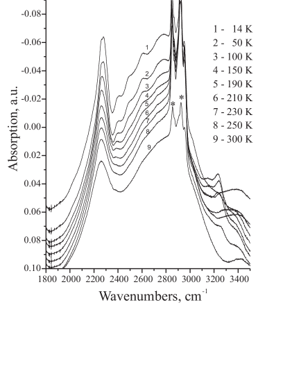
Figure 1: Temperature dependent IR spectra of polycrystalline $\delta$-KIO${}_{3}\cdot$HIO₃ (suspension in Nujol) in the region of stretching $\nu$(OH) mode. Asterics denote the Nujol absorption bands. (With permission from Ref. [1].)

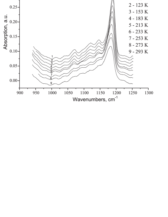
Figure 2: Temperature dependent IR spectra of polycrystalline $\delta$-KIO${}_{3}\cdot$HIO₃ in NaCl pellet in the region of the in-plane bending mode $\delta$(OH).(With permission from Ref. [1].)

A very strong broad band centered at 2900 cm^-1 and less intensive band at 2320 cm^-1 have been assigned [14] to $\nu$(OH) stretching vibration and $2\delta$(OH) overtone, respectively. In the 1000 to 1300 cm^-1 region there is a band of the medium intensity with peak position 1185 cm^-1 at the room temperature; the frequencies belong to the in-plane bending modes $\delta$(OH) of I – O – H$\cdot\cdot\cdot$O – I fragments. The temperature dependencies of the peak position and half-width of the $\delta$(OH) band were measured in work [16] and showed sharp changes in their slopes near 220 K. This was associated with the phase transition in the proton sublattice of order-disorder type.

The most interesting result reported in Refs. [14,1] is the disclosure of a pronounced ”modulation” in both low-frequency slopes and high-frequency ones of the $\nu$(OH) and $\delta$(OH) bands especially at temperature below 220 K (Figs. 1 and 2). However, the substructure is only slightly distinguished in the low-frequency slopes. The frequencies of the $\delta$(OH) band satellites at 99 K are 1148, 1120, 1095, 1068, 1040, 1011, 982, 956, and 932 cm^-1. The differences between the succeeding peaks in this progression are almost constant that equals to $24.5\pm 6$ cm^-1. The $\nu$(OH) band satellites in the spectra below 220 K are located at the frequencies 2780, 2670, 2560, and 2445 cm^-1 and the respective difference between the maximums is near $120\pm 10$ cm^-1. When passing from higher to lower temperatures, all the bands become sharper. At the same time their relative positions and intensities are still retained. Note that a similar band progression has also been observed for the $\nu$(OH) and $\delta$(OH) bands in the spectra of $\alpha$-HIO₃ [15] and $\alpha$-KIO${}_{3}\cdot$HIO₃ [16] crystals.

The origin of such an unusual spectroscopic feature cannot be associated with any possible strong anharmonic coupling between the high-frequency vibrational modes of hydrogen bonds and low-frequency lattice phonons as it was described in Ref. [26]. According to their theoretical model the appearance of a multiband substructure at the low frequency slope of the $\nu$(OH) absorption band in a solid is possible only in situations of strong and very strong hydrogen bonds. However, this is not the case for the crystal in question where only weak and medium strong hydrogen bonds are present.

Taking into account the complex structure of the given crystal ($Z=24$), proton order for $T<T_{c}$ and the data on practically independence of proton dynamics in solids, Fillaux et al. [17-22], a radically new theory of the proton behavior can be proposed.

3. Clusterization in the framework of orthodox statistical mechanics

Having considered whether nonhomogeneous states, i.e. clusters, may appear spontaneously in systems with hydrogen bonds, we first should describe the methodology developed in Refs. [3-5] and then apply it to the case, which falls within the Boltzmann statistics. We shall start from the construction of the Hamiltonian for a system of interacting particles. The Hamiltonian can be represented as follows

$$H\left({n}\right)=\sum\limits_{s}{E_{s}}n_{s}-\tfrac{{1}}{{2}}\sum\limits_{s,{\kern 1.0pt}{\kern 1.0pt}{s}^{\prime}}{V_{s{\kern 1.0pt}{s}^{\prime}}{\kern 1.0pt}n_{s}{\kern 1.0pt}n_{{s}^{\prime}}+\tfrac{{1}}{{2}}\sum\limits_{s,{\kern 1.0pt}{\kern 1.0pt}{s}^{\prime}}{U_{s{\kern 1.0pt}{s}^{\prime}}{\kern 1.0pt}n_{s}{\kern 1.0pt}n_{{s}^{\prime}}}}$$ (2)

where E_s is the additive part of the particle energy in the sth state. The main point of the approach is the presentation of the total atom/molecular pair potential into two terms: the repulsion and attraction components. So, in the Hamiltonian (2) V${}_{ss^{\prime}}$ and U${}_{ss^{\prime\prime}}$ are respectively the paired energies of attraction and repulsion between particles located in the states s and $s^{\kern 1.0pt\prime}$. It should be noted that the signs before the potentials in expression (2) specify proper signs of the attractive and repulsive paired energies and this means that both functions V${}_{ss^{\prime}}$ and U${}_{ss^{\prime}}$ in expression (2) are positive. The statistical sum of the system

$$Z=\sum\limits_{\{n\}}{\exp\left({-H\left({n}\right)/k_{{\kern 1.0pt}\rm B}T}\right)}$$ (3)

may be presented in the field form

$$Z = \int_{-\infty}^{\infty}D{\kern 1.0pt}\phi\int_{-\infty}^{\infty}D{\kern 1.0pt}\psi\sum\limits_{\{n\}}\exp\Big{[}\sum\limits_{s}\Big{(}\psi_{s}+i\phi_{s}\Big{)}{\kern 1.0pt}{\kern 1.0pt}n_{s}$$

$$- \tfrac{1}{2}\sum\limits_{s,{\kern 1.0pt}{s}^{\prime}}\Big{(}{\tilde{U}_{s{\kern 1.0pt}{s}^{\prime}}^{-1}{\kern 1.0pt}\phi_{s}{\kern 1.0pt}\phi_{{s}^{\prime}}+\tilde{V}_{s{\kern 1.0pt}{s}^{\prime}}^{-1}{\kern 1.0pt}\psi_{s}{\kern 1.0pt}\psi_{{s}^{\prime}}}\Big{)}\Big{]}$$

due to the following representation known from the theory of Gauss integrals

$$\exp\left({\frac{{\rho^{2}}}{{2}}\sum\limits_{s,{\kern 1.0pt}{\kern 1.0pt}{s}^{\prime}}{\mathcal{W}_{s{\kern 1.0pt}{s}^{\prime}}{\kern 1.0pt}n_{s}{\kern 1.0pt}n_{{s}^{\prime}}}}\right)$$ (5)

$$\quad\quad={\rm Re}\int_{-\infty}^{\infty}D{\kern 1.0pt}{\kern 1.0pt}\vartheta\exp\left[{\rho\sum\limits_{s}{n_{s}\vartheta_{s}-\tfrac{{1}}{{2}}\sum\limits_{s,{\kern 1.0pt}{\kern 1.0pt}{s}^{\prime}}{\mathcal{W}_{s{\kern 1.0pt}{s}^{\prime}}^{-1}\vartheta_{s}\vartheta_{{s}^{\prime}}}}}\right]$$

where $D{\kern 1.0pt}{\kern 1.0pt}\vartheta\equiv\prod\nolimits_{s}{\sqrt{{\rm det}||\mathcal{W}_{s{\kern 1.0pt}{s}^{\prime}}||}}\sqrt{2\pi}{\kern 1.0pt}d{\kern 1.0pt}\vartheta_{s}$ implies the functional integration with respect to the field $\vartheta$; $\rho^{2}=\pm 1$ in relation to the sign of interaction (+1 for attraction and $-1$ for repulsion). The dimensionless energy parameters $\tilde{V}_{s{\kern 1.0pt}{s}^{\prime}}=V_{s{\kern 1.0pt}{s}^{\prime}}/k_{\rm{\kern 1.0pt}B}T,\quad\tilde{U}_{s{\kern 1.0pt}{s}^{\prime}}=U_{s{\kern 1.0pt}{s}^{\prime}}/k_{\rm{\kern 1.0pt}B}T,$ and $\tilde{E}_{s}/k_{\rm{\kern 1.0pt}B}T$ are introduced into expression (4). Further, we will use the known formula

$$\frac{{1}}{{2\pi{\kern 1.0pt}i\quad}}\oint{d{\kern 1.0pt}z}{\kern 1.0pt}{\kern 1.0pt}z^{{\kern 1.0pt}{\kern 1.0pt}N-1-\sum\nolimits_{s}{n_{s}}}=1,$$ (6)

which makes it possible to settle the quantity of particles in the system, $\sum\nolimits_{s}{n_{s}=N},$ and, consequently, we can pass to the consideration of the canonical ensemble of N particles. Thus the statistical sum (4) is replaced for

$$\begin{array}[]{l}Z={\rm Re}\frac{1}{2\pi i}\oint{d{\kern 1.0pt}z}\int{D\phi\int{D\psi{\kern 1.0pt}\exp\{-\tfrac{{1}}{{2}}\sum\limits_{s,{\kern 1.0pt}{\kern 1.0pt}{s}^{\prime}}{\left({\tilde{U}_{s{\kern 1.0pt}{s}^{\prime}}^{-1}{\kern 1.0pt}{\kern 1.0pt}\phi_{s}{\kern 1.0pt}\phi_{{s}^{\prime}}+\tilde{V}_{s{\kern 1.0pt}{s}^{\prime}}^{-1}{\kern 1.0pt}\psi_{s}{\kern 1.0pt}\psi_{{s}^{\prime}}}\right)}}}\\ \quad\quad+\left({N-1}\right){\kern 1.0pt}{\kern 1.0pt}{\kern 1.0pt}{\kern 1.0pt}\ln z\}\times\sum\limits_{\{n_{s}\}=0}^{1}{\exp\{\sum\limits_{s}{n_{s}\left({\psi_{s}+i{\kern 1.0pt}\phi_{s}-\tilde{E}_{s}}\right)}-\ln z\}}.\\ \end{array}$$ (7)

Summing over n_s we obtain

$$Z={\rm Re}\frac{{1}}{{2\pi i}}\int{D\phi\int{D\psi\oint{d{\kern 1.0pt}z}}}{\kern 1.0pt}{\kern 1.0pt}e^{{\kern 1.0pt}{\kern 1.0pt}S\left({\phi,{\kern 1.0pt}{\kern 1.0pt}\psi,{\kern 1.0pt}{\kern 1.0pt}z}\right)}$$ (8)

where

$$\begin{array}[]{l}S=\sum\limits_{s}{\left\{{-\tfrac{{1}}{{2}}\sum\limits_{{s}^{\prime}}{\left({\tilde{U}_{s{\kern 1.0pt}{s}^{\prime}}^{-1}{\kern 1.0pt}{\kern 1.0pt}\phi_{s}{\kern 1.0pt}\phi_{{s}^{\prime}}+\tilde{V}_{s{\kern 1.0pt}{s}^{\prime}}^{-1}{\kern 1.0pt}\psi_{s}{\kern 1.0pt}\psi_{{s}^{\prime}}}\right)}}\right.}\\ \left.{\quad\quad+\eta{\kern 1.0pt}{\kern 1.0pt}\ln\left|{1+\frac{{\eta}}{{z}}e^{{\kern 1.0pt}-\tilde{E}_{s}}e^{{\kern 1.0pt}\psi_{s}}\cos\phi_{s}}\right|}\right\}+\left({N-1}\right){\kern 1.0pt}{\kern 1.0pt}{\kern 1.0pt}\ln z.\\ \end{array}$$ (9)

Here, the symbol characterizes the kind of statistics: Bose ($\eta=+1$) or Fermi ($\eta=-1$). Let us set $z=\xi+i{\kern 1.0pt}\zeta$ and consider the action $S$ on a transit path that passes through the saddle-point at a fixed imaginable variable ${\rm Im}z=\zeta_{{\kern 1.0pt}0}.$ In this case $S$ may be regarded as the functional that depends on the two field variables $\phi$ and $\psi$, and the fugacity $\xi=e^{-\mu/k_{{\kern 1.0pt}\rm B}T}$ where $\mu$ is the chemical potential.

In a classical system the mean filling number of the sth energy level obeys the inequality

$$n_{s}=\frac{{1}}{{\xi}}e^{-\tilde{E}_{s}}=e^{\left({\mu-E_{s}}\right)/k_{\rm{\kern 1.0pt}B}T}<<1$$ (10)

(note the chemical potential $\mu<0$ and $|\mu|/k_{\rm{\kern 1.0pt}B}T\gg 1$). By this means, we can simplify expression (9) expanding the logarithm into a Taylor series in respect to the small second member. As a result, we get the action that describes the ensemble of interacting particles, which are subjected to the Boltzmann statistics

$$\begin{array}[]{l}S\cong\sum\limits_{s}{\left\{{-\tfrac{{1}}{{2}}\sum\limits_{{s}^{\prime}}{\left({\tilde{U}_{s{\kern 1.0pt}{s}^{\prime}}^{-1}{\kern 1.0pt}{\kern 1.0pt}\phi_{s}{\kern 1.0pt}\phi_{{s}^{\prime}}+\tilde{V}_{s{\kern 1.0pt}{s}^{\prime}}^{-1}{\kern 1.0pt}\psi_{s}{\kern 1.0pt}\psi_{{s}^{\prime}}}\right)+\frac{{1}}{{\xi}}e^{-\tilde{E}_{s}}e^{\psi_{s}}\cos\phi_{s}}}\right\}}\\ \quad\quad+\left({N-1}\right)\ln\xi.\\ \end{array}$$ (11)

The extremum of functional (11) is realized at the solutions of the equations $\delta{\kern 1.0pt}S/\delta\phi=0,\quad\delta{\kern 1.0pt}S/\delta{\kern 1.0pt}\psi=0,$ and $\delta{\kern 1.0pt}S/\delta\xi=0$, or explicitly

$$\sum\limits_{{s}^{\prime}}{\tilde{U}_{{s}^{\prime}}^{-1}}\phi_{{s}^{\prime}}=-\frac{1}{{\xi}}{\kern 2.0pt}e^{-\tilde{E}_{s}}e^{\psi_{s}}\sin\phi_{s},$$ (12)

$$\sum\limits_{{s}^{\prime}}{\tilde{V}_{{s}^{\prime}}^{-1}}\psi_{{s}^{\prime}}=-\frac{1}{{\xi}}{\kern 2.0pt}e^{-\tilde{E}_{s}}e^{\psi_{s}}\cos\phi_{s},$$ (13)

$$\frac{{1}}{{\xi}}\sum\limits_{{s}^{\prime}}{e^{-\tilde{E}_{{s}^{\prime}}}e{\kern 1.0pt}^{\psi_{{s}^{\prime}}}\cos\phi_{{s}^{\prime}}}=N-1.$$ (14)

If we introduce the denotation

$$\mathcal{N}_{s}=\frac{1}{\xi}{\kern 1.0pt}{\kern 1.0pt}e^{-\tilde{E}_{s}}e^{\psi_{s}}\cos\phi_{s},$$ (15)

we will easily see from Eq. (15) that the sum $\sum\nolimits_{s}{\mathcal{N}_{s}}$ is equal to the number of particles in the system studied. So the combined variable $\mathcal{N}_{s}$ specifies the quantity of particles in the sth state. This means that one may treat $\mathcal{N}_{s}$ as the variable of particle number in a cluster. Using this variable, we can represent the action (11) as a function of only one variable $\mathcal{N}_{s}$ and the fugacity $\xi$

$$\begin{array}[]{l}S=-\sum\limits_{s,{\kern 1.0pt}{\kern 1.0pt}{s}^{\prime}}{\left[{\tilde{V}_{s{\kern 1.0pt}{s}^{\prime}}{\kern 1.0pt}\mathcal{N}_{s}{\kern 1.0pt}\mathcal{N}_{{s}^{\prime}}+\tilde{U}_{s{\kern 1.0pt}{s}^{\prime}}{\kern 1.0pt}\mathcal{N}_{s}{\kern 1.0pt}\mathcal{N}_{{s}^{\prime}}\left({\frac{{e^{-2\tilde{E}_{s}+2\sum\nolimits_{{s}^{\prime}}{\tilde{V}_{s{\kern 1.0pt}{s}^{\prime}}\mathcal{N}_{{s}^{\prime}}}}}}{{\xi^{2}\mathcal{N}_{s}^{2}}}-1}\right)}\right]}\\ \quad\quad+\sum\limits_{s}{\mathcal{N}_{s}{\kern 1.0pt}{\kern 1.0pt}\left({1+\ln\xi}\right)}.\\ \end{array}$$ (16)

If we put the variable $\mathcal{N}_{s}=\mathcal{N}=\rm const$ in each of clusters, we may write instead of Eq. (14)

$$\mathcal{N}K=N-1.$$ (17)

Here K is the quantity of clusters and $\mathcal{N}$ is classified as the number of particles in a cluster. Thus the model deals with particles entirely distributed by clusters.

It is convenient now to pass to the consideration of one cluster and change the discrete approximation to a continuous one. The transformation means the passage from the summation over discrete functions in expression (15) to the integration of continual functions by the rule

$$\begin{array}[]{l}\sum\nolimits_{s}{f_{s}=\frac{{1}}{{\mathcal{V}}}{\kern 1.0pt}\int\limits_{\rm cluster}{d{\kern 1.0pt}\vec{x}}{\kern 1.0pt}f\left({\vec{x}}\right){\kern 1.0pt}{\kern 1.0pt}}=\frac{{1}}{{\mathcal{V}}}{\kern 1.0pt}{\kern 1.0pt}\int\limits_{0}^{2\pi}{d{\kern 1.0pt}{\kern 1.0pt}\phi}\int\limits_{0}^{\pi}{d{\kern 1.0pt}\theta}\sin\theta\int\limits_{1}^{R/g}{d{\kern 1.0pt}{\kern 1.0pt}x}{\kern 1.0pt}{\kern 1.0pt}x^{2}f\left({x}\right)\\ \quad\quad\quad{\kern 1.0pt}={\kern 1.0pt}{\kern 1.0pt}{\kern 1.0pt}3\int\limits_{1}^{\mathcal{N}^{1/3}}{d{\kern 1.0pt}{\kern 1.0pt}x}{\kern 1.0pt}{\kern 1.0pt}x^{2}f\left({x}\right);\end{array}$$ (18)

here $\mathcal{V}=4\pi{\kern 1.0pt}g^{3}/3$ is the effective volume of one particle, $R/{\kern 1.0pt}g$ is the dimensionless radius of a cluster where g is the mean distance between particles in a cluster, and x is the dimensionless variable ($x=\left[{1,{\kern 1.0pt}\;R/g}\right]$); therefore, the number of particles in the cluster is linked with $R$ and $g$ by the relation $\left({R/g}\right)^{3}=\mathcal{N}$ (see Ref. [4] for details). Below we assume that $\mathcal{N}\gg 1$.

If we introduce the designations ($x$ is the dimensionless variable)

$$a=3{\kern 1.0pt}\int_{1}^{\mathcal{N}^{1/3}}{d{\kern 1.0pt}x{\kern 1.0pt}{\kern 1.0pt}}x^{2}{\kern 1.0pt}\tilde{U}(x),\quad\;\;\;\quad\quad\quad b=3{\kern 1.0pt}\int_{1}^{\mathcal{N}^{1/3}}{d{\kern 1.0pt}x{\kern 1.0pt}{\kern 1.0pt}}x^{2}{\kern 1.0pt}\tilde{V}(x),$$ (19)

we will arrive at the action in the simple form

$$S=K\cdot\Big{\{}\left({a-b}\right)\mathcal{N}^{\kern 1.0pt2}-\frac{{1}}{{\xi^{2}}}{\kern 1.0pt}a{\kern 1.0pt}e^{-2\tilde{E}+2b\mathcal{N}}\Big{\}}+(N-1)\ln\xi.$$ (20)

The exponent term in the right-hand side of expression (20) is the smallest one (owing to the inequality $e^{-2\tilde{E}}/\xi{\kern 1.0pt}^{2}{\kern 1.0pt}\ll 1$) and we omit it hereinafter. Thus we shall start from the action

$$S\simeq K\cdot\Big{\{}\left({a-b}\right)\mathcal{N}^{\kern 1.0pt2}+\mathcal{N}\ln\xi\Big{\}}.$$ (21)

The extremum (minimum) of the action (21) is reached at the meaning of $\mathcal{N},$ which is found from the equation $\delta S/\delta\mathcal{N}=0$ and satisfies the inequality $\partial^{{\kern 1.0pt}2}S/\delta\mathcal{N}^{{\kern 1.0pt}2}>0.$ The value of $\mathcal{N}_{\rm extr}$ obtained in such a way will correspond to the number of particles that compose a cluster.

4. Collective dynamics of hydrogen atoms

In the $\delta$-KIO${}_{3}\cdot$HIO₃ crystal hydrogen atoms are not free, they are bound with oxygen atoms. That is why we should analyze, what kinds of clusters could hydrogen atoms form? In the first approximation, in the crystal lattice atoms/molecules are characterized by their harmonic vibrations in the vicinity of equilibrium positions. The amplitude of small displacement A of an atom in the crystal lattice lies in the range 0.01 to 0.03 nm. In the crystal state this parameter, i.e. A, surrogates the de Broglie wavelength $\lambda$ of a free atom. Since A takes the place of $\lambda$, the expression for the amplitude of inerton cloud (1) becomes $\Lambda=A{\kern 1.0pt}c/\upsilon$. That is, $\Lambda\sim 1\;{\kern 1.0pt}{\kern 1.0pt}\mu$m and therefore the inerton cloud of a crystal’s entity can span over $10^{{\kern 1.0pt}3}g$, where g is the lattice constant. The general form of $A$ in the crystal with $N$ atoms is $A_{l}=l/gN$ where $l=2,{\kern 3.0pt}3,{\kern 3.0pt}...,(N-1)$, that is $A_{l}$ is the wavelength of the $l$th mode of the acoustic spectrum of the crystal. Note that such a strong overlap of inerton clouds of entities, in particular, protons, is permanently used in the theory of ferroelectrics for a long time: researchers implicitly introduce an order parameter that introduces long-range interaction in the proton subsystem below the phase transition that is needed for the description of the ferro- or antiferroelectric state, though the de Broglie wavelength of protons has only an order of the lattice constant $g$ (see, e.g. Refs. [27,28]).

The methodology, which is described, does not need any fitting order parameter. Instead, based on the findings of Fillaux et al. [17-22] (especially see review article [21]), we can consider the subsystem of hydrogen atoms as quite independent from the framework. This is quite possible to do if we use the two-level model for the description of hydrogen atoms; in the model each hydrogen atom is able to occupy either the ground state or only one excited state. Being in the excited state, the hydrogen atoms will behave as typical quasi-particles, which are able to interact each other. Due to the link with oxygens, the interaction between the hydrogen atoms is rather Van der Waals’ and can be simulated by the Lennard-Jones potential. The second type of interaction does not fall within the electromagnetic interaction and can be assigned to the pure quantum mechanical interaction caused by the overlapping of the hydrogen atoms’ matter waves, i.e. elastic inerton clouds.

Thus, the pair potential between hydrogen atoms can be written as the sum of the Lennard-Jones potential and an additional harmonic potential that takes into account the weak quantum mechanical interaction of hydrogen atoms via the inerton field on the scale $r\ll\Lambda$:

$$W=\epsilon\left[{\left({\frac{{1}}{{r/g}}}\right)^{12}-{\kern 1.0pt}{\kern 1.0pt}{\kern 1.0pt}{\kern 1.0pt}\left({\frac{{1}}{{r/g}}}\right)^{{\kern 1.0pt}6}}\right]+\tfrac{1}{2}{\kern 1.0pt}{\kern 1.0pt}\gamma{\kern 1.0pt}r^{{\kern 1.0pt}2}.$$ (22)

Here $\epsilon$ is the energy constant, $g$ is the equilibrium distance between a pair of interacting hydrogen atoms and $\gamma$ is the elasticity constant that characterizes the elastic interaction of hydrogen atoms’ inerton clouds (and may be partly the backbone atoms).

Once again, why the potential is chosen in the form $\tfrac{1}{2}{\kern 1.0pt}\gamma{\kern 1.0pt}r^{{\kern 1.0pt}2}$? This is potential energy that characterizes oscillations of H-atoms near their equilibrium positions; here $r$ is the difference between positions of a pair of H-atoms. Therefore in this expression $r$ plays a role of the de Broglie wavelength of a H-atom, or a group of collective vibrating H-atoms (in the latter case $r$ represents a typical acoustic wavelength).

Let us now separate repulsive and attractive parts from the potential (22) and represent them in the dimensionless form

$$\tilde{U}\left({x}\right)=\frac{{\epsilon}}{{k_{{\kern 1.0pt}\rm B}T}}{\kern 1.0pt}\frac{{1}}{{x^{12}}},$$ (23)

$$\tilde{V}\left({x}\right)=\frac{{\epsilon}}{{k_{{\kern 1.0pt}\rm B}T}}{\kern 1.0pt}\frac{{1}}{{x^{6}}}-\frac{{\gamma{\kern 1.5pt}\delta g^{2}}}{{2{\kern 1.0pt}k_{{\kern 1.0pt}\rm B}T}}{\kern 1.5pt}x^{2}$$ (24)

where $\delta g$ is the amplitude of local deviation of a H-atom from its equilibrium position (once again, $\delta g$ is the de Broglie wavelength of an atom in a solid).

Substituting potentials (23) and (24) into the corresponding formulas for parameters a and b (19), we get instead of expression (21) with accuracy to $1/\mathcal{N}$

$$S=K\cdot\Big{\{}\Big{(}36\frac{\epsilon}{k_{\rm B}T}-\frac{3}{10}\frac{\gamma{\kern 1.5pt}\delta g^{{\kern 1.0pt}2}}{k_{\rm B}T}\mathcal{N}^{{\kern 1.0pt}5/3}\Big{)}\mathcal{N}^{{\kern 1.0pt}2}+\mathcal{N}\ln\xi\Big{\}}.$$ (25)

If we retain the major terms in the equation $\delta S/\delta\mathcal{N}=0,$ we will obtain retaining highest terms

$$72{\kern 1.0pt}{\kern 1.0pt}\frac{\epsilon}{k_{\rm B}T}{\kern 1.0pt}\mathcal{N}-\frac{11}{10}{\kern 1.0pt}\frac{\gamma{\kern 1.5pt}\delta g^{2}}{k_{\rm B}T}{\kern 1.0pt}\mathcal{N}^{{\kern 2.0pt}8/3}\cong 0.$$ (26)

The solution to equation (26) is

$$\mathcal{N}=\left(\frac{11}{720}{\kern 2.0pt}\frac{\epsilon}{\gamma{\kern 1.5pt}\delta g^{2}}\right)^{3/5}.$$ (27)

Here the interaction energy between a pair of hydrogen atoms is taken to be typical Van der Waals’, i.e. $\epsilon\simeq 10$ kJ/mol $\equiv 1.66\times 10^{-20}$ J; the amplitude of deviation of a H-atom from the equilibrium position in a hydrogen cluster studied can be put equal to $\delta g=0.2\times 10^{-10}$ m; the elasticity constant of the hydrogen atoms’ inerton field, i.e. $\gamma$, is a free parameter; let us set $\gamma=8.8$ N/m (on average, the force constant in a solid comes out to several tens of N/m).

Substituting the aforementioned numerical values of $\epsilon$, $\delta g$ and $\gamma$ into expression (27) we obtain: $\mathcal{N}=52$.

The value of hydrogen atoms $\cal N$ is also evident from the spectra shown in Figs. 1 and 2. Indeed, it is obvious that our cluster is some kind of a dynamic system, because hydrogen atoms, which enter the cluster, do not move from their equilibrium positions, but only trade inerton excitations. In other words, we may treat the cluster as a crystallite in which H-atoms vibrate by the rule typical for an usual crystallite: The kinetic energy of H-atoms periodically passes to the potential one. On the microscopic level this means that the inert mass of each of the hydrogen atoms fluctuate periodically changing from $m_{{\kern 1.0pt}{\rm H}}-\frac{1}{2}m^{*}$ to $m_{{\kern 1.0pt}{\rm H}}+\frac{1}{2}m^{\ast}$, where $m^{\ast}$ is the effective mass of an inerton excitation in the crystallite studied (in other words, the vibratory motion of hydrogen atoms might be modulated by the oscillation of the mass of the crystallite lattice’s sites).

Inertons carry mass and feature velocity. Because of that, the behavior of inerton excitations in the crystallite can be studied starting from the Lagrangian that is typical for the crystal lattice of a solid (see, e.g. Ref. [30])

$$L=\frac{m_{\rm H}}{2}\sum\limits_{{\bf l};{\kern 1.0pt}{\kern 1.0pt}{\kern 1.0pt}\alpha}{\dot{u}_{{\kern 1.0pt}{\bf l}{\kern 1.0pt}\alpha}^{2}-}{\kern 1.0pt}{\kern 1.0pt}{\kern 1.0pt}\frac{1}{2}{\kern 1.0pt}{\kern 1.0pt}{\sum\limits_{{\bf l},{\bf n};{\kern 1.0pt}\alpha,\beta}}^{\prime}{\kern 2.0pt}{\kern 1.0pt}\gamma_{\alpha{\kern 1.0pt}\beta}{\kern 1.0pt}\left({{\bf l}-{\bf n}}\right){\kern 1.0pt}{\kern 1.0pt}u_{{\kern 1.0pt}{\bf l}{\kern 1.0pt}\alpha}u_{{\kern 1.0pt}{\bf n}{\kern 1.0pt}\beta}.$$ (28)

Here the first term describes the kinetic energy of H-atoms and the second term specifies their potential energy. The prime at the sum symbol in Lagrangian (28) signifies that terms with coinciding indices l and n are not taken into account in summation. $u_{\kern 1.0pt\bf l{\kern 1.0pt\kern 1.0pt}\alpha}$ $(\alpha=1,{\kern 1.0pt}2,{\kern 1.0pt}3)$ are three components of displacement of a H-atom from the crystallite site whose equilibrium position is determined by the lattice vector l; $\dot{u}_{{\kern 1.0pt}{\bf l}{\kern 1.0pt\kern 1.0pt}\alpha}$ are three components of the velocity of the H-atom; $\gamma_{\alpha{\kern 1.0pt}\beta}{\kern 1.0pt}\left({\bf l-n}\right)$ are the components of the elasticity tensor of the crystallite lattice and then the elasticity constant $\gamma$ that enters into expressions from (22) to (27) can be considered as the convolution of the tensor $\gamma_{\alpha\beta}$.

Let us now approximate the elasticity tensor $\gamma_{\alpha\beta}$ by two components: longitudinal, $\gamma_{||}$, and transversal, $\gamma_{\bot}$.

The Lagrangian (28) produces the dispersion equation for allowed frequencies of excitations in a cluster. The form of the equation is the same as that for pure acoustic phonon branches in a solid (see e.g. Ref. [29])

$$\omega_{\ell,\kern 1.0ptj}\cong q_{j}{\kern 2.0pt}g{\kern 1.0pt}\sqrt{\gamma_{\ell}{\kern 0.5pt}/m_{\rm H}}=q_{j}{\kern 1.0pt}{\kern 2.0pt}v_{\ell}$$ (29)

where $g\approx 0.3$ nm is the lattice constant (the typical distance between hydrogen atoms in a hydrogen cluster); the index $\ell$ characterizes the two types of inerton modes: longitudinal, $\ell=||$, and transversal, $\ell=\bot$. Hence $v_{||{\kern 1.0pt}(\bot)}$ the typical longitudinal and transversal sound velocities in the crystal. Eq. (29) is correct until the inequality $q_{j}{\kern 2.0pt}g<\pi$ holds where wavenumbers $q_{\kern 0.5ptj}=\pi j/g\mathcal{N}$ and $j=\pm 1,{\kern 1.0pt}\pm 2,{\kern 1.0pt}{\kern 1.0pt}{\kern 1.0pt}...,{\kern 1.0pt}{\kern 1.0pt}{\kern 1.0pt}\pm\left({\mathcal{N}-1}\right)$.

The dispersion law (29) is still proper in the center of the Brillouin zone. Figs. 1 and 2 depict the infrared spectra just in the given range. A series of submaximums, which are superimposed on the carrying absorption band, are equidistant. It is this behavior that the spectrum of inerton excitations (29) prescribes. Besides, as it follows from the form of the Lagrangian (28), the equation of motion of each H-atom is reduced to the equation of motion of a linear oscillator. Therefore, the coefficient of absorption of an excitation is the same as that of absorption of an oscillator. Thus, the rough estimation of the total absorption coefficient of the vibratory hydrogen atoms can be represented as follows

$$K_{\ell}\left({\omega}\right)\propto C_{1}\left[{\left(\omega-\omega_{\rm max,\kern 1.0pt\ell}\right)^{2}+\eta_{\ell{\kern 1.0pt}1}^{\kern 1.0pt2}}\right]^{{\kern 1.0pt}-1}+C_{2}\sum_{j=1}^{\cal N}\left[{\left({\omega-\omega_{{\kern 0.5pt}\ell\kern 0.8pt{\kern 1.0pt}j}}\right)^{2}+\eta_{\ell{\kern 2.0pt}2}^{\kern 1.0pt2}}\right]^{{\kern 1.0pt}-1}$$ (30)

where $\omega_{{\rm max}{\kern 1.0pt}||}$ corresponds to the maximum of the spectra of $\nu$(OH) band and $\omega_{{\rm max}{\kern 1.0pt}\bot}$ corresponds to the maximum of $\delta$(OH) band shown in Figs. 1 and 2, respectively. The second summand in the left-hand side of expression (30) describes the absorption caused by inerton excitations, hence $\omega_{\ell\kern 0.5ptj}$ obeys dispersion equation (29). Coefficients $C_{1(2)}$ are constants.

If we build up the profiles of the absorption spectra by expression (30), we will obtain graphs (Figs. 3 and 4), which agree closely with those shown in Figs. 1 and 2.

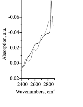
Figure 3: Experimental curve (curve 3 of Fig. 1, the asteric denotes the Nujol absorption band) and the curve calculated by expression (30), or more exactly by formula $K_{||}=C\times[(\omega-2900)^{2}+300^{2}]^{-1}+\frac{1}{800}\sum_{j=0}^{51}[(\omega-120\times(0.5+j))^{2}+(12+0.8j)^{2}]^{-1}$ (dashed line).

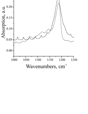
Figure 4: Experimental curve (curve 5 of Fig. 2, solid line) and the curve calculated by expression (30), or more exactly by formula $K_{\perp}=[(\omega-1185)^{2}+20^{2}]^{-1}+\frac{1}{800}\sum_{j=0}^{51}[(\omega-24.5\times(0.5+j))^{2}+(0.1+0.08j)^{2}]^{-1}$ (dashed line).

We can check on solution (27) because the same value of $\mathcal{N}$ should follow from the comparison of the difference between absorption frequencies $\Delta{\kern 1.0pt}\omega_{\ell}$ of two nearest submaximums written, on the one hand, for incident photons and, on the other hand, for excited inerton excitations. In fact, as it is evident from Figs. 1 and 2,

$$\Delta{\kern 1.0pt}\omega_{||}{\kern 1.0pt}=120\,\,{\kern 1.0pt}{\kern 1.0pt}{\rm cm}^{-1}\times{\kern 1.0pt}{\kern 1.0pt}{\kern 1.0pt}c{\kern 1.0pt};\quad\quad\quad{\kern 1.0pt}\,\,\,\Delta{\kern 1.0pt}\omega_{\bot}=24.5\,\,\,{\rm cm}^{-1}\times{\kern 1.0pt}{\kern 1.0pt}{\kern 1.0pt}c$$ (31)

where c is the velocity of light. At the same time, it is evident from the dispersion law (31) that these values also come out to

$$\Delta{\kern 1.0pt}\omega_{\ell}=v_{\ell}{\kern 2.0pt}\Delta q$$ (32)

where allowance is made for the explicit form of the wavenumber $q_{j}$ in the cluster (i.e. $\Delta q=2{\kern 1.0pt}\pi/g{\cal N}$). Substituting values of $\Delta{\kern 1.0pt}\omega_{\ell}$ from expressions (31) into Eq. (32), choosing the corresponding fitting values of the sound velocities $v_{{\kern 0.5pt}||}=4.5\times 10^{{\kern 1.0pt}3}$ m/s and $v_{{\kern 0.5pt}\bot}=1.8\times 10^{3}$ m/s, and setting the crystallite constant $g=3\times 10^{-10}$ m, we will arrive at the same value of hydrogen atoms in a cluster that expression (27) prescribes, $\mathcal{N}=52$.

5. Concluding Remarks

Thus, the IR spectroscopic study of the $\delta$-KIO${}_{3}\cdot$HIO₃ crystal [1] exhibited the band fine structures in the stretching and bending vibrations of hydrogen bonds. The appearance of those substructures has been associated with excited states of hydrogen atoms in clusters, which are formed due to the mechanism stated above. Hydrogen atoms, which enter a cluster, do not move from their equilibrium positions in the crystal backbone, however, the interaction of the hydrogen atoms through the electromagnetic field and the quantum mechanical (i.e. inerton) field brings into existence their synchronous vibrations. Thereby, a fundamentally new type of the interaction between hydrogen atoms, which result in their collective oscillations, has been revealed. Since inertons are carriers of mass, we may say that the atomic mass of hydrogen atoms undergoes periodical oscillations in clusters. The described experiment is of infrequent occurrence, though it has already been known previously: Podkletnov’s phenomenon [31,32], i.e. loss of a part of the mass of electrons in the superconductor state at special conditions, serves as a good example of soundness of the theory proposed.

The estimated number of hydrogen atoms ${\kern 1.0pt}\mathcal{N}=52$ correlates well with the appropriate number calculated from the consideration of the band fine structures.

The phenomenon studied in the present work in fact has demonstrated the inner nature of the interaction of simplest entities, i.e. hydrogen atoms, in the solid. Since the inerton field concerns the matter construction in general, the results obtained in this work might be very required at the investigation of other difficult problems associated with a subtle analysis of physical processes in condensed media.

References

- [1] B. Engelen, T. Gavrilko, M. Panthofer, G. A. Puchkovska, J. Baran, and H. Ratajczak, Selected papers from the Int. Conf. on Spectroscopy of Molecules and Crystals, ed.: G.A. Puchkovska. Proceed. of SPIE, 4938, 15-20 (2002).
- [2] E. D. Belotsky, and B. I. Lev, Theor. Math. Phys. 60, 120 (1984); in Russian.
- [3] V. Krasnoholovets, and B. Lev., Ukr. Fiz. Zh. 33, 296 (1994); in Ukrainian.
- [4] B. I. Lev, and A. Yu. Zhugaevich, Phys. Rev. E 57, 6460 (1998).
- [5] V. Krasnoholovets, and B. Lev, Cond. Matt. Phys. 6, 67 (2003) (also arXiv.org e-print archive cond-mat/0210131). under consideration (also arXiv.org e-print archive, cond-mat/0210131).
- [6] V. Krasnoholovets, and D. Ivanovsky, Phys. Essays 6, 554 (1993) (also arXiv.org e-print archive, quant-ph/9910023).
- [7] V. Krasnoholovets, Phys. Essays 10, 407 (1997) (also arXiv.org e-print archive quant-ph/9903077).
- [8] V. Krasnoholovets, and V. Byckov, Ind. J. Theor. Phys. 48, 1 (2000) (also quant-ph/0007027).
- [9] V. Krasnoholovets, Ind. J. Theor. Phys. 48, 97 (2000) (also quant-ph/0103110).
- [10] V. Krasnoholovets, Ind. J. Theor. Phys. 49, 1 (2001) (also quant-ph/9906091).
- [11] V. Krasnoholovets, Ind. J. Theor. Phys. 49, 85 (2001) (also quant-ph/9908042).
- [12] V. Krasnoholovets, Spacetime & Substance, 1, 172 (2000) (also quant-ph/0106106); Int. J. Comput. Anticipat. Systems, 11, 164 (2002) (also quant-ph/0109012).
- [13] V. Krasnoholovets, Ann. de la Fond. L. de Broglie, 27, no. 1, 93 (2002) (also quant-ph/0202170).
- [14] B. Engelen, T. Gavrilko, M. Panhöfer, G. Puchkovska, and I. Sekirin, J. Mol. Struct. 523, 163 (2000).
- [15] T. Gavrilko, G. Puchkovska, Yu. Polivanov, and A. Yaremko, Ukr. Fiz. Zh. 30, 29 (1985); in Russian.
- [16] A. Barabash, J. Baran, T. Gavrilko, K. Eshimov, G. Puchkovska, and H. Ratajczak, J. Mol. Struct. 404, 187 (1997).
- [17] F. Fallaux, J. Tomkinson, and J. Penfold, Cem. Phys. 124, 425 (1988).
- [18] F. Fallaux, J. P. Fontaine, M. H. Baron. G. J. Kearly, and J. Tomkinson, Chem. Phys. 176, 249 (1993).
- [19] F. Fallaux, J. P. Fontaine, M. H. Baron. G. J. Kearly, and J. Tomkinson, Biophys. Chem. 53, 155 (1994).
- [20] F. Fillaux, N. Leygue, J. Tomkinson, A. Cousson and W. Paulus, Chem. Phys. 244, 387 (1999).
- [21] F. Fillaux, J. Mol. Struct. 511-512, 35 (1999).
- [22] F. Fillaux, Solid State Ionics 125, 69 (1999).
- [23] T. Horsewill, M. Johnson, and H. P. Trommsdorff, Europhys. News 28, 140 (1997).
- [24] Ch. Rambaud, and H. P. Trommsdorff, Chem. Phys. Lett. 306, 124 (1999).
- [25] S. Bratos, and H. Ratajczak, J. Chem. Phys. 76, 77 (1982).
- [26] H. Ratajczak, and A. M. Yaremko, Chem. Phys. Lett. 243, 348 (1995).
- [27] V. G. Vaks, Introduction to the microscopic theory of ferroelectrics (Nauka, Moscow, 1973); in Russian.
- [28] R. Blinc, and B. Žecš, Soft mode in ferroelectrics and antiferroelectrics (North-Holland Publishing Company - Amsterdam, Oxford; American Elsevier Publishing Company, Inc. - New York, 1974).
- [29] V. Krasnoholovets, hep-th/0205196.
- [30] A. S. Davydov, The theory of solid (Nauka, Moscow, 1976); in Russian.
- [31] E. Podkletnov, cond-mat/9701074.
- [32] E. Podkletnov and G. Modanese, physics/0108005.