Quenched bond dilution in two-dimensional Potts models

Abstract

We report a numerical study of the bond-diluted 2-dimensional Potts model using transfer matrix calculations. For different numbers of states per spin, we show that the critical exponents at the random fixed point are the same as in self-dual random-bond cases. In addition, we determine the multifractal spectrum associated with the scaling dimensions of the moments of the spin-spin correlation function in the cylinder geometry. We show that the behaviour is fully compatible with the one observed in the random bond case, confirming the general picture according to which a unique fixed point decsribes the critical properties of different classes of disorder: dilution, self-dual binary random-bond, self-dual continuous random bond.

1 Survey of theoretical and experimental results in $2D$

Quenched disorder coupled to the energy-density has been the subject of an intensive activity in statistical physics, essentially in two-dimensional ($2D$) systems, during the past decades. The qualitative influence of disorder at second order phase transitions is well understood since Harris proposed a celebrated relevance criterion [1]. At first order transitions, randomness obviously softens the transitions, and, under some circumstances may even induce second order transitions according to a picture first proposed by Imry and Wortis [2] and then stated on more rigorous grounds by Aizenman and Wehr [3, 4], implying an important result that an infinitesimal disorder induces continuous transitions in $2D$. The $q-$state Potts model [5] is the natural candidate for the investigations of influence of disorder in a perspective linked to critical phenomena, since the pure model exhibits two different regimes: a second order phase transition when $q\leq 4$ and a first order one for $q>4$ (in $2D$). Many results were obtained in both regimes for self-dual quenched randomness in this model in the last ten years, including perturbative expansions [6, 7, 8, 9, 10, 11, 12, 13], Monte Carlo simulations [14, 15, 16, 17, 18] or Transfer Matrix calculations [19, 20, 21, 22, 23, 24], high-temperature series expansions [25, 26] or recently short-time dynamic scaling [27]. The numerical studies showed that many difficulties, like the lack of self averaging [28, 29, 30, 31] or varying effective exponents due to crossover phenomena may occur. Averaging physical quantities over the samples with a poor statistics may thus lead to erroneous determinations of the critical exponents. We also note that the previoulsy mentioned studies were reported in the case of the random bond system with self-dual probability distributions of the coupling strengths in order to preserve the exact knowledge of the transition line.

In real experiments on the other hand, disorder is inherent to the working-out process and may result e.g. from the presence of impurities or vacancies in a sample produced in Molecular Beam Epitaxy or sputtering experiments. For the description of such a disordered system, dilution is thus more realistic than for example a random distribution of non-vanishing couplings. Since universality is expected to hold in non frustrated random systems, the detailed structure of the Hamiltonian should not play any determining role in universal quantities like critical exponents, but dilution presumably produces a quite strong disorder compared to e.g. a binary random-bond distribution of coupling strengths, and crossover phenomena may alter the determination of the universality class.

Experimentally, the role of disorder in $2D$ systems has been investigated in several systems. Illustrating the influence of random defects in the case of the $2D$ Ising model universality class, samples made of thin magnetic amorphous layers of (Tb_0.27Dy_0.73)_0.32Fe_0.68 of 10 Å  width, separated by non magnetic spacers of 100 Å  Nb in order to decouple the magnetic layers were produced using sputtering techniques. A structural analysis (high resolution transmission electron microscopy and $x$-ray analysis) was performed to characterize the defects inherent to such amorphous structures (types of voids or possibly compositional disorder), and in spite of these random defects separated on average by a distance of a few nm, the samples were shown to exhibit Ising-like singularities with critical exponents $\beta=0.126(20)$, $\gamma=1.75(3)$ and $\delta=15.1(10)$ [32]. This is coherent with the fact that disorder does not change the universality class of the $2D$ Ising model, apart from logarithmic corrections which are not easy to observe experimentally, since their role becomes prominant only in the very neighbourhood of the critical point. For this reason, the Ising model is probably not the best system to study quantitatively the influence of randomness experimentally.

More interesting from the point of view of critical phenomena is the case of a beautiful experimental confirmation of the Harris criterion reported in a Low Energy Electron Diffraction (LEED) investigation of a $2D$ order disorder transition [33] belonging to the 4-state Potts model universality class. Order-disorder transitions of adsorbed atomic layers are known to belong to different two-dimensional universality classes depending on the type of superstructures in the ordered phase of the adlayer [34, 35]. The substrate plays a major role in adatom ordering, as well as the coverage (defined as the number of adatoms per surface atom) which determines the possible superstructures of the overlayer. For example, sulfur chemisorbed on Ru$(001)$ exhibits four-state or three-state Potts critical singularities for the $p(2\times 2)$ and the $(\sqrt{3}\times\sqrt{3})R30^{\circ}$ respectively [36] (at coverages $1/4$ and $1/2$). Other examples can be found in the literature, for example oxygen on Ru$(0001)$ ordered in a $p(2\times 2)$ [37] or $p(2\times 2)$-Cs or K on Cu$(111)$ [38] also belong to the four-state Potts universality class, while $(\sqrt{3}\times\sqrt{3})R30^{\circ}-1$CO has three-state Potts singularities [39]. The case of the $(2\times 2)-$2H/Ni$(111)$ order-disorder transition of hydrogen adsorbed on the $(111)$ surface of Ni thus belongs to the $2D$ four-state Potts model universality class (with expected exponents $\beta=1/12\simeq 0.083$, $\gamma=7/6\simeq 1.167$, and $\nu=2/3\simeq 0.667$ for example).

Using LEED, it is possible to measure these exponents through the diffracted intensity $I({\bf q})$ or structure factor. This is the two-dimensional Fourier transform of the pair correlation function of adatom density, where long range fluctuations produce an isotropic Lorentzian centered at the superstructure spot position ${\bf q}_{0}$ with a peak intensity given by the susceptibility and a width determined by the inverse correlation length, while long range order gives a background proportional to the order parameter squared:

$$I({\bf q})=\langle m^{2}\rangle\delta({\bf q}-{\bf q}_{0})+\frac{\chi}{1+\xi^{2}({\bf q}-{\bf q}_{0})^{2}}.$$ (1)

The following exponents were thus measured [33, 40, 41] $\beta=0.11\pm 0.01$, $\gamma=1.2\pm 0.1$ and $\nu=0.68\pm 0.05$ in correct agreement with 4-state Potts values (the small deviation, especially for the exponent $\beta$, is possibly attributed to the logarithmic corrections to scaling of the pure 4-state Potts model [42]). The same experiments were then reproduced in the presence of intentionally added oxygen impurities, at a temperature which is above the ordering temperature of pure oxygen adsorbed on the same substrate. The mobility of these oxygen atoms is furthermore considered to be low enough at the hydrogen order-disorder transition critical temperature that they essentially represent quenched impurities randomly distributed in the hydrogen layer, and the new measured exponents become $\beta=0.135\pm 0.010$, $\gamma=1.68\pm 0.15$ and $\nu=1.03\pm 0.08$. It definitely rules out the role of these oxygen impurities as extended defects, like steps for example, which, according to Ref. [33], produce a rounding of the transition by a simple finite-size-scaling effect. The modification of the universality class in the presence of quenched disorder is understood with Harris criterion which predicts such a situation when the exponent $\alpha$ of the specific heat is positive for the pure system ($\alpha=2/3$ for the 4-state Potts model).

The aim of this paper is to perform numerical simulations of the bond diluted Potts model for several values of the number of states per spin (in order to cover the two different regimes of the pure system’s phase transitions) and provide a reliable comparison of the diluted and random-bond problems. This will be achieved through a systematic comparison with previous results obtained for self-dual random-bond disorder. Here we stress that self-duality is an internal symmetry which can lead to some simplifications that the dilute problem does not present and thus it is worth comparing both problems. In section 2, the details of the numerical techniques are summarized. This section also provides an exposition of the different extrapolation techniques in order to leave the discussion of the physical results to the following of the paper. Section 3 presents the phase diagram of the diluted Potts models with $q=3$, 4, and 8, and section 4 the results of transfer matrix calculations and the critical behaviour of the order parameter correlation function.

2 Methodology and numerical techniques

2.1 Definition of the model

In this paper, we study the 2-dimensional diluted $q$-state Potts model defined by the following Hamiltonian :

$$-\beta{\cal H}=\sum_{(i,j)}K_{ij}\delta_{\sigma_{i},\sigma_{j}}$$ (2)

where the sum is restricted to nearest neighbours on a square lattice, the degrees of freedom $\{\sigma_{i}\}$ can take $q$ values and the exchange couplings $\{K_{ij}\}$ are quenched independent random variables chosen according to a binary distribution of non vanishing and vanishing values

$${P}(K_{ij})=p\ \!\delta(K_{ij}-K)+(1-p)\delta(K_{ij}).$$ (3)

The value $p=1$ corresponds to the pure system and $p_{c}=1/2$ is the bond percolation threshold. Below this threshold there cannot exist any ordered state at finite temperature and the phase transition temperature vanishes.

2.2 Transfer matrix study

The system is first studied using the transfer matrix method introduced by Blöte and Nightingale [43], which takes advantage of the Fortuin-Kasteleyn representation [44] in terms of graphs of the partition function of the Potts model in order to reduce the dimension of the Hilbert space. In the Fortuin-Kasteleyn representation, the transfer matrix (with no magnetic field)

$$Z={\rm Tr}\prod_{(i,j)}(1+\delta_{\sigma_{i},\sigma_{j}}u_{ij}),$$ (4)

where $u_{ij}={\rm e}^{K_{ij}}-1$, is expanded as a sum over all the possible graphs $g$ (with $s$ sites, $l(g)$ loops and $c(g)$ independent clusters) leading to the random cluster model:

$$Z=q^{s}\sum_{g}q^{l(g)}\prod_{(i,j)/b_{ij}=1}\left(\frac{u_{ij}}{q}\right),$$ (5)

$b_{ij}$ being the bond variables. Blöte and Nightingale suggested to introduce a set of connectivity states which contain the information about which sites on a given row belong to the same cluster when they are interconnected through a part of the lattice previously built. A unique connectivity label $\eta_{i}=\eta$ is attributed to all the sites $i$ of such a cluster. In the connectivity space, $|Z(m)\rangle$ is a vector whose components are given by the partial partition function $Z(m,\{\eta_{i}\}_{m})$ of a strip of length $m$ whose connectivity on the last row is given by $\{\eta_{i}\}_{m}$. The connectivity transfer matrix is then defined according to $|Z(m+1)\rangle={\bf T}_{m}|Z(m)\rangle$ and the partition function of a strip of length $m$ becomes $|Z(m)\rangle=\prod_{k=1}^{m-1}{\bf T}_{k}|Z(1)\rangle$, where $|Z(1)\rangle$ is the statistics of uncorrelated spins.

2.2.1 Free Energy Density

The quenched free energy density is given by the Lyapunov exponent of the product of an infinite number of transfer matrices ${\bf T}_{k}$ [45]

$$\overline{f_{L}}=-L^{-1}\Lambda_{0}(L).$$ (6)

$$\Lambda_{0}(L)=\lim_{m\to\infty}\frac{1}{m}\ln\left|\!\left|\left(\prod_{k=1}^{m}{\bf T}_{k}\right)\mid\!v_{0}\rangle\right|\!\right|,$$ (7)

where $\mid\!v_{0}\rangle$ is a unit initial vector. In order to determine the error induced by the truncation of this product to a finite number of terms, we studied the fluctuations of the free energy density with respect to the number of iterations of the transfer matrix. The tests have only been performed for the 4-state Potts model on strips of width $L=8$ with a pseudo critical exchange coupling $K_{c}=1.16215$ at the dilution $p=0.75$. This value of the exchange coupling is a rough estimate of the critical exchange coupling at this dilution as it will be shown later.

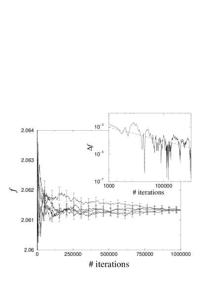
Figure 1: Convergence of the free energy density (for five different disorder realisations) as a function of the number of iterations of the transfer matrix. For the sake of clarity, error bars are only displayed every 50000 iterations. The parameters take the following values $L=8$, $p=0.75$, $K_{c}=1.16215$. The inset shows statistical fluctuations $\Delta f=\sqrt{\overline{f^{2}}-\bar{f}^{2}}$ of free energy density with respect to the number of iterations. The dashed line (which is a guide for the eyes) is a power-law with exponent $-1/2$.

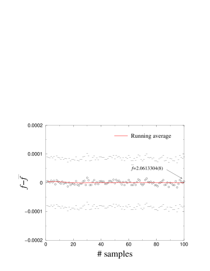
Figure 2: Convergence of the average of the free energy density $f$ obtained by iterating $10^{6}$ times the transfer matrix with respect to the number of disorder realisations entering the average. Each circle corresponds to the free energy density of a given sample and the dots to the upper and lower bounds of its error bar. The solid line is the running average and the final estimate $\langle f\rangle$ is written at its right edge. The parameters take the following values $L=8$, $p=0.75$, $K_{c}=1.16215$.

In figure 1, we present the estimates of the free energy density for five independent runs and the inset shows its standard deviation. For a self-averaging quantity $X$, the reduced standard deviation squared should be proportional to the inverse volume of the system, $R_{X}=(\overline{X^{2}}-\bar{X}^{2})/\bar{X}^{2}\sim 1/LN$ (the number of iterations $N$ of the transfer matrix is the length of the strip), and thus at fixed strip width $L$, $\Delta X\sim 1/\sqrt{N}$. The standard deviation of the free energy density indeed exhibits an inverse square root decay $1/\sqrt{N}$ with the number $N$ of iterations of the transfer matrix (see inset in figure 1), i.e. it reveals that the estimates of the free energy density are weakly correlated from row to row and the free energy is self-averaging. It thus turns out to be preferable to average the estimates of the free energy density obtained by different runs rather than using very long strips for which one would accumulate truncation errors. Figure 2 shows such an example of average of the free energy density estimated by independent runs. Despite the fact that the standard deviation of the free energy density seems to over-estimate the true error by at least one order of magnitude, this definition of the error is a safe choice and will be kept in the following. Up to now, all runs have been performed using $100$ independent runs of $10^{6}$ iterations of the transfer matrix, leading to an accuracy of 6-7 digits in the free energy density.

2.2.2 Central charge

For a pure system, the central charge $c$ is defined as the universal coefficient in the lowest-order correction to scaling of the free energy density ${f_{L}}$:

$${f_{L}}=f_{\infty}-L^{-2}\left[{\pi c\over 6}\right. +b_{\omega}L^{-\omega}+b_{2\omega}L^{-2\omega}+\dots$$ (8)

$$\left.+a_{2}L^{-2}+a_{4}L^{-4}+\dots\phantom{a\over b}\right],$$

where the regular contribution is

$$f_{\infty}=\lim_{L\rightarrow+\infty}{f_{L}}$$ (9)

and $-\omega$ is the exponent associated to the irrelevant vacancy field [46, 47, 48, 49]. For a disordered system, $c$ is defined in the same way from the finite-size behaviour of the quenched average free energy density $\overline{f_{L}}$, and numerically, since the strip widths available are small, we can only expect to measure effective central charges which depend on the dilution, $c_{eff}(p)$, and which would converge towards the true value $c$ in the thermodynamic limit. One obviously expects the existence of higher order corrections to scaling, but since no analytical expression is known, we cannot include explicite size dependence for higher order terms and the possible corrections are taken into account by fitting the free energy density including a $1/L^{4}$ non universal correction [50, 51]

$$\overline{f_{L}}=f_{0}-{\pi c_{eff}\over 6L^{2}}+a_{2}L^{-4}.$$ (10)

Fits with polynomials in $1/L^{2}$ of degrees ranging from 2 to 4 (i.e. up to $L^{-8}$) were also considered, but do not increase the accuracy.

2.2.3 Improvement of the calculation of the central charge

In order to obtain more accurate estimates of the critical temperature, especially at small values of the number of states $q$ where the slow variation of the effective central charge makes this determination difficult, we have used a semi-analytical transfer matrix. Instead of computing the product of the transfer matrices at a given value of the parameter $u=e^{K}-1$, the calculations are performed at $u+\delta u$. All elements of the transfer matrices are expressed as polynomials of $\delta u$. This parameter shift $\delta u$ is supposed small and the polynomials are truncated to the second order in $\delta u$. The free energy and its error bar are thus expressed as polynomials of $\delta u$ too and can be numerically computed over a continuous range of parameters centered around $u$. The central charge is then extrapolated using the fitting procedure previously presented. An example of such a calculation is given by the figure 3, where the solid lines show the central charge (with up and down limits of the error bars) as a continuous function of $K$, compared to a set of independent computations (circles) at fixed coupling strengths.

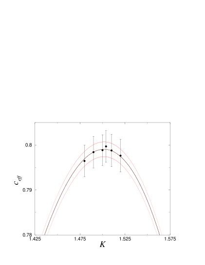
Figure 3: Central charge $c_{eff}$ of the 3-state Potts model at dilution $p=0.75$ versus the exchange coupling $K$ as obtained with independent runs of 100 samples (symbols) and with a semi-analytic calculation with 500 samples of $10^{6}$ iterations of the transfer matrix (solid curve). The ditted lines correspond to the up and down limits of the errors bars of the semi-analytic calculation.

2.2.4 Phase diagram

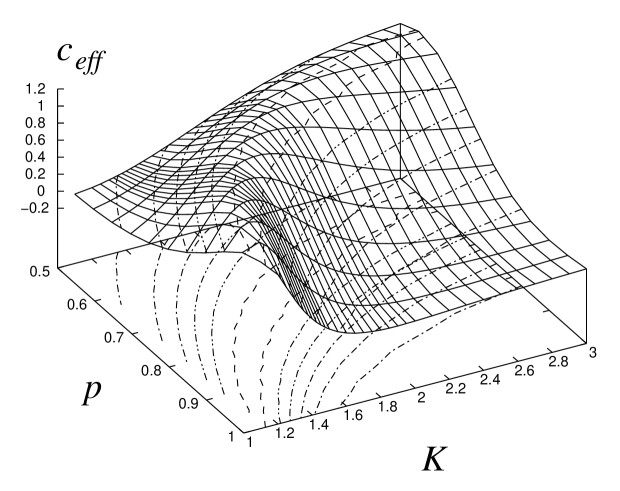
Figure 4: Dependence of the effective central charge $c_{eff}$ with the exchange coupling $K$ and the bond probability $p$ for the 4-state Potts model. The maximum of $c_{eff}$ gives the location of the transition line.

The phase diagram can be obtained as usually by the evolution of the maximum of some diverging quantity, let say the susceptibility for example which diverges at criticality in the thermodynamic limit. In the strip geometry considered here, we preferred another technique based on the behaviour of the effective central charge. In usual critical systems, the Zamolodchikov’s $c-$theorem states that there exists a $c-$function decreasing along RG flows and giving the central charge at the fixed point [52]. In the case of random systems ($n\to 0$ in the replica approach), the central charge increases and can be expected to reach a maximum value at an optimal disorder amplitude. This property, linked to non-unitarity in the presence of disorder, is indeed observed in simulations [22, 16, 23, 24, 50, 51]. This property is illustrated in figure 4 where we can follow the maximum of the effective central charge in the plane $(p-K)$.

2.2.5 Correlation Functions

The spin-spin correlation functions along the strip are calculated using an extension of the Hilbert space that allows to keep track of the connectivity with a given spin. For a specific disorder realisation, the spin-spin correlation function along the strip

$$G_{\sigma}(\tau)=\frac{q\langle\delta_{\sigma_{j}\sigma_{j+\tau}}\rangle-1}{q-1},$$ (11)

where $\langle\dots\rangle$ denotes the thermal average, is given by the probability that the spins along some row, at columns $j$ and $j+\tau$, are in the same state and is expressed in terms of a product of the non-commuting transfer matrices:

$$\langle\delta_{\sigma_{j}\sigma_{j+\tau}}\rangle=\frac{\langle 0\!\mid{\bf g}_{j}\left(\prod_{k=j}^{j+\tau-1}{\bf T}^{\prime}_{k}\right){\bf d}_{j+\tau}\mid\!0\rangle}{\langle 0\!\mid\prod_{k=j}^{j+\tau-1}{\bf T}_{k}\mid\!0\rangle},$$ (12)

where $\mid\!0\rangle$ is the ground state eigenvector, ${\bf T}_{k}^{\prime}$ is the transfer matrix in the extended Hilbert space. The operator ${\bf g}_{j}$ identifies the cluster containing $\sigma_{j}$, while ${\bf d}_{j+\tau}$ gives the appropriate weight depending on whether or not $\sigma_{j+\tau}$ is in the same state as $\sigma_{j}$. They were computed on strips of widths $L=2$ to 8 and then averaged over $100\ 000$ disorder realisations.

Figure 5: Histograms of probability distributions of the spin-spin correlation function at given distances $\tau=100$, 75, 50 and 25 (from left to right) for the 4-state Potts model with an exchange coupling $K=1.16215$ and at dilution $p=0.75$. Note that the scale is logarithmic on the $x$-axis.

The numerical calculation of the average over randomness of these spin-spin correlation functions is made difficult by the fact that they are not self-averaging. Indeed, Figure 5 shows that the probability distribution is close to a log-normal distribution (the correlation function is given by a product of matrices whose elements are reminiscent of randomness). There are thus some rare events $G_{\sigma}(\tau)\sim{\cal O}(1)$ with a large relative contribution to the average. This is especially true at large distances. An accurate estimation of the average requires that the sampling includes such events. As can be seen in figure 6, the running average of the spin-spin correlation function presents jumps due to these rare events. The error bars are underestimated as the standard deviation of the correlation functions (which cannot correspond to the true definition of the error on data distributed according to a clearly non Gaussian distribution).

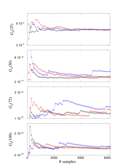
Figure 6: Convergence of the spin-spin correlation functions $G_{\sigma}(\tau)$ at a given distance $\tau=100$, 75, 50 and 25 (from bottom to top) with respect to the number of disorder realisations (up to 6200 samples).

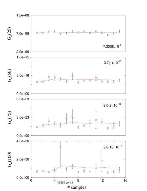
Figure 7: Convergence of the average of the spin-spin correlation functions $G_{\sigma}(\tau)$ at a given distance $\tau$ with respect to the number of bins of $6200$ disorder realisations.

In the following, results are obtained using an average over 100000 disorder realisations. As shown in figure 7, it seems that the rare events have been sufficiently well sampled with this number of disorder realisations, since the running average remains flat and no systematic deviation is seen. For some disorder realisations, there can be one or several rows with no bond at all. Such cuts disconnect the strip in two subsystems and the correlation function is thus vanishing for larger distances for the corresponding realisations, inducing a discontinuity of $G_{\sigma}(\tau)$. The average being performed over a finite number of disorder realisations, these cuts lead to jumps in the average correlation functions (figure 8). These jumps are more pronounced for moments $\overline{G^{n}(\tau)}$ of increasing order $n$ because the contribution of the rare events is enhanced and the average is determined by a few configurations that can include such jumps. The averaged moments are also less fluctuating (with the distance) for larger strip widths.

Figure 8: Jumps in the $4^{\rm th}$-moment of the spin-spin correlation functions with respect to the distance at $q=4$, $p=0.70$ and $K=0.81$. The different curves correspond to lattice sizes ranging from $2$ to $8$ and the average is performed over 100 000 samples. The power $L$ ensures the same asymptotic slope for different strip widths.

2.3 Methodology used in the computations

For each value of the number of states, $q$, a few runs are performed with $100\times 10^{6}$ iterations in order to have at each strip width an evaluation of the free energy density $\overline{f}(K,p)$. Then, after extrapolation at $L\to\infty$, the effective central charge $c_{eff}(K,p)$ is evaluated in the temperature-dilution plane. This leads to a first approximate determination of the phase diagram $K_{c}(p)$. For each dilution $p$, new runs are performed with the semi-analytical algorithm (see section 2.2.3) at $K_{max}$, the coupling strength corresponding to the maximum of $c_{eff}$. A total of $500\times 10^{6}$ iterations of the transfer matrix are thus used. When the curve $c_{eff}(p)$ is very flat, the computation is done for two distinct values of $p$. The spin-spin correlation functions are then computed at the maximum of $c_{eff}(p)$ with $500\ 000$ configurations.

3 Phase diagram of the diluted $q$-state Potts model

According to the previous section, the phase diagrams of diluted Potts models with $q=3$, $4$ and $8$ states per spin are first determined by the location of the maxima of the central charge in strip geometries in the $(p,K)$ plane. The effective central charge is shown in figure 9 for several dilutions, as a function of $K$.

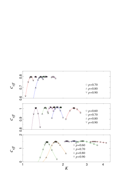
Figure 9: Estimation of the central charge with respect to the exchange coupling for several dilutions (for $q=3$ (top), $q=4$ (middle) and $q=8$ (bottom)).

Figure 10: Phase diagram of the $q$-state diluted Potts model obtained numerically (symbols) and compared with the single-bond effective medium approximation (solid lines). The open circles on each critical line give the loci of the optimal dilutions which will be discussed later.

The phase diagrams of quenched bond disordered Ising and Potts models were studied more than twenty years ago using effective-medium approximation [54, 55]. The Hamiltonian is written

$$-\beta{\cal H}=\sum_{(i,j)}K_{m}\delta_{\sigma_{i},\sigma_{j}}+\sum_{(i,j)}x_{ij}\delta_{\sigma_{i},\sigma_{j}}$$ (13)

where $x_{ij}=K_{ij}-K_{m}$ is the deviation from the effective medium homogeneous coupling strength. Using the identity ${\rm e}^{x_{ij}\delta_{\sigma_{i},\sigma_{j}}}=1+\delta_{\sigma_{i},\sigma_{j}}({\rm e}^{x_{ij}}-1)$, one gets a formal exact expression for the thermal average of any quantity $Q$ as

$$\langle Q\rangle=\frac{\langle Q\prod_{(i,j)}[1+\delta_{\sigma_{i}\sigma_{j}}({\rm e}^{x_{ij}}-1)]\rangle_{m}}{\langle\prod_{(i,j)}[1+\delta_{\sigma_{i}\sigma_{j}}({\rm e}^{x_{ij}}-1)]\rangle_{m}}$$ (14)

where $\langle\dots\rangle_{m}$ stands for the average with Boltzmann factors ${\rm e}^{-\beta{\cal H}_{m}}$ with

$$-\beta{\cal H}_{m}=\sum_{(i,j)}K_{m}\delta_{\sigma_{i},\sigma_{j}}.$$ (15)

A single bond approximation ($x_{ij}=0$ everywhere except on one particular bond) then leads to the equation of the critical line

$$K_{c}(p)=\ln\frac{(1-p_{c}){\rm e}^{K_{c}}-(1-p)}{p-p_{c}}.$$ (16)

This expression should be exact in the vicinity of both the pure system and the percolation threshold. Inserting the critical coupling for the pure system $K_{c}=\ln(1+\sqrt{q})\equiv K_{c}(p=1)$ and the percolation threshold $p_{c}=1/2$ of bond percolation on the square lattice indeed leads to an excellent agreement with the numerical data (see figure 10). We also note that the approximation has been improved by a cluster extension of the effective interaction [56].

4 Critical behaviour

4.1 Critical behaviour of spin-spin correlation functions

If the assumption of the existence of a unique stable random fixed point holds, one expects that the critical behaviour is asymptotically the same as the system is moved along the transition line $p_{c}<p<1$. However, in finite systems, one generically has to deal with strong crossover effects due to the competition between the disordered fixed point and the pure (at $p=1$) and percolation (at $p=p_{c}$) fixed points, or to corrections to scaling linked to the appearence of irrelevant scaling variables. It is known that these latter effects are generally important in random systems and that the corresponding corrections to scaling can be substantially reduced when one measures the critical exponents in the regime of the random fixed point, expected to be reached at the vicinity of the maximum of the effective central charge in the $p$-direction (as shown below). Let us consider the finite-size behaviour of an observable $Q$ measured at a deviation $t=K-K_{c}(p)$ from the critical point on some system of characteristic size $L$, in the presence of dilution at bond probability $p$. The variables $t$ and $L^{-1}$ play the role of relevant scaling fields (with positive RG eigenvalues $y_{t}=1/\nu$ and $y_{L}=1$ respectively), while close to the fixed point, dilution is supposed to be related to some irrelevant scaling variable with eigenvalue $y_{p}=-\omega<0$. At the fixed point there is no need that the irrelevant scaling field vanishes, so that one can write $p^{*}$ the corresponding dilution and the observable $Q$ obeys the following homogeneity assumption in the scaling region

$$Q(t,L^{-1},p)=L^{-x_{Q}}f(L^{1/\nu}t,L^{-\omega}(p-p^{*}))$$ (17)

which corresponds to the same critical behaviour for any value of $p$ in the range $p_{c}<p<1$, described by a unique fixed point. An expansion of the last variable (keeping the leading term only) along the critical line (i.e. varying $p$ at $K_{c}(p)$) gives

$$Q(0,L^{-1},p)=\Gamma_{Q}L^{-x_{Q}}(1+\Gamma_{Q}^{(2)}(p-p^{*})L^{-\omega}+\dots),$$ (18)

where the $\Gamma_{Q}$’s are non-universal critical amplitudes. It is thus possible to fix $p=p^{*}$ in order to minimize the corrections to scaling, and the corresponding value of the dilution is empirically found to coincide with the location of the maximum of the central charge along the critical line [23]. Close to the maximum, the variations of the effective central charge itself are small, illustrating that corrections to scaling have there a small influence which is consistent with our choice in equation (10). The value of $p^{*}$ is not universal and should depend on the system shape, boundary conditions, etc.

In figure 11, we show the variation of the effective central charge along the transition line. For example in the case $q=4$, the random fixed point corresponds roughly to the optimum dilution $p^{*}\sim 0.700$. The estimate of the central charge at this random fixed point is $c^{*}=1.0148(40)$ which is less accurate but perfectly compatible with the one obtained in the random-bond case with a binary distribution of coupling strengths ($c^{*}=1.0148(4)$) . This value has been refined using the semi-analytical transfer matrix presented before and a 5-time larger statistic, leading to $c^{*}=1.0143(19)$ at $K_{c}^{*}=1.8072$. Here and in the following, a star superscript is used to mark the values of the parameters which lead to the maximum of $c_{eff}(K,p)$.

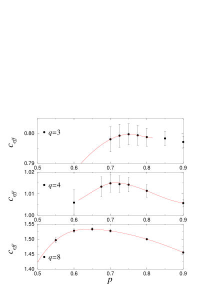
Figure 11: Estimation of the dilution $p^{*}$, where the central charge takes its maximum value. The data points correspond to computations performed at different temperatures, along the critical line, determined by the value of the probability $p$. The solid lines are simple guides for the eyes.

Once the optimal values $K_{c}^{*}$ and $p^{*}$ are located, we compute the correlation functions at the corresponding point in the parameter space. An effective magnetic critical exponent $x_{\sigma}(L)$ for a given strip width $L$ is obtained by fitting the average spin-spin correlation functions with the ansatz

$$\overline{G_{\sigma}(\tau)}={A}\exp\left(-\frac{2\pi}{L}x_{\sigma}(L)\tau\right)$$ (19)

deduced from the logarithmic conformal transformation which maps the infinite plane onto an infinitely long cylinder. Here, $\tau$ is the coordinate along the cylinder (strip with periodic boundary conditions in one direction). Conformal mappings of average profiles and correlation functions were shown to allow accurate determination of the critical exponents in disordered systems, at least in the case of the random-bond Potts model [23], and we naturally assume here that such transformations also apply in the diluted problem.

The data for $q=3$, 4, and 8 are summarized in table 1, where our best estimate is written in bold face. We can notice that although the critical exponents of the diluted and random-bond systems are quite close as expected, the rather small error bars are probably underestimated, and may not reflect the true deviation when it is due to insufficient disorder average.

The $L$-dependence of the magnetic critical exponent is due to corrections to scaling (due for example to the above-mentioned crossover effects) which are not explicitly taken into account in (19). These effective magnetic critical exponents $x_{\sigma}(L)$ are then extrapolated in the limit $L\rightarrow+\infty$ using a polynomial of degree $2$ in $1/L$. Strip widths between $3$ and $8$ have been used. The critical exponent associated to the decay of the average spin-spin correlation function is for example estimated to be $x_{\sigma}\simeq 0.1419(1)$ in the case $q=4$. This estimate is above (but outside error bars) the estimate obtained for the 4-state Potts model in the random-bond case ($0.1385(3)$) in the regime of the random fixed point. We also note that a very close value is obtained at the critical temperature for the dilution $p=0.725$ ($x_{\sigma}=0.1412(1)$).

In the case $q=8$, we obviously expect the first-order phase transition of the pure 8-state Potts model to be turned into a second order one under the influence of randomness [3]. We indeed observed an exponential decay of the spin-spin correlation functions in the longitudinal direction of the strip with a correlation length diverging with $L$, which supports this hypothesis. The phase-diagram is qualitatively the same as in the case of the 4-state Potts model. The regime of the random fixed point corresponds in this case to the dilution $p^{*}\simeq 0.65$. For the random-bond Potts model, the central charge in the regime of the random fixed point was $c^{*}=1.5300(5)$ which is roughly what is obtained in the diluted case at the maximum of the central charge $c^{*}=1.5320(23)$ at dilution $p^{*}=0.650$ (figure 11). A calculation using the semi-analytical transfer matrix yields the estimate $K_{c}^{*}=2.40420$ for the critical exchange coupling. Unfortunately, the calculation of the spin-spin correlation functions is made difficult by the large weight of rare events leading to decays of correlation functions presenting jumps when the number of disorder realisations is too small (as already mentioned at the end of section 2). Using 500,000 disorder realisations, the decay of the average correlation functions yields the critical exponent $x_{\sigma}=0.1514(2)$ which is close, although again outside error bars, to the estimate in the random-bond case ($0.1505(3)$).

Table 1: Central charge and magnetic critical exponent of the $q-$state diluted Potts model compared to the random bond Potts model at the corresponding random fixed point.

• 	Diluted systems
  $q$	$p$	$K_{c}$	$c$	$x_{\sigma}$	$\#$ of samples
  3	0.750	1.5004	0.800(4)		$100\times 10^{6}$
  	0.775	1.4300	0.799(3)		$100\times 10^{6}$
  	0.750	1.50165	0.799(2)	0.13495(6)	$500\times 10^{6}$
  	0.775	1.42740	0.799(2)	0.13522(6)	$500\times 10^{6}$
  4	0.700	1.8100	1.0148(40)		$100\times 10^{6}$
  	0.725	1.7120	1.0144(40)		$100\times 10^{6}$
  	0.700	1.8072	1.0143(19)	0.1419(1)	$500\times 10^{6}$
  	0.725	1.7075	1.0140(18)	0.1412(1)	$500\times 10^{6}$
  8	0.650	2.40420	1.5320(23)	0.1514(2)	$500\times 10^{6}$
  	Random Bond systems
  $q$	distribution		$c$	$x_{\sigma}$
  3	binarya		0.7998(4)	0.1347(11)
  	ternarya			0.1344(8)
  	quaternarya			0.1343(6)
  	continuousa			0.1344(13)
  4	binaryb		1.0148(4)	0.1385(3)
  8	binaryb		1.5300(5)	0.1505(3)

• ^a From C. Chatelain and B. Berche, Nucl. Phys. B 572, 626 (2000).

• ^b From C. Chatelain and B. Berche, Phys. Rev. E 60, 3853 (1999).

In the case $q=3$, the procedure is again identical to that of the 4 and 8-state Potts model presented before. The peak of the central charge with respect to the exchange coupling are narrower than for larger values of $q$ (figure 9). This leads to a better defined phase diagram (figure 10) than for $q=4$ and $q=8$. Nevertheless, the error bars on the central charge are of the order of magnitude of its variation with the dilution $p$. It is thus difficult to define precisely its maximum, approximately located at $p^{*}=0.75$. The effective critical exponent, as given by the decay of the spin-spin correlation, depends much more on the precision on the critical exchange coupling $K_{c}^{*}$ than for larger value of $q$. The semi-analytical transfer matrix at the dilution $p=0.75$ with an average of the free energy over $500$ products of $10^{6}$ iterations of the transfer matrix gives the refined estimate $K_{c}^{*}\simeq 1.50165$. The maximum of the central charge is $0.799(2)$ which is compatible, within error bars, with the value $0.7998(4)$ obtained in the random bond case. The estimate of the magnetic critical exponent at this point $0.13495(6)$ is compatible with the value obtained in the random-bond case $0.1347(11)$ and with the estimate $0.13465$ obtained by perturbative developments in the neighborhood of $q=2$.

4.2 Multifractal behaviour of the spin-spin correlation function

In this section, we report a study of the multifractal properties of the spin-spin correlation functions of the diluted Potts model. A similar analysis was performed in the random-bond case in Ref. [24]. The aim is to provide in the diluted case also a test of replica symmetry breaking using the multifractal behaviour of the spin-spin correlation functions, then to compare the multifractal spectrum for different values of $q$.

The critical exponent $x_{\sigma^{2}}$ associated to the algebraic decay of the second moment $\overline{G^{2}_{\sigma}(\tau)}^{1/2}$ of the spin-spin correlation function was calculated using a perturbation expansion around the conformal field theory at $q=2$ with the assumption that replica symmetry holds or is spontaneously broken. At $q=3$, the expansion based on the replica symmetric scenario was shown to be in a very good agreement with the numerical data for the random-bond problem. In the diluted case, we confirm this agreement, as can be seen in table 2.

Table 2: Magnetic critical exponent of the second moment of the spin-spin correlation function of the $3-$state diluted Potts model compared to the random bond Potts model at the corresponding random fixed point. The perturbative results of Dotsenko et al. are recalled.

• Transfer matrix
  Randomness	distribution	$x_{\sigma^{2}}$
  Dilution		0.1184(1)
  Random bond	binary	0.1177(12)a
  	ternary	0.1182(12)a
  	continuous	0.1173(14)a
  Perturbation
  Replica symmetry		0.11761b
  Replica symmetry breaking		0.12011b

• ^a From C. Chatelain and B. Berche, Nucl. Phys. B 572, 626 (2000).

• ^b From Vik. Dotsenko, Vl. Dotsenko and M. Picco, Nucl. Phys. B250, 633 (1998).

More generally, the critical behaviour of the moments of the correlation function is characterized by a set of exponents $x_{\sigma^{n}}$ which depend on the moment order $n$ in the case of multifractality. Numerically, these exponents are obtained by a simple generalization of equation (19) to:

$$\overline{G_{\sigma}^{n}(\tau)}^{1/n}={A_{n}}\exp\left(-\frac{2\pi}{L}x_{\sigma^{n}}(L)\tau\right)$$ (20)

with the extrapolation to $L\to\infty$. The exponents associated to the first integer order moments are given in table 3 and compared to the corresponding random-bond values and to the perturbative results in the replica symmetric scenario [13]. The plot is shown in figure 12.

Table 3: Magnetic critical exponent of the moments of the spin-spin correlation function of the $3-$state diluted Potts model compared to the random bond Potts model at the corresponding random fixed point. The perturbative results of Lewis are recalled (the expansion is only valid for $q$ close to the Ising value $q=2$ and at small moment order $n$ close to 1).

• 	$x_{\sigma^{n}}$
  		Transfer matrix
  $n$	theor.a	binaryb	continuousb	diluted
  1	0.13465	0.1347(11)	0.1344(13)	0.13522(6)
  2	0.11761	0.1177(25)	0.1173(28)	0.11841(11)
  3	0.11006	0.1051(39)	0.1070(45)	0.10552(17)
  4	-	0.0938(50)	0.0996(58)	0.09511(21)
  5	-	0.0822(58)	0.0906(66)	0.08630(25)

• ^a From M.A. Lewis, Europhys. Lett. 43, 189 (1998).

• ^b From C. Chatelain and B. Berche, Nucl. Phys. B 572, 626 (2000).

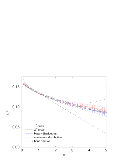
Figure 12: Exponents of the moments of the correlation function, $x_{\sigma^{n}}$ plotted against the moment order for $q=3$. A convincing agreement follows from comparison with 1st and 2nd order expansion calculations and also with numerical results obtained for random-bond models.

An interesting quantity is given by the Legendre transform $H(\alpha)$ of the set of exponents $X_{\sigma^{n}}=nx_{\sigma^{n}}$,

$$H(\alpha)=X_{\sigma^{n}}-n\alpha,\ \alpha={\partial X_{\sigma^{n}}\over\partial n},\ n=-\frac{\partial H}{\partial\alpha}.$$ (21)

This multifractal function is naturally introduced through the probability distribution of the quantity of interest. The exponential decay of the moments of the correlation function along the strip

$$\overline{[G_{\sigma}(\tau)]^{n}}\equiv\int_{0}^{1}[G_{\sigma}(\tau)]^{n}P_{\tau}(G){\rm d}G\sim\exp\left(-\frac{2\pi}{L}X_{\sigma^{n}}(L)\tau\right),$$ (22)

may be seen as a function $L_{\tau}(n)$, which is, by construction, the Laplace transform of the probability distribution $P_{\tau}(y)$ at fixed $\tau$, with the positive variable $y=-\ln G_{\sigma}(\tau)$:

$$\overline{[G_{\sigma}(\tau)]^{n}}\equiv L_{\tau}(n)=\int_{0}^{\infty}{\rm e}^{-ny}P_{\tau}(y){\rm d}y.$$ (23)

Inverting the Laplace transform,

$$P_{\tau}(y)=\frac{1}{2{\rm i}\pi}\int_{\delta-{\rm i}\infty}^{\delta+{\rm i}\infty}{\rm e}^{-\frac{2\pi\tau}{L}[X_{\sigma^{n}}-ny/(2\pi\tau/L)]}{\rm d}n$$ (24)

and performing a saddle-point approximation of the Bromwich integral [57], a similar exponential expression follows for the probability distribution

$$P_{\tau}(y)\sim\exp\left(-\frac{2\pi}{L}H(\alpha)\tau\right)$$ (25)

where the variable $\alpha=-\frac{L}{2\pi\tau}\ln G_{\sigma}(\tau)$. We implicitly make use of the assumption that the amplitude in equation (22) only smoothly depends on $n$. If the scaling dimensions $X_{\sigma^{n}}$ measure the critical decay of the correlation functions (or more generally of the moments of the correlation function), the spectral function $H(\alpha)$ measures the exponential decay of the correlation function probability distribution, and it is absolutely equivalent to work in terms of scaling dimensions or in terms of spectral function. The latter quantity is also the natural universal scaling function which allows a rescaling of the probability distributions of the correlation functions at different distances along the strip or with different strip widths. It is obtained using the identity $P_{\tau}(\alpha)=(2\pi\tau/L)P_{\tau}(\ln G_{\sigma}(\tau))$ and $H(\alpha)=-\frac{L}{2\pi\tau}\ln P_{\tau}(\alpha)$, up to an additional term which does not depend on $\alpha$, but does depend explicitly on $2\pi\tau/L$, and comes from the change of variable from $y$ to $\alpha$ and on the possible refinement of the saddle-point approximation.

The maximum of the probability distribution $P_{\tau}(\alpha)$ corresponds to the average $\overline{\ln G_{\sigma}(\tau)}$ and defines the typical (or most probable value) of the correlation function. It is obtained at the minimum of the spectral function $H(\alpha)$ at position $\alpha_{0}$. Following the definition of $\alpha$, $\alpha_{0}=\bar{y}/(2\pi\tau/L)=-\overline{\ln G_{\sigma}(\tau)}/(2\pi\tau/L)$ also corresponds to the scaling dimension of the typical correlation function.

$$G_{typ}(\tau)\equiv\exp\overline{\ln G_{\sigma}(\tau)}=\exp\left(-\frac{2\pi\tau}{L}\alpha_{0}\right).$$ (26)

The geometrical interpretation of the function $H(\alpha)$ is the following: the curve $H(\alpha)$ has in $\alpha$ a tangent $n(x_{\sigma^{n}}-\alpha)$ of slope $-n=\partial H/\partial\alpha$ which intercepts the horizontal axis at $\alpha=x_{\sigma^{n}}$ and the vertical axis at $X_{\sigma^{n}}=nx_{\sigma^{n}}$. At the minimum $H(\alpha_{0})$, $n=0$, implying at the same time that the value of $H(\alpha_{0})$ also vanishes. For a log-normal distribution, the spectral function is simply parabolic, and the deviation from the parabola measures the distance from the log-normal probability distribution.

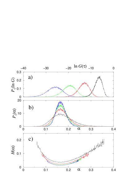
Figure 13: Probability distribution of the spin-spin correlation function for the 3-state diluted Potts model at criticality at the optimal dilution $p^{*}$. a) Probability distribution of the $\ln G_{\sigma}(\tau)$ for different distances along the strip, $\tau=50$, 100, 150 and 200 from right to left. b) Horizontal rescaling using the variable $\alpha=-\ln G_{\sigma}(\tau)/(2\pi\tau/L)$, with the same values of $\tau$ from top to bottom. c) Rough approximation of the universal spectral function which should no longer depend on the distance along the strip. It is given here at the saddle-point approximation, $H(\alpha)=-\frac{L}{2\pi\tau}\ln\left[\frac{L}{2\pi\tau}P_{\tau}(\alpha)\right]$.

Figure 14: Spectral function $H(\alpha)$ for $q=3$, 4, and 8 state per spin. The data corresponding to distances $\tau=50$, 100, 150 and 200 collapse onto single universal spectral functions. The multifractal spectrum becomes wider as $q$ is increased. At $q=3$, the solid lines are the results deduced from 1st and 2nd order expansions of $X_{\sigma^{n}}$ given in Refs. [6] and [13].

In the case of the diluted $3-$state Potts model, the probability distribution of the spin-spin correlation function at distances $\tau=50$, 100, 150, and 200 is presented in figure 13 (in fact $P_{\tau}(\ln G)$ is shown). As one can see, the distribution is very broad, and the broadening is more pronounced at large distances. We mention that the events corresponding to vanishing $G_{\sigma}(\tau)$ have been discarded (at $\tau=50$, it corresponds to $3\%$ of the events for $q=3$ ($22\%$ for $q=8$) and this proportion increases at $\tau=200$ to almost $5\%$ for $q=3$ (and $52\%$ for $q=8$)). A simple change to the natural variable $\alpha$ already produces a rescaling in the horizontal direction, and the spectral function deduced from the saddle-point approximation, $H(\alpha)=-\frac{L}{2\pi\tau}\ln\left[\frac{L}{2\pi\tau}P_{\tau}(\alpha)\right]$, is shown in the same figure. At this approximation, the maxima $P_{\tau}(\alpha_{0})$ should be given by $\frac{2\pi\tau}{L}$ (which take values close 157, 118, 78 and 40 for the values of $\tau$ chosen here). Since it is clearly not true (see figure 13 b) the minima of $H(\alpha)$ do not vanish and the rescaling is not perfect. We thus have to keep quadratic fluctuations about the saddle $n^{*}$ [58] leading to the following estimate of the Bromwich integral

$$P_{\tau}(\alpha)=\left[\frac{1}{2\pi}\left(\frac{\partial^{2}X_{\sigma^{n}}}{\partial n^{2}}\right)_{n^{*}}\right]^{-1/2}\left(\frac{2\pi\tau}{L}\right)^{1/2}\exp\left(-\frac{2\pi\tau}{L}H(\alpha)\right)$$ (27)

The rescaling is indeed clearly improved with

$$H(\alpha)=-\frac{L}{2\pi\tau}\ln\left[\left(\frac{L}{2\pi\tau}\right)^{1/2}P_{\tau}(\alpha)\right]$$ (28)

provided that the prefactor $\left[\frac{1}{2\pi}\left(\frac{\partial^{2}X_{\sigma^{n}}}{\partial n^{2}}\right)_{n^{*}}\right]^{-1/2}$ is of order unity. With the numbers taken from the maxima of figure 13 b), we deduce that at $q=3$ this prefactor takes a value close to $1.5$, making the correction term to equation (28), $\frac{L}{2\pi\tau}\ln\left[\frac{1}{2\pi}\left(\frac{\partial^{2}X_{\sigma^{n}}}{\partial n^{2}}\right)_{n^{*}}\right]^{-1/2}$, indeed negligible. This is also the case for $q=4$ and 8 and the spectral functions presented in figure 14 have a vanishing minimum and produce a very good rescaling of the correlation function probability distributions. The multifractal spectrum is broader at larger values of the number of states per spin, indicating a more important relative weight of the rare events, which implies that numerical results would become less reliable for large $q$’s.

5 Conclusion

We have studied the magnetic critical properties of the bidimensional diluted Potts model for $q=3$, 4, and 8. From transfer matrix computations, we obtained the critical exponents of the decay of the average spin-spin correlation function, $x_{\sigma}$, which are close to those obtained in the random-bond case. The maximum value of the central charge is found to be compatible with the estimates in the corresponding random-bond models. Finally, the multifractal spectrum of the diluted 3-state Potts model turns out to be compatible with that obtained both perturbatively and numerically for the random-bond case. This is a strong evidence of the existence of an unique fixed point for all kinds of disorder, even in the absence of duality symmetries. In which concerns the multifractal properties, the spectral function $H(\alpha)$ becomes broader when the number of states per spin increases, indicating extremely stretched probability distributions of the correlation functions.

References

References

- [1] A.B. Harris, J. Phys. C 7, 1671 (1974).
- [2] Y. Imry and M. Wortis, Phys. Rev. B 19, 3580 (1979).
- [3] M. Aizenman and J. Wehr, Phys. Rev. Lett. 62, 2503 (1989).
- [4] K. Hui and A.N. Berker, Phys. Rev. Lett. 62, 2507 (1989).
- [5] F.Y. Wu, Rev. Mod. Phys. 54, 235 (1982).
- [6] A.W.W. Ludwig, Nucl. Phys. B 285 [FS19], 97 (1987).
- [7] A.W.W. Ludwig and J.L. Cardy, Nucl. Phys. B 330 [FS19], 687 (1987).
- [8] A.W.W. Ludwig, Nucl. Phys. B 330, 639 (1990).
- [9] Vl. Dotsenko, M. Picco and P. Pujol, Nucl. Phys. B 455 [FS], 701 (1995).
- [10] Vik. Dotsenko, Vl. Dotsenko, M. Picco and P. Pujol, Europhys. Lett. 32, 425 (1995).
- [11] G. Jug and B.N. Shalaev, Phys. Rev. B 54, 3442 (1996).
- [12] Vik. Dotsenko, Vl. Dotsenko and M. Picco, Nucl. Phys. B250, 633 (1998).
- [13] M.A. Lewis, Europhys. Lett. 43, 189 (1998), Erratum, Europhys. Lett. 47, 129 (1999).
- [14] M. Picco, e-print cond-mat/9802092.
- [15] C. Chatelain and B. Berche, Phys. Rev. Lett. 80, 1670 (1998).
- [16] C. Chatelain and B. Berche, Phys. Rev. E 58, R6899 (1998).
- [17] G. Palágyi, C. Chatelain, B. Berche and F. Iglói, Eur. Phys. J. B 13, 357 (2000).
- [18] T. Olson and A.P. Young, Phys. Rev. B 60, 3428 (1999).
- [19] U. Glaus, J. Phys. A: Math. Gen. 20, L595 (1987).
- [20] J.L. Cardy and J.L. Jacobsen, Phys. Rev. Lett. 79, 4063 (1997).
- [21] M. Picco, Phys. Rev. Lett. 79, 2998 (1997).
- [22] J.L. Jacobsen and J.L. Cardy, Nucl. Phys. B 515, 701 (1998).
- [23] C. Chatelain and B. Berche, Phys. Rev. E 60, 3853 (1999).
- [24] C. Chatelain and B. Berche, Nucl. Phys. B 572, 626 (2000).
- [25] A. Roder, J. Adler, and W. Janke, Phys. Rev. Lett. 80, 4697 (1998).
- [26] A. Roder, J. Adler, and W. Janke, Physica A 265, 28 (1999).
- [27] Z.Q. Pan, H.P. Ying and D.W. Gu, arXiv:cond-mat/0103130
- [28] B. Derrida, Phys. Rep. 103, 29 (1984).
- [29] A. Aharony and A.B. Harris, Phys. Rev. Lett. 77, 3700 (1996).
- [30] S. Wiseman and E. Domany, Phys. Rev. Lett. 81, 22 (1998).
- [31] S. Wiseman and E. Domany, Phys. Rev. E 58, 2938 (1998).
- [32] Ch. V. Mohan, H. Kronmüller and M. Kelsch, Phys. Rev. B 57, 2701 (1998).
- [33] L. Schwenger, K. Budde, C. Voges and H. Pfnür, Phys. Rev. Lett. 73, 296 (1994).
- [34] E. Domany, M. Schick, J.S. Walker and R.B. Griffiths, Phys. Rev. B 18, 2209 (1978).
- [35] C. Rottman, Phys. Rev. B 24, 14821 (1981).
- [36] M. Sokolowski and H. Pfnür, Phys. Rev. B 49, 7716 (1994).
- [37] P. Piercy and H. Pfnür, Phys. Rev. Lett. 59, 1124 (1987).
- [38] W.C. Fan, A. Ignatiev and B. Hu, Phys. Rev. B 39, 6816 (1989).
- [39] H. Over, S. Schwegmann, G. Ertl, D. Cvetko, V. De Renzi, L. Floreano, R. Gotter, A. Morgante, M. Peloi, F. Tommasini and S. Zennaro, Surf. Sc. 376, 177 (1997).
- [40] K. Budde, L. Schwenger, C. Voges, and H. Pfnür, Phys. Rev. B 52, 9275 (1995).
- [41] C. Voges and H. Pfnür, Phys. Rev. B 57, 3345 (1998).
- [42] J.L. Cardy, M. Nauenberg and D.J. Scalapino, Phys. Rev. B 22, 2560 (1980).
- [43] H.W.J. Blöte and M.P. Nightingale, Physica (Amsterdam) 112A, 405 (1982).
- [44] P.W. Kasteleyn and C.M. Fortuin, J. Phys. Soc. Japan 26 Suppl., 11 (1969).
- [45] H. Furstenberg, Trans. Am. Math. Soc. 108, 377 (1963).
- [46] B. Nienhuis, J. Phys. A: Math. Gen. 15, 199 (1982).
- [47] H.W.J. Blöte, J.L. Cardy and M.P. Nightingale, Phys. Rev. Lett. 56, 742 (1986).
- [48] P. Reinicke, J. Phys. A: Math. Gen. 20, 5325 (1987).
- [49] S.L.A. de Queiroz, J. Phys. A: Math. Gen. 33, 721 (2000).
- [50] V. Dotsenko, J.L. Jacobsen, M.-A. Lewis and M. Picco, Nucl. Phys. B 546, 507 (1999).
- [51] J.L. Jacobsen and M. Picco, Phys. Rev. E 61, R13 (2000).
- [52] A.B. Zamolodchikov, JETP Lett. 43, 730 (1986).
- [53] U. Wolff, Phys. Rev. Lett. 62, 361 (1989).
- [54] L. Turban, Phys. Lett. 75A, 307 (1980).
- [55] L. Turban, J. Phys. C: Solid State Phys. 13, L13 (1980).
- [56] P. Guilmin and L. Turban, J. Phys. C: Solid State Phys. 13, 4077 (1980).
- [57] B. Fourcade and A.-M.S. Tremblay, Phys. Rev. A 36, 2352 (1987).
- [58] A. Aharony and R. Blumenfeld, Phys. Rev. B 47, 5756 (1993).