Patterns, Trends and Predictions
in stock market indices
and foreign currency exchange rates

Summary.

Specialized topics on financial data analysis from a numerical and physical point of view are discussed. They pertain to the analysis of crash prediction in stock market indices and to the persistence or not of coherent and random sequences in fluctuations of foreign exchange currency rates. A brief historical introduction to crashes is given, including recent observations on the DJIA and the S&P500. Daily data of the DAX index are specifically used for illustration. The method for visualizing the pattern thought to be the precursor signature of financial crashes is outlined. The log-periodicity of the pattern is investigated. Comparison of patterns before and after crash days is made through the power spectrum. The corresponding fractal dimension of the signal looks like that of a percolation backbone. Next the fluctuations of exchange rates (XR) of currencies forming $EUR$ with respect to $USD$ are analyzed. The XR power spectra are calculated before and after crashes. A detrended fluctuation analysis is performed. The characteristic exponents $\beta$ and $\alpha$ respectively, are compared, including the time dependence of each $\alpha$, found to be singular near crash dates.

1 An Introduction with Some Historical Notes as ”Symptoms”

The stock market crash on Monday Oct. 19, 1987 led to the October black monday syndrome. On that day, the Dow Jones Industrial Average (DJIA) lost 21.6 %. Other markets were shaken : the worst decline reached 45.8 % in Hong Kong. The downturn was spread out over two or three days in different European stock markets: the DAX lost 10 %. Nevertheless most markets had been using for a long time breakers, i.e. periods of trading halts and/or limitations of daily variations. This tends to suggest that the adoption of circuit breakers at the very least do delay the crash process, and not much more. In fact, Lauterbach and Ben-Zion lb1993 found that trading halts and price limits had no impact on the overall decline of October 1987, but merely smoothed return fluctuations in the neighborhood of the crash.

Another major characteristic of the crash of October 1987 is the phenomenon of irresistible contagion. It is well accepted that the shock arose first from Asian markets, except Japan, then propagated to the European markets before reaching the American markets after, when Asian markets were already closed Roll1989 . A mapping of the Nikkei, DAX and DJIA daily sign fluctuations has been made onto a 1/2 Ising spin chain as if there was a continuous index calculated three times during 24 hours. This showed that the spin cluster fluctuations are rather equivalent to random fluctuations, - except during pre-crash periods in which ($down-down-down$) spin clusters form with a higher probability than expected if the fluctuations are to be considered independent of each other domino . This has allowed to eliminate all criticisms about the major responsibility of the derivative markets in the United States on the Oct. 87 crash. Since then, the world-wide interdependence of the economy has been going on still more strongly. Thus if really a speculative bubble is occurring on some financial markets, as commonly observed in the recent years, the phenomenon of propagation to other stock exchanges could be more important now. It is known that methods of negotiation have widely changed on many financial places. Markets using electronic systems of negotiation take advantage of recent improvement in their transaction capacity. It is easier today to face a substantial increase in transaction volumes during a major crisis period. Moreover, the efficient use of the derivative markets could avoid useless pressures on the traditional market. These financial factual observations should be turned into quantitative measures, in order to, if necessary, avoid crashes.

Whence there is a need for techniques capable of rapidly following a bubble explosion or preventing it. Notice that the drop of stock market indices can not only spread out over two or three days but also over a much longer period. The example of the Tokyo stock exchange at the beginning of the 1990’s is a prominent illustration. By comparison to the most famous crash of 1929, the Oct. 87 crash was spread over 2 days: the Dow Jones sank 12.8 % on October 28 and 11.7 % on the following day. (That was similar for the DAX which dropped by 8.00 % and 7.00 % on Oct. 26 and 28, 1987 respectively.) This shows that a stock market index decline does not necessarily lead to a crash in one single day. Indeed, the decline can be slow and last several days or even several months in what would be called not a crash, but a long duration bear market.

In the present econophysics research context, it is of interest to examine whether the evolution of quotations on the main stock exchange places have similarities and whether crash symptoms can be found. Even if history generally tends to repeat, does it always do so in similar ways, and what are the differences? A rise in quotations can be interpreted a posteriori as the result of a speculative bubble but could be mere euphoria. How this does lead to a rupture of the trend? Can the duration differences be interpreted? Can we find universality classes?

Physics-like model of fracture or other phase transitions, including percolation can be turned into some economic advantage. Along the same lines of thought, the question was already touched upon in bigtokyo within the sand pile model. This allows not only a verbal analogy of index rupture in terms of sand avalanches, but also some insight into the mechanisms. Through physical modeling and an understanding of parameters controlling the output, as in the sand pile model, symptoms can be measured, whence to suggest remedies is not impossible.

Another question raised below is the post-crash period. One might expect from a physics point of view that if a crash looks like a phase transition, and is characterized by scaling laws, as we will see it sometimes occurs SJB96 ; phasetr , it might be expected that a relation exists between amplitudes and laws on both sides of the crash day roehner4 . As mentioned above, the crash might be occurring on various days, with different breaks. It might be possible that between drops some positive surge might be found. Thus some sorting of behaviors into classes should be made as well. In fine, some discussion on the foreign exchange market will be given in order to recall the detrended fluctuation analysis method, so often used nowadays. It is applied below to the $USD$ exchange rate vs. the (ten) currencies forming the $EUR$ on Jan. 01, 2000, over a time interval including the most recent years. The observation of the time variation of the power law scaling exponent of the DFA function is shown to be correlated to crash time occurrence.

1.1 Tulipomania

In 1559, the first tulip bulb (TB) was brought to Holland from China by Conrad Guenster webtulip . In 1611, the tulip bulbs (TBs) were stocked and sold on markets. In 1625, one tulip bulb was worth 5 dutch gulden (NLG). The flower was considered so rare that wealthy aristocrats and merchants tripped over themselves to buy the onions. Speculation ensued and the TBs became wildly overvalued. The TBs were not necessarily planted, but were just stored in the house salon. In 1635, 1 TB was worth 4 tons of wheat + 4 oxen + 8 tons rye + 8 pigs + one bed + 12 sheep + clothes + 2 wine casks + 4 tons beer + 2 tons butter + 1000 pounds cheese + 1 silver drinking cup. In 1637, 1 TB was worth 550 NLG. One average house was worth 17 800 NLG, whence about 30 TBs. However within 1637, over a 6 week time span the price of 1 TB went down 90 %.

In view of the shock, remedies had to be found and people called upon the Amsterdam Parliament for legislation. It was decided that all contracts would be void if they were dealt before Nov. 1636, and after that date the contracts kept a 10 % value. Under some protest, people appealed to the Netherland Supreme Court which ruled that this business of selling/buying TBs was mere gambling, and no debt could be defined ”by law” nor ruled upon. Nowadays one TB is worth 0.5 EUR. Too bad for long term investment strategies. The TB became the classical example for illustrating the Extraordinary Popular Delusions and the Madness of Crowds as described by Charles MacKay webmackay .

Just for the sake of physics history, let it be recalled that 1639 was the year in which Galileo Galilei (Pisa, Feb. 15, 1564; Arcetri, Jan. 8, 1642) betrayed science in saving his life.

1.2 Monopolymania

Another set of financial crises is that of the Compagnie du Mississipi weblaw and that of the South Sea Company websouthsea1 ; websouthsea2 . In 1715, John Law, a scot gambler, had persuaded Philippe, Regent of France, to consider a banking scheme that promised to improve the financial condition of the kingdom. In theory a private affair, the system was linked from the beginning with liquidating the national debt. When the monopoly of the Louisiana trade was surrendered in 1717, Law created a trading company known as the Compagnie d’Occident (or Compagnie du Mississipi) linked to the Royal Bank of France (first chartered in 1716 as Banque Générale) and in which government bills were accepted for the purchase of shares.

Law gained a monopoly on all French overseas trade. The result was a huge wave of speculation as the value of a share went from its initial value, i.e. 500 livres to 18 000 $livres$. When the paper money was presented at the bank in exchange for gold, which was unavailable, panic ensued, and shares felt by a factor of 2 in a matter of days.

In England, the Whigs represented the mercantile interests which had profited from the War of the Spanish Succession War (1703-1711), and made large profits by financing it, in doing so had created a National Debt which had to be financed by further taxation. During the wars the government handled more money than ever before in history, and they skimmed off a lot through various methods, including the invention of the Bank of England in 1694. The South Sea Company was formed in 1711 by the Tory government of Harley to trade with Spanish America, and to offset the financial support which the Bank of England had provided for previous Whig governments. They had in mind to establish a system like the Compagnie du Mississipi Monopoly, weblaw using the same sort of trading privileges and monopolies, those granted to Britain after the Treaty of Utrecht. King George I of Great Britain became governor of the company in 1718, creating confidence in the enterprise, which was soon paying 100 percent interest. In 1720 a bill was passed enabling persons to whom the government owed portions of the national debt to exchange their claims for shares in company $stocks$, and to become stock holders. In the 1719-20 the England Public Debt went to South Sea Company stock holders, as approved by Parliament. On March 1 the stocks were valued GBP 175, moved quickly to 200. Shortly the directors of the South Sea Company had assumed three-fifths of the national debt. The company expected to recoup itself from expanding trade, but chiefly from the foreseen rise in the value of its shares. On June 1 the shares were valued 500 and more than 1,000 in August 1720. Those unable to buy South Sea Company stocks were inveigled by overly optimistic company promoters or downright swindlers into unwise investments. Speculators took advantage of investors to obtain subscriptions for sensibly unrealistic projects. By September 1720 however, the market had collapsed, and by December 1720 South Sea Company shares were down to 124, dragging others, including government stocks with them. Many investors were ruined, and the House of Commons ordered an inquiry, which showed that ministers had accepted bribes and speculated. From a physics point of view let it be recalled that I. Newton (Woolsthorpe, Dec. 25, 1642; London, March 20, 1727) invested in such South Sea Company stocks and lost quite a bit of money Newton .

1.3 WallStreetmania

In the years from 1925 to 1929 one could easily go to a broker and purchase stocks on margin, i.e. instead of buying stocks with real cash money, one could purchase them with some cash down and the rest on credit. The Coolidge administration had a laissez-faire policy, i.e. a government policy of non-intervention. It was almost la façon de vivre to play in the stock market wallstreetcrash29 . That allowed a speculation bubble to grow unchecked. The Federal Reserve powers on economic matters were not utilized as could be done nowadays. Many successions of $mini$ crashes and rallies began as early as March 1929. The summer of 1929 hearkened somewhat of the good old days of optimism. The market appeared to be stable. On Sept. 3, a bear market became firmly established, and on Thursday Oct. 24, 1929 the famous 1929 crash occurred (Fig. 1).

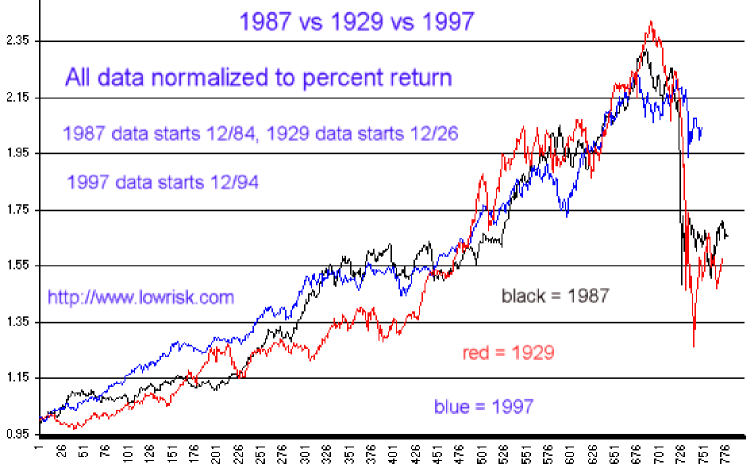
Figure 1: Famous Wall Street Crashes : 1929, 1987, 1997; taken from color web site http://www.lowrisk.com/crash/87vs97.htm; from top to bottom on day 201 : blue (97), red (29), black (87); on day 700 : red (29), black(87), blue(97)

The 1987, 1997, and more recent 1999, 2000, 2001 crashes are reminiscent and even copies of the above ones (Fig. 1). The symptoms look similar : artificially built euphoria, malingnantly established speculation, easy access to market activities, including manipulated (or rather $electronipulated$) informations … Consider the buying frenzy on IPOs stocks at the end of the 1990’s in companies for which owners do not have a coherent business plan, or are not going to make money, … and yet see how we bought e-stocks. Nothing has changed since 1600, 1700 nor 1929.

2 Econophysics of Stock Market Indices

Econophysics ausloos ; contwille aims to fill the huge gap separating ”empirical finance” and ”econometric theories”. Various subjects have been approached like the option pricing, stock market data analysis, market modelling and forecasting, etc…The application of statistical physics ideas to the forecasting of stock market behavior has been proposed earlier following the pioneer work of physicists interested by economy laws mandel ; stanley ; bouch ; peters1 ; peters2 ; MantegnaStanleybook ; voit .

Even though a stock market crash is considered as a highly unpredictable event, it should be reemphasized that it takes place systematically during a period of generalized anxiety spreading over the markets following a euphoria time. The crash can be seen as a natural correction bringing the market to a ”normal state”. Three important facts should be underlined:

(i) The series of daily fluctuations, so called $volatility$, of the stock market presents a huge clustering around the crash date, i.e. huge fluctuations are grouped around the crash date. This is well illustrated in Fig. 2 for the case of the DAX around 1987. The time span of this clustering is quite long: a few years. This clustering indicates that larger and larger fluctuations take place before crashes.

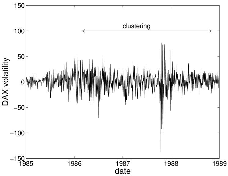
Figure 2: DAX volatility between Jan. 01, 85 and Dec. 31, 88

(ii) Collective effects are to be considered, be they stemming from macroeconomy informations, as a set of ”external fields”, and leading to a bear market, or more intrinsically $self-organized$, as if microeconomic informations (or $interactions?$) were triggering the non-equilibrium state evolution.

(iii) A third remark concerns the panic–correlations appearing before crashes. This kind of collective behavior is commonly observed during a trading day. The market in Tokyo closes before London opens and thereafter New York opens. During periods of panic, financial analysts are looking for the results and evolution of the geographically preceding market. Strong correlations are found in fluctuations of different market indices before crashes.

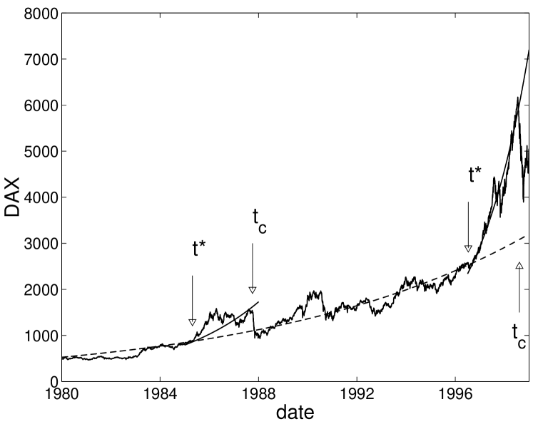
Figure 3: DAX evolution between Jan.01, 1980 and Dec.31, 1998 with the mean field behavior, the time(s) $t^{*}$, corresponding to the $Ginzburg-Levanyuk$ temperature bounding the critical fluctuation region, and the critical crash day(s) $t_{c}$

Of course, fluctuations and correlations are both ingredients which are supposedly known to play an important role in phase transitions. Thus an analogy can be derived (Fig.3) between phase transitions and crashes, defining the mean field (exponential-like) behavior, the time $t^{*}$, corresponding to the $Ginzburg-Levanyuk$ temperature bounding the critical fluctuation region, the critical crash day $t_{c}$, etc. phasetr . The character of a thermodynamic phase transition is characterized by critical exponents, following the scaling law hypothesis, exponents which are thought to depend on the symmetry of the order parameter and the underlying lattice dimensionalityStanleyPTbook . Similar considerations are looked for in financial crash studies.

In 1996, two independent works sornette ; FF96 have proposed that critical phenomena would be possible scenarios for describing crashes. Those authors are still debating about the subject sornette2 ; feig2 . More precisely, it has been proposed that an economic index $y(t)$ increases as a power law decorated with a log-periodic oscillation, i.e.

$$y=A+B{\left({t_{c}-t\over t_{c}}\right)}^{-m}\left[1+Csin\left(\omega\ln{\left({t_{c}-t\over t_{c}}\right)}+\phi\right)\right]\hskip 8.5359ptfor\hskip 8.5359ptt<t_{c}$$ (1)

where $t_{c}$ is the crash-time or rupture point, $A$, $B$, $m$, $C$, $\omega$ and $\phi$ are free parameters. This evolution $y(t)$ is in fact the real part $\Re$ of a power law behavior at $t=t_{c}$ with a complex exponent $m+i\omega$, i.e.

$$y\sim\Re\left\{{\left(t_{c}-t\over t_{c}\right)}^{-m+i\omega}\right\}$$ (2)

The law for $y(t)$ diverges at $t=t_{c}$ if $m>0$. This evolution is decorated with oscillations converging at the rupture point $t_{c}$. This law is similar to that of critical points, and generalizes the situation for cases in which a hierarchical lattice structure exists, in other words a Discrete Scale Invariance (DSI) is subjacent dsi .

The relationship (1) has been proposed elsewhere in order to fit experimental measurements of sound wave rate emissions prior to the rupture of heterogeneous composite stressed up to failure fracture . The same type of complex power law behavior has been also observed as a precursor of the Kobe earthquake in Japan kobe . Such log-periodic corrections have been recently reported in biased diffusion on random lattices bias .

As early as April 1997, Vandewalle and Ausloos performed a series of investigations in order to emphasize crash precursors dup1 ; cash1 ; vif . The closing values of the Dow Jones Industrial Average (DJIA) and the Standard & Poor 500 (S&P500) were used for tests. A law slightly different from Eq.(1) was proposed dup1 ; how . A strong indication of a so-called crash event or market rupture point was numerically discovered dup1 ; cash1 ; vif ; how . Further data analysis (in Aug. 97) dup2 including a risk measure cash2 indicated a crash to occur in between the end of October 1997 and mid-November 1997. The crash occurred effectively on Monday October 27th, 1997 how !

Eventhough the crash of October 1997 was predicted how ; dup2 , the scientific (physics or economy) critics ; nonos and media vif community is actually divided between those who believe in such a crash prediction and those who believe that crashes are unpredictable events and such findings were mere luck or at best accidental sornette2 ; feig2 ; brisbois . We discuss a little bit more the predictability problem and findings in this paper going beyond a previous report bigtokyo .

2.1 Methodology and data analysis

In e.g. Refs.bigtokyo ; viz ; ladek ; jura , the fact was underlined that there are strong physical arguments stipulating that $m$ in Eq. (1) could be or even should be taken as ”universal”. The universal $m=0$ value, i.e. a logarithmic divergence has been proposed. The logarithmic divergence of the index $y$ for $t$ close to $t_{c}$ reads

$$y=A+B\ln{\left({t_{c}-t\over t_{c}}\right)}\left[1+Csin\left(\omega\ln{\left({t_{c}-t\over t_{c}}\right)}+\phi\right)\right]\hskip 8.5359ptfor\hskip 8.5359ptt<t_{c}.$$ (3)

One should remark that the full period $[t_{i},t_{f}]$ for a meaningful fit should contain the whole euphoric precursor. It has been found in bigtokyo ; how ; ladek ; jura that the log-divergence is closer to the real signal than any power law divergence with $m$ $\neq$ 0.

The log-divergence in Eq.(3) contains 6 parameters. At first, it seems that non-linear fits using only the simple log-divergent function

$$y=A+B\ln{(t_{c}-t)}$$ (4)

with $B<0$, thus with only 3 parameters can be performed. A good estimation of $t_{c}$ can be obtained indeed following both Levenberg-Marquardt and Monte-Carlo algorithms recipes . One has observed that the estimated $t_{c}$ points are close to ”black” days for the first two periods bigtokyo ; ladek ; jura .

Assuming that Eq.(4) is valid, one should also note that

$${dy\over dt}={-B\over(t_{c}-t)}$$ (5)

should be found in the daily fluctuation pattern (Fig. 2). This is consistent with the volatility clustering discussed here above. However, Eq.(5) fits lead to bad results with huge error bars.

The oscillating term of Eq.(3) has been quite criticized since no traditional or economical argument supports the DSI theory at this time. However, the hierarchical structure of the market has been suggested as a possible candidate for generating DSI patterns in bigtokyo ; FF96 ; hierarchy ; FF98 ,so is the price fixing ”techniques” roehner3 and arbitrage methods. In order to prove that a log-periodic pattern appears before crashes, the envelope of the index $y$ is constructed viz . Two distinct curves are built: the upper envelope $y_{max}$ and the lower one $y_{min}$. The former represents the maximum of $y$ in an interval $[t_{i},t]$ and the latter is the minimum of $y$ in an interval $[t,t_{f}]$. One observes a remarkable pattern made of a succession of thin and huge peaks viz .

When $y_{max}-y_{min}=0$, it means that the index $y$ reaches some value never reached before at a time $t$ and would never have reached if the time axis had been reversed thereafter. This corresponds to time intervals during which the value of the index $y$ reaches new records. In fact, the pattern reflects obviously an oscillatory precursor of the crash, thus through

$$y_{max}-y_{min}=(C_{1}+C_{2}t)(1-\cos{(\omega\ln{(t_{c}-t)}+\phi)})$$ (6)

where $C_{1}$ and $C_{2}$ are parameters controlling the amplitude of the oscillations. The above relationship allows us to measure the log-frequency $\omega$ viz . Moreover it is found that the value of $\omega$ seems to be finite and almost constant, $\omega\simeq[6,10]$ for the major analyzed crashes. An analysis along similar lines of thought, though emphasizing the no-divergence, thus $m<0$ in Eqs. (1)-(2), was discussed for the Nikkei sornettenikkei ; stauijtaf and NASDAQ April 2000 crash sornetteNASDAQ .

For illustrating the complexity of the frequency dependence of such financial signals, one can also perform a Fourier transform of a reconstructed signal. The evolution of the six strongest DAX crashes between Oct. 01, 1959 and Dec. 31, 1988 and the strongest DAX crashes in 1997, prior to the crash day, are shown in Fig. 4; $y_{0}$ denotes the index value at the closing of the crash day. Power spectra of the DAX index measured from the index value at the end of the crash day have been calculated for a time interval equal to 600 days, those prior to crashes. The 6 large DAX crash spectra for the period of interest are shown in Fig. 5. The corresponding exponents $\beta$ for the best fit in the high frequency region are given in Table 1.

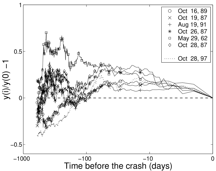
Figure 4: The evolution of the six strongest DAX crashes between Oct. 01, 59 and Dec. 31, 88, and the strongest DAX crash in 1997, prior to the crash day ; $y_{0}$ denotes the index value at the closing of the crash day

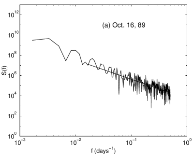
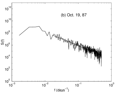
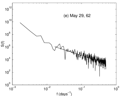
Figure 5: The power spectrum of the 600 day DAX index evolution signal corresponding to the six major crashes between Oct. 01, 59 and Dec. 31, 96

The roughness behavior schroeder ; west ; chemnitz of the DAX index evolution signal before crashes can be defined trough the fractal dimension $D$ of the signal, i.e. schroeder

$$D=E+\frac{3-\beta}{2},$$ (7)

where $E$ is the Euclidian dimension. The values of $\beta$ and $D$ are reported in Table 1 with the crash dates and relative amplitude of the 6 major DAX crashes which occurred between Oct. 01, 1959 and Dec. 30, 1996. The same type of data is reported in Table 2 for the 3 major DAX crashes in October 1997. The power spectrum of the large Oct. 28, 97 crash is shown in Fig. 6.

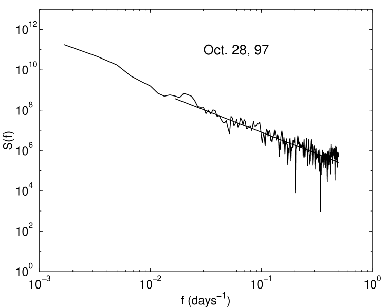
Figure 6: The power spectrum of the 600 day DAX index evolution signal prior to the Oct. 28, 97 crash

Table 1: Crash dates and relative amplitude of the 6 major DAX crashes having occurred between Oct. 01, 1959 and Dec. 30, 1998; power law exponent $\beta_{-}$ of the signal power spectrum (600 data points) and corresponding fractal dimension $D_{-}$ of the signal prior to, and $\beta_{+}$ and $D_{+}$, after these 6 major DAX crashes.

crash dates	relative amplitude	$\beta_{-}$	$D_{-}$	$\beta_{+}$	$D_{+}$
16.10.89	-0.137	1.90$\pm$0.09	1.55	1.67$\pm$0.09	1.67
19.10.87	-0.099	2.24$\pm$0.09	1.38	1.82$\pm$0.09	1.59
19.08.91	-0.099	1.82$\pm$0.10	1.59	1.62$\pm$0.06	1.69
26.10.87	-0.080	2.00$\pm$0.09	1.50	1.70$\pm$0.08	1.65
29.05.62	-0.075	1.77$\pm$0.08	1.62	1.28$\pm$0.08	1.86
28.10.87	-0.070	1.94$\pm$0.10	1.53	1.81$\pm$0.07	1.60

Table 2: The 3 major DAX crashes in October 1997 : crash dates, relative amplitude, power law exponent $\beta_{-}$ of the signal power spectrum (600 data points prior to these 3 major DAX crash dates) and the corresponding fractal dimension $D_{-}$.

crash dates	relative amplitude	$\beta_{-}$	$D_{-}$
28.10.97	-0.084	2.14$\pm$0.07	1.43
27.10.97	-0.043	1.97$\pm$0.07	1.52
23.10.97	-0.048	1.91$\pm$0.05	1.55

2.2 Aftershock patterns

The index evolution after a crash has also been analyzed through a reconstructed signal that is the difference between the DAX value signal at each day $y(i)$ and the DAX value at the crash day $y_{0}$. For the 6 largest crashes in the time interval of interest the recovery can be slow (Fig.7). It took about one month for the Oct. 28, 97 crash. To observe some periodic fluctuation after the crash, the power spectrum of the DAX has been computed for the 600 days following a crash day (Fig. 8 (a-f)). Note the high-frequency log-periodic oscillation regime of the power spectrum for the Oct. 19, 1987 case on Fig. 7(d). The values of each $\beta$ and corresponding fractal dimension $D$ are reported in Table 1.

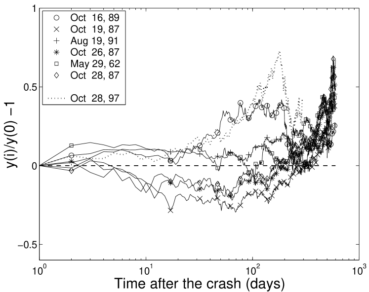
Figure 7: The DAX recovery signal evolution after the six strongest DAX crashes having occured between Jan. 01, 85 and Dec. 31, 88, and after the strongest DAX crash in 1997 ; $y_{0}$ denotes the index value at the closing of the crash day

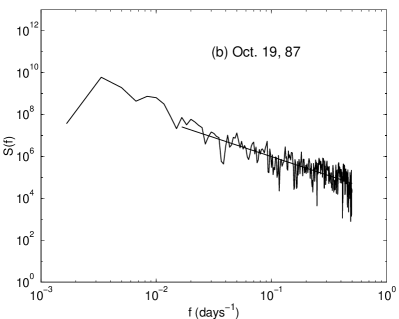
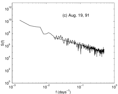
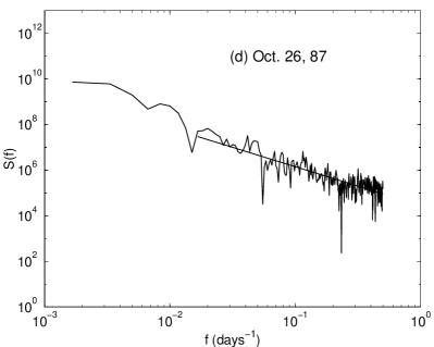
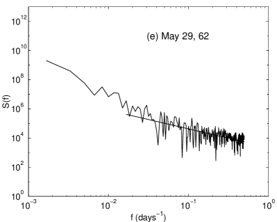
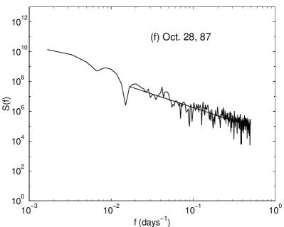
Figure 8: The power spectrum of the 600 day DAX index evolution signal after the six major crashes having occured between Oct. 01, 59 and Dec. 31, 96

As a final point of this section, it should be noticed that the fractal dimension is close to 1.70, thus very similar to that of a percolation backbone. This might be the hint that hierarchical structures are present, and a cause of crashes. As a consequence, the market could be viewed as a discrete fractal system, transiting at crashes like a physical system at a percolation transition.. In related work, Amaral and coworkers amaral have studied the statistics of several companies as well as their respective growth. They have found that the growth of companies can be modelled using a hierarchical lattice like a Cayley tree. For simple models of hierarchically organized markets some self-regulation is found in fact sopthierarchy . On such systems the fractal dimension can be considered to have an imaginary part which is related to the log-periodic oscillations, - in fact is the signature of the branching ratio fractaltree .

In conclusion of this section, we may conjecture that stock markets are also hierarchical objects where each level may have a different weight, connectivity, and characteristics time scale (the horizons of the inve stors) bigtokyo . The hierarchical tree might be fractal at crashes and its geometry might control the type of criticality. This gives some argument in favor of the sand pile model on a fractal basis fractalsand as a microscopic model actually able to simulate a crash bigtokyo .

3 Foreign Currency Exchange Rates

Beside the crash cases discussed here above numerous examples of scale invariance seem to be widespread in natural and social systems west ; bakbook . A fundamental problem is the existence and width of the scaling range for long-range power-law correlations (LRPLC) in economic systems, as well as the presence of economic cycles. Indeed, traditional methods (like spectral methods) have corroborated the evidence that the Brownian motion idea or ordinary random walk is quite away from reality and LRPLC quite frequent stanley ; peters1 ; MantegnaStanleybook ; voit . Different approaches chemnitz have been envisaged to measure the LRPLC or analyze them in financial data: tails of partial distribution functions of the volatility, wavelet analysis, Detrended Fluctuation Analysis (DFA) DNADFA , etc.

3.1 DFA analysis

The DFA method DNADFA consists in dividing the whole data sequence $y(n)$ of length $N$ into $N/\tau$ non overlapping boxes, each containing $\tau$ points. Then, the local trend

$$z(n)=an+b$$ (8)

in each box is defined to be the ordinate of a linear least-square fit of the data points in that box. One should remark that a trend $z(n)$ different from a first-degree polynomial can also be used like the cubic trend ndub . Other detrending functions may improve the accuracy of the DFA technique, sort out the reason for crossovers between scaling regimes, and pin point noise and intrinsic trends hu .

The so-defined detrended fluctuation function $F(\tau)$ is then calculated following

$${{F(\tau)}^{2}}={1\over\tau}{\sum_{n=kt+1}^{(k+1)\tau}{|y(n)-z(n)|}^{2}},{\hskip 28.45274pt}k=0,1,2,\cdots,\left({N\over\tau}-1\right)$$ (9)

Averaging $F(\tau)$ over the $N/\tau$ intervals gives a function depending on the box size $\tau$. The above calculation is repeated for different box sizes $\tau$. If the $y(n)$ data are randomly uncorrelated variables or short range correlated variables, the behavior is expected to be a power law

$$\langle F(\tau)^{2}\rangle^{1/2}\sim\tau^{\alpha}$$ (10)

with an exponent 1/2 DNADFA if the excursion is governed by a mere random walk. An exponent $\alpha\not=1/2$ in a certain range of $\tau$ values implies the existence of LRPLC in that time interval. Mathematically, the correlation of a future increment $y(n)-y(0)$ with a past increment $y(0)-y(-n)$ is given by

$$\Gamma(n)={\langle(y(0)-y(-n))(y(n)-y(0))\rangle\over\langle(y(n)-y(0))^{2}\rangle}=2^{2\alpha-1}-1,$$ (11)

where the correlations are normalized by the variance of $y(n)$. For $\alpha>1/2$, there is persistence, i.e. $\Gamma>0$. In this case, if in the immediate past the signal has a positive increment, then on the average an increase of the signal in the immediate future is expected. In other words, persistent stochastic processes exhibit rather clear trends with relatively little noise. An exponent $\alpha<1/2$ means antipersistence, i.e. $\Gamma<0$. In this case, an increasing value in the immediate past implies a decreasing signal in the immediate future, while a decreasing signal in the immediate past makes an increasing signal in the future probable. In so doing, data records with $\alpha<1/2$ appear very noisy (rough). The $\alpha=0$ situation corresponds to the so-called white noise. Finally, one should note that $\alpha$ is nothing else than $Ha$, the so-called Hausdorff exponent for fractional Brownian motions west ; chemnitz . It can be useful to recall chemnitz that the power spectrum of such random signals is characterized by a power law with an exponent $\beta=2\alpha-1$.

3.2 Data and analysis

We have considered the daily evolution of several currency exchange rates with respect to the $USD$ from January 1990 till December 1999 including only all open banking days. This represents about $N=3000$ data points. The data are those obtained from quoteEUR , at the closing time of the foreign exchange market in London for the ten currencies $C_{i}$, (i=1,10) forming the $EUR$ on Jan. 01, 1999.

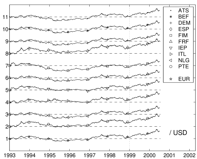
Figure 9: Normalized $EUR$ and $C_{i}$ (i=1,10) currency forming the $EUR$ exchange rates with respect to the $USD$ between Jan. 01, 1993 and June 30, 2000. The data are artificially multiplied by two and then displaced along the vertical axis in order to make the fluctuations noticeable. The vertical dash line marks the date for the EUR official introduction

The evolution of such $C_{i}$/$USD$ exchange rate from Jan. 01, 1993 to June 30, 2000 is drawn in Fig. 9. In Fig. 10, a log-log plot of the 10 functions $\langle F(t)^{2}\rangle^{1/2}$ is shown for the whole data of Fig. 9. Moreover we plot the result for a false $EUR$, i.e. a linear combination of the ten currencies forming the $EUR$ Ref1EUR ; kimalg ; tokyokima ; ijmpc Except for $IEP$, the functions are very close to a power law with an exponent $\alpha=0.51\pm 0.02$ holding over two decades in time, i.e. from about one week to two years. This finding clearly shows the non-existence of LRPLC in the foreign exchange market with respect to the $USD$. Other cases showing marked deviations from Brownian motion have been discussed elsewhere kimalg ; ijmpc ; nvma ; h1c1 . It can then be observed that a wide variety of behaviors is found in the foreign currency exchange market. Exponent values and the range over which a power law holds drastically vary from a currency exchange rate to another. It appears that the currency exchange rates can be classified into three different categories from the LRPLC point of view.

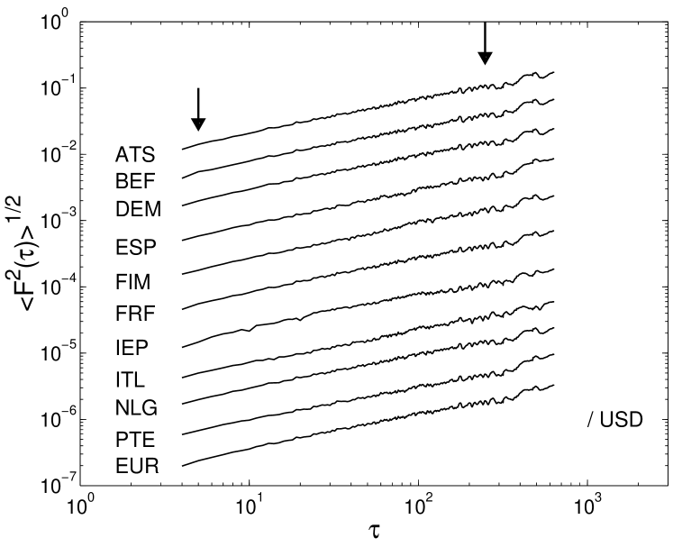
Figure 10: Log-log plot of the DFA function showing how to obtain the $\alpha$ exponent for the 11 exchange rates of interest for $EUR/USD$. The fit slope being only of interest, the DFA function data has been arbitrarily displaced along the vertical axis

First, the rates which exhibit an exponent $\alpha$ larger than 1/2 (persistent behavior). This case corresponds to currency exchange rates between leading currencies (e.g., $USD$, $JPY$, $EUR$) and so called $weaker$ ones h1c1 ; kiagina .

A second category concerns the rates exhibiting strict randomness ($\alpha=1/2$) within error bars. This is the case for example of the $USD/{C_{i}}$ rates as shown above.

A third category represents the currency exchange rates with antipersistent behavior ($\alpha<1/2$) as e.g. $DEM/BEF$ nvma . These currencies most often concern currency exchange rates between (european) countries which are submitted to strict monetary rules and to strict regulatory corrections by central banks due to international multilateral conventions. It should be pointed out that in general the range, over which the antipersistency signature, i.e. the power law is valid, occurs over a limited time span in this third category. In fact, there is a crossover around $\tau^{*}\approx 10$ weeks. For longer time scales ($\tau>>\tau^{*}$), the signal becomes again persistent or random.

3.3 Probing the local correlations

It is also of interest to know whether the LRPLC are stable along the data. In order to probe the local strength of the correlations, one constructs a so-called observation box of width $T$ placed at the beginning of the data, and calculates $\alpha$ for the data contained in that box. Then, the box is moved along the data by some step toward the right along the financial sequence and $\alpha$ is again calculated. Iterating this procedure one obtains a ”local measurement” of the degree of ”long-range correlations” over $T$. It is crucial to choose the most adequate box size $T$, i.e. to choose $T$ of the same order of magnitude as the maximum range $\tau$ over which the above power law is valid.

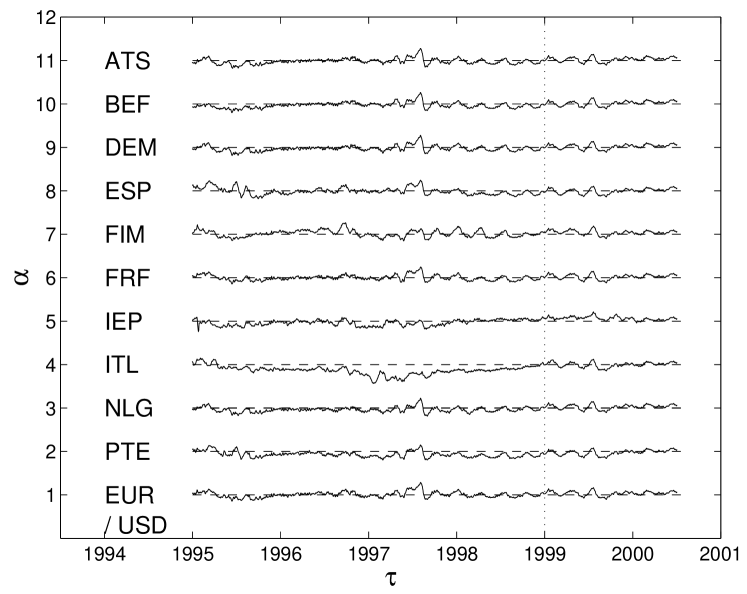
Figure 11: Time dependence of the DFA $local$ $\alpha$-exponent for $EUR$ and each currency forming the $EUR$ exchange rate with respect to $USD$. The $\alpha$-values are artificially multiplied by two and then displaced along the vertical axis in order to make the fluctuations noticeable. For each time dependent $\alpha$ a horizontal dashed line is drawn to indicate a reference to Brownian fluctuations

The evolution of the $EUR/USD$ and $C_{i}/USD$ $\alpha$’s for the 1995-2000 period is illustrated in Fig. 11. In order to probe the local values of $\alpha$, we have used a window of size $T=2$ years. The exponent $\alpha$ varies around 1/2, i.e. the horizontal dashed line in Fig.10. The local value of $\alpha$ seems to decrease at first and regrows in 95, is stable in 96, has a big fluctuation in mid/fall 97 and becomes pretty stable thereafter. The ITL case evolution is slightly different. The minute differences have probably to be associated to national political or economic events having an impact on the international monetary policy. It seems interesting to notice that the large fluctuations in $\alpha$ occur just before the crash dates of stock market indices. See also the marked singularity in mid 1999, a signature of the XR’s adjustments prior to the EUR introduction. In order to further prove this point, a linear DFA analysis of the Dow Jones Industrial stock index around the 1987 October crash was performed nvmaunpublished . A similar pattern is found.

Other XR time series have been examined in order to check the non-stationarity of $\alpha$ kimalg ; ijmpc . This does support the idea that the foreign currency exchange markets are mainly governed by random conditions friedrich or is said to be efficient in more usual economic language. However, this unconditional randomness cannot be extrapolated to speculating times nor emerging currencies kilev . Different universality classes thereby emerge. It may be useful to recall that Hartmannhartmann has examined the competition between $USD$ and $EUR$ in a more general (political and economy) framework.

4 Conclusions

The DAX has been analyzed from the point of view of crashes, in particular the correlations in the signal volatility, before and after the critical days. The search for the crash day is separated into two numerical problems, that of the index divergence itself and that of the index oscillation frequency acceleration on the other hand. By considering the envelope of the DAX, we have demonstrated that before crashes, a log-periodic pattern exists. Even though error bars are intrinsically large, it is surprising to see that a rupture point is easily predicted. A hierarchical structure close to a fractal percolation backbone (or tree) seems intrinsic at crashes. The stability of this result should be tested in real time for the best future of our economic system. A few foreign exchange currency rates with respect to the $USD$ have been examined in order to illustrate the DFA technique, the intrinsic structure of the DFA exponent, and its implications with respect to crashes.

Acknowledgements

Luc T. Wille is gladly thanked for inviting us to present the above results and considerations, and enticing us into writing this report. Thanks to the State of Florida for some financial support allowing the authors to participate in the conference. MA thanks N. Vandewalle for numerous discussions.

References

- (1) B. Lauterbach, U. Ben-Zion: J Finance 48, 1909 (1993)
- (2) R. Roll: ’The International Crash of October 1987’, R. W. Kamphuis et al., eds.: Black Monday and the Future of Financial Markets, (Dow Jones/Irwin, Homewood, IL, 1989)
- (3) N. Vandewalle, Ph. Boveroux, F. Brisbois: Eur. J. Phys. B 15, 547 (2000)
- (4) M. Ausloos, K. Ivanova: ‘Crashes : symptoms, diagnoses and remedies’. In Empirical sciences in financial fluctuations, Tokyo, Japan, Nov. 15-17, 2000 Proceedings (Springer Verlag, Berlin, 2001) in press.
- (5) D. Sornette, A. Johansen, J.P. Bouchaud: J. Physique. I (France) 6, 167 (1996)
- (6) N. Vandewalle, Ph. Boveroux, A. Minguet, M. Ausloos: Physica A 255, 201 (1998)
- (7) B.M. Roehner: Eur. Phys. J. B 17, 341 (2000)
- (8) http://www.historyhouse.com/stories/tulip.htm
- (9) http://www.litrix.com/madraven/madne004.htm
- (10) http://www.enlou.com/people/bio-lawj.htm
- (11) http://landow.stg.brown.edu/victorian/history/ssbubble.html
- (12) http://www.britannica.com/eb/article?eu=70665&tocid=0
- (13) R. Westfall: The Life of Isaac Newton, (Cambridge Univ. Press, Cambridge 1994)
- (14) http://mypage.direct.ca/r/rsavill/Thecrash.html
- (15) M. Ausloos: Europhysics News, 29, 70 (1998)
- (16) R. Cont: In Statistical Physics on the Eve of the 21st Century , ed. by M.T. Batchelor and L. T. Wille, (World Scientific, Singapore, 1999) 47-64
- (17) B.B.Mandelbrot: J. Business 36, 349 (1963)
- (18) R.N.Mantegna, H.E.Stanley: Nature 376, 46 (1995)
- (19) J.-P.Bouchaud, D.Sornette: J. Phys. I (France) 4, 863 (1994)
- (20) E.E. Peters: Fractal Market Analysis : Applying Chaos Theory to Investment and Economics, (Wiley Finance Editions, New York, 1994)
- (21) E.E. Peters: Chaos and Order in the Capital Markets : A New View of Cycles, Prices, and Market Volatility, (Wiley Finance Editions, New York, 1996)
- (22) R.N. Mantegna, H.E. Stanley: An Introduction to Econophysics, (Cambridge Univ. Press, Cambridge, 2000)
- (23) J. Voit: The Statistical Mechanics of Financial Markets, (Springer, Berlin, 2001)
- (24) H.E. Stanley: Phase transitions and critical phenomena (Clarendon Press, London 1971)
- (25) D. Sornette, A. Johansen, J.-P. Bouchaud: J. Phys. I (France) 6, 167 (1996)
- (26) J.A. Feigenbaum, P.G.O. Freund: Int. J. Mod. Phys. B 10, 3737 (1996)
- (27) D. Sornette, A. Johansen: Quantitative Finance 1 452 (2001)
- (28) J.A. Feigenbaum: Quantitative Finance 1 346 (2001)
- (29) D. Sornette: Physics Reports 297, 239 (1998)
- (30) J.C.Anifrani, C.Le Floc’h, D.Sornette, B.Souillard: J. Phys. I (France) 5, 631 (1995)
- (31) A.Johansen, D.Sornette, H.Wakita, U.Tsunogai, W.I.Newman, H.Saleur: J. Phys. I (France) 6, 1391 (1996)
- (32) D.Stauffer, D.Sornette: Physica A 252, 271 (1998)
- (33) H. Dupuis: Trends/Tendances 22, (38) 26 (1997)
- (34) G. Legrand: Cash 4, (38) 3 (1997)
- (35) D.Daoût: Le Vif, L’Express xx, 124 (1997)
- (36) N. Vandewalle, M. Ausloos: Eur. J. Phys. B 4, 139 (1998)
- (37) H. Dupuis: Trends/Tendances 22, (44) 11 (1997)
- (38) G. Legrand: Cash 4, (44) 3 (1997)
- (39) J.-Ph. Bouchaud, P. Cizeau, L. Laloux, M. Potters: Physics World 12, 25 (1999)
- (40) L. Laloux, M. Potters, R. Cont, J.-P. Aguilar, J.-Ph. Bouchaud: Europhys. Lett. 45, 1 (1999)
- (41) F. Brisbois, Ph. Boveroux, M. Ausloos, N. Vandewalle: Int. J. Theor. Appl. Finance 3, 423 (2000)
- (42) N. Vandewalle, M. Ausloos, Ph. Boveroux, A. Minguet: Eur. J. Phys. B 9, 355 (1999)
- (43) M. Ausloos: Physica A 285, 48 (2000)
- (44) M. Ausloos, N. Vandewalle, K. Ivanova: ‘Time is Money’. In: Noise, Oscillators and Algebraic Randomness ed. by M. Planat, (Springer, Berlin 2000) pp. 156–171
- (45) W.H. Press, B.P. Flamery, S.A. Teukolsky, W.T. Vetterling: Numerical Recipes – the Art of Scientific Computing, (University Press, Cambridge, 1992) 2nd edition
- (46) R.N. Mantegna: Eur. J. Phys. B 11, 193 (1999)
- (47) J.A. Feigenbaum, P.G.O. Freund: Mod. Phys. Lett. B 12, 57 (1998)
- (48) B.M. Roehner: Eur. J. Phys. B 14, 395 (2000)
- (49) A. Johansen, D. Sornette: Int. J. Mod. Phys. C 10, 563 (1999)
- (50) D. Stauffer, R.B. Pandey: Int. J. Theor. Appl. Finance 3, 479 (2000)
- (51) A. Johansen, D. Sornette: Eur. J. Phys. B 17, 319 (2000)
- (52) M. Schroeder: Fractals, Chaos, Power Laws (Freeman, New York 1991)
- (53) B.J. West, B. Deering: The Lure of Modern Science: Fractal Thinking, (World Scient., Singapore, 1995)
- (54) M. Ausloos: ‘Financial Time Series and Statistical Mechanics’. In Vom Billardtisch bis Monte Carlo - Spielfelder der Statistischen Physik, ed. by K.H. Hoffmann and M. Schreiber, (Springer, Berlin, 2001) Lecture Notes in Physics (http://arXiv.org/abs/cond-mat/0103068)
- (55) L.A.N.Amaral, S.V.Buldyrev, S.Havlin, H.Leschhorn, P.Maass, M.A.Salinger, H.E.Stanley, M.H.R.Stanley: J. Phys. I France 7, 621 (1997)
- (56) V.V. Gafiychuk, I.A. Lubashevsky, Y.L. Klimontovich: Complex Systems 12, 103 (2000)
- (57) N.Vandewalle, M.Ausloos: Phys. Rev. E 55, 94 (1997)
- (58) N. Vandewalle, R. D’hulst, M. Ausloos: Phys. Rev. E 59, 631 (1999)
- (59) P. Bak: How Nature Works, (Copernicus, New York, 1996)
- (60) C.-K. Peng, S.V. Buldyrev, S. Havlin, M. Simmons, H.E. Stanley A.L. Goldberger: Phys. Rev. E 49, 1685 (1994).
- (61) N. Vandewalle, M. Ausloos: Int. J. Comput. Anticipat. Syst. 1, 342 (1998)
- (62) K. Hu, P.Ch. Ivanov, Z. Chen, P. Carpena, H.E. Stanley: private communication http://arXiv.:physics/0103018
- (63) http://pacific.commerce.ubc.ca/xr/data.html
- (64) M. Ausloos, K. Ivanova: Physica A 286, 353 (2000)
- (65) M. Ausloos, K. Ivanova: Eur. Phys. J. B 20, 537 (2001)
- (66) K. Ivanova, M. Ausloos: ’False EUR Exchange Rates vs. , , and . What is a strong currency?’. In: Empirical sciences in financial fluctuations, Tokyo, Japan, Nov. 15-17, 2000 Proceedings (Springer Verlag, Berlin, 2001) in press
- (67) M. Ausloos, K. Ivanova: Int. J. Mod. Phys. C 12, 169 (2001)
- (68) N. Vandewalle, M. Ausloos: Physica A 246, 454 (1997)
- (69) N. Vandewalle, M. Ausloos: Int. J. Mod. Phys. C 9, 711 (1998)
- (70) K. Ivanova, M. Ausloos, unpublished
- (71) M. Ausloos, N. Vandewalle, unpublished
- (72) R. Friedrich, J. Peincke, Ch. Renner: Phys. Rev. Lett. 84, 5224 (2000)
- (73) K. Ivanova, M. Ausloos: Eur. Phys. J. B 8, 665 (1999); Err. 12, 613 (1999)
- (74) Ph. Hartmann: Currency Competition and Foreign Exchange Markets. The Dollar, the Yen and the Euro (Cambridge Univ. Press, Cambridge, 1998)
- (75) http://lowrisk.com/crash/crashcharts.htm; http://lowrisk.com/crash/87vs97.htm; http://lowrisk.com/crash/1929crash.htm