Relaxation of an Electron System : Conserving Approximation

Abstract

The dynamic response of an interacting electron system is determined by an extension of the relaxation-time approximation forced to obey local conservation laws for number, momentum and energy. A consequence of these imposed constraints is that the local electron equilibrium distribution must have a space- and time-dependent chemical potential, drift velocity and temperature. Both quantum kinetic and semi-classical arguments are given, and we calculate and analyze the corresponding analytical $d$-dimensional dielectric function. Dynamical correlation, arising from relaxation effects, is shown to soften the plasmon dispersion of both two- and three-dimensional systems. Finally, we consider the consequences for a hydrodynamic theory of a $d$-dimensional interacting electron gas, and by incorporating the competition between relaxation and inertial effects we derive generalised hydrodynamic equations applicable to arbitrary frequencies.

I Introduction

The dynamic response of correlated and/or damped electron systems has both received and stimulated considerable theoretical work and continues to present challenges. The dynamic dielectric function (DF) of an undamped quantum electron gas was first calculated in the random phase approximation (RPA) by Lindhard Lindhard . His approach assumed an infinite electron relaxation time, $\tau\to\infty$, and it was suggested that the effects of phenomenological damping could be incorporated by assuming a finite relaxation time. However it is well known that this single relaxation-time approximation fails to locally conserve the basic conservation laws for electron number, momentum and energy. This results in a number of incorrect experimental predictions such as alteration of the static DF even though damping is but a dynamic phenomenon.

The first corrective step taken to rectify this situation was carried out by Mermin Mermin who was able to derive a DF which conserved electron number during collisions. This was achieved by using a relaxation-time approximation in which the collisions relax the driven electron distribution not to its global equilibrium distribution, but to a local equilibrium distribution specified by a local chemical potential, $\mu({\bf r},t)$. This number-conserving approximation has since been widely used to study the effects of scattering in several different systems such as periodic crystal potentials Ash1 , small metallic particles Ash2 and interacting storage ring plasmas Morawetz . Nevertheless, the Mermin DF violates the two remaining conservation laws and, in a one-component system of electrons, any mechanism which induces relaxation of a non-equilibrium electron distribution may not violate any of the three laws. Even if, in the presence of external sources, momentum loss does occur then energy conservation may not necessarily be affected as in the case of non-magnetic static impurities. In this paper we show how satisfaction of all three conservation laws, and various combinations thereof, may be achieved in determining the dynamic response of an electron gas. The proposed key to the solution is that the local equilibrium distribution must not only exhibit spatial and temporal variations in $\mu$ but also in the drift velocity, ${\bf v}$ (to conserve momentum), and temperature, $T$ (to conserve energy). This idea us has, independently, also been recently introduced, and implemented in the context of generalised quantum liquids Moranew .

We begin by explicitly deriving the full conserving dielectric function (FCDF) as appropriate for a one-component, $d$-dimensional, quantum system of electrons. In this context the relaxation time approximation can be viewed as a way of incorporating, at least approximately, dynamical correlation effects within the response of an interacting electron gas. The corrections to the non-collisional DF, arising from the conserving (relaxation-time) approximation Kadanoff , thus serve the same purpose as the much sought-after dynamical local field corrections of the DF of an interacting electron gas. Other straightforward applications of the conserving approximation, that will be discussed, include to the plasmon dispersion and conductivity of the electron system.

We will also demonstrate that a correct accounting of relaxation effects is of considerable importance in providing an accurate hydrodynamic description of an electron gas. Though hydrodynamic models of an electron gas Bloch are popular by virtue of their simplicity, there remains a long-standing problem in that they may predict physically incorrect plasmon dispersion relationships in both two and three dimensions. The difficulties can be traced back to the assumption of adiabacity, valid only at low frequencies, where there is an overcompensation of relaxation effects. Inertial effects become important at higher frequencies and thus a stress tensor is required, in contrast to specification of the sole scalar pressure term used in traditional adiabatic hydrodynamics. This is particularly important in the case of three-dimensional plasmons where the strong Coulomb potential is responsible for a large frequency gap at zero wavevector. In contrast, relaxation effects from electron-electron scattering compete more strongly at lower frequencies to maintain local stress isotropy. It follows that a hydrodynamic model of an electron gas, generalised to arbitrary frequency, must successfully incorporate competition between both effects. Tokatly and Pankratov Tokatly1 have also recently succeeded in deriving such a model for a three-dimensional electron gas based on the Boltzmann transport equation, and have gone on to show how such generalised hydrodynamics can be applied to the Landau theory of Fermi liquids. Here we present a derivation of the model for a $d$-dimensional electron gas starting from the microscopic quantum dynamics but with the relaxation-time approximation forced to conserve all three laws, and by way of example, demonstrate the manner in which plasmon dispersions are then correctly deduced.

The plan of this paper is as follows : in Sec. II we introduce a relaxation-time approximation within a formalism of quantum transport theory which allows for local chemical potential, drift velocity and temperature variations. In Sec. III we develop applications of the conserving relaxation-time approximation by, firstly, deriving the new DF and comparing its properties, including plasmon dispersion, with previous models, and secondly, considering the conductivity. In Sec. IV we show how an analogous semi-classical derivation can be made, and in Sec. V we derive a hydrodynamic model of an electron gas generalised to arbitrary frequencies.

II Quantum Kinetics

II.1 Model

The model we consider, primarily, is a system of charged electrons embedded in a neutralizing background (jellium model), whereby electrons are only scattered by other electrons, and the dynamics of such scattering events are constrained by all the conservation laws. In any realistic setting there will also be phonons and impurities giving rise to additional scattering mechanisms with fewer conservation constraints, and indeed the loss of momentum and energy is important in a discussion of the conductivity and dissipation of the system under the influence of an external field. If all possible scattering processes are treated at the same phenomenological level we need only to discuss in detail the more constrained problem of a one-component system (i.e. electron-electron scattering only) to understand how conservation constraints may be applied in general to the other scattering mechanisms. The one-component model has the additional virtue of allowing us to calculate dynamical local field corrections of the DF arising entirely from electron-electron correlation effects.

The treatment of a $d$-dimensional many-electron system is simplified by reduction to an underlying single particle description. In practice this means tracing out all the degrees of freedom associated with the other remaining electrons and embedding the many-body interaction term in the dynamics of a single electron. In this way, the dynamics of a single electron is governed by two terms : i) an effective single particle Hamiltonian, and ii) a term describing interactions with the other particles.

II.2 Relaxation-Time Approximation

Hence, we begin by considering the dynamics of the quantum one-electron statistical operator operator $\widehat{\rho}$. The fermionic single electron equilibrium statistical operator is given by ($\hbar=1$)

$$\widehat{\rho}_{0}=\frac{1}{e^{(\widehat{H}_{0}-\widehat{\bf k}\cdot{\bf v}-\mu)/k_{B}T}+1},$$ (1)

where $\widehat{H}_{0}$ and $\widehat{\bf k}$ are the Hamiltonian and the momentum operator for an independent and non-interacting electron. Henceforth we shall refer to $\widehat{\rho}_{0}$ as the global equilibrium statistical operator. The distribution of a moving gas differs from that at rest by a Galilean transformation of the drift velocity ${\bf v}=\langle{\bf k}\rangle/m$, which is assumed to be much smaller than the Fermi velocity. With a view to future simplification we set the global equilibrium drift velocity, ${\bf v}_{eq}$, equal to zero (i.e. the change from equilibrium and the magnitude of the drift velocity is due to an applied field). Note also that in a crystalline lattice the mass of an electron, $m$, which enters the calculations is taken to be the effective mass thereby incorporating, at least approximately, band structure. For any eigenstate $|i\rangle$ of $\widehat{H}_{0}$,

$$\widehat{\rho}_{0}|i\rangle=\frac{1}{e^{({\epsilon_{i}}-{\bf k}_{i}\cdot{\bf v}-\mu)/k_{B}T}+1}|i\rangle=f_{i}|i\rangle,$$ (2)

where $f_{i}$ is the Fermi-Dirac occupation function for that state. Upon application of an external perturbation, $\widehat{U}_{\rm ext}$, and ensuing internal response, $\widehat{U}_{\rm int}$, the dynamics of the total single particle statistical operator, $\widehat{\rho}$, is governed by the quantum Liouville equation

$$\frac{\partial{\widehat{\rho}}}{\partial{t}}+i[\widehat{H},\widehat{\rho}]=\left(\frac{\partial{\rho}}{\partial{t}}\right)_{\rm coll},$$ (3)

where $\widehat{H}$ is now the effective Hamiltonian, i.e.

$$\widehat{H} = \widehat{H}_{0}+\widehat{U},$$ (4)

$$\widehat{U} = \widehat{U}_{\rm ext}+\widehat{U}_{\rm int},$$

and the term on the right of Eq. (3) is the collision term. Note that $\widehat{H}$ is not the full Hamiltonian since it represents mean-field (Hartree-like) dynamics containing only one-body operators, whereas the two-body terms are subsumed in the collision term. The standard relaxation-time approximation is now invoked, namely

$$\left(\frac{\partial{\rho}}{\partial{t}}\right)_{\rm coll}=-\frac{\widehat{\rho}-\widehat{\rho}_{\rm loc}}{\tau}.$$ (5)

The usual interpretation of the approximation is as follows : the electron ensemble evolves in time as determined by the left-hand side of the Liouville equation, Eq. (3), but in a time interval $\delta t$ a fraction, $\delta t/\tau$, of them collide and are redistributed according to a local equilibrium statistical operator, $\widehat{\rho}_{\rm loc}$. The energy dependence of $\tau$ can be ignored if we assume that the electron levels involved in the collision processes lie close to the Fermi energy.

However, the familiar approximation of setting $\widehat{\rho}_{\rm loc}$ equal to $\widehat{\rho}_{0}$ leads to a violation of conservation laws. To determine the correct (dynamical) local equilibrium state we observe from classical thermodynamics that any state of an ensemble of particles can be specified by five parameters (in three dimensions), two coming from the thermodynamic variables $\mu$ and $T$, and three from ${\bf v}$. These parameters are well defined quantities (constants) in a global equilibrium state, as specified by $\widehat{\rho}_{0}$. If we now allow these thermodynamic parameters to become functions of space and time, such that there is no entropy production, then the entire electron gas is said to be near-equilibrium and locally the electron distribution is given by the form of the global equilibrium distribution, $\widehat{\rho}_{0}$, but now with local parameters. These parameters must be constrained, and hence determined by, conservation laws for average particle number, momentum and energy. In other words, by allowing local fluctuations of $\mu$, ${\bf v}$ and $T$ we gain the necessary degrees of freedom to satisfy the conservation laws. The thermodynamics of the local equilibrium state and the physical meaning of thermodynamic quantities in a near-equilibrium gas is further elaborated in Appendix A.

As appropriate for linear response theory we treat the varaiations of the local equilibrium state as small, and thus the local Hamiltonian specifiying the local distribution, can be expanded as

$$\widehat{\rho}_{\rm loc}(\widehat{H}_{\rm loc})=\widehat{\rho}_{0}(\widehat{H}_{0})+\lambda\widehat{\rho}_{1}+O(\lambda^{2}),$$ (6)

$$\widehat{H}_{\rm loc}=\widehat{H}_{0}+\lambda\left[-\delta\mu-\widehat{\bf k}\cdot\delta{\bf v}-\frac{(\widehat{H}_{0}-\mu)}{T}\delta T\right]+O(\lambda^{2}),$$ (7)

where $\lambda$ is linked to the order of the expansion. By definition, the local equilibrium density operator must commute with the local Hamiltonian and thus we obtain the following matrix element to first order (after setting $\lambda=1$),

$$\langle{\bf k}|\widehat{\rho}_{\rm loc}|{\bf k^{\prime}}\rangle=f_{\bf k}\delta_{{\bf kk}^{\prime}}-\left(\frac{f_{\bf k}-f_{{\bf k}^{\prime}}}{\epsilon_{k}-\epsilon_{k^{\prime}}}\right)\left[\delta\mu({\bf k}-{\bf k^{\prime}})+\frac{{\bf k}+{\bf k}^{\prime}}{2}\cdot\delta{\bf v}({\bf k}-{\bf k^{\prime}})+\frac{\epsilon_{\bf k}+\epsilon_{\bf k^{\prime}}-2\mu}{2T}\delta T({\bf k}-{\bf k^{\prime}})\right].$$ (8)

Note that we have implicitly assumed the electron state distribution to be isotropic and homogeneous in ${\bf k}-$space. To determine the response we assume that the perturbing potential, and hence other dynamic quantities, varies as $e^{i({\bf q}\cdot{\bf r}-\omega t)}$. We restrict our analysis to a longitudinal response such that $\nabla U_{\rm ext}\times{\bf q}=0$. The dynamics of the first order density matrix, $\widehat{\delta\rho}$, is then determined by Eq. (3) and Eq. (5) giving

$$\omega\langle{\bf k}|\widehat{\delta\rho}|{\bf k^{\prime}}\rangle - (\epsilon_{\bf k}-\epsilon_{\bf k^{\prime}})\langle{\bf k}|\widehat{\delta\rho}|{\bf k^{\prime}}\rangle+(f_{\bf k^{\prime}}-f_{\bf k})U({\bf k}-{\bf k}^{\prime})=$$

$$-\frac{i}{\tau}\left\{\langle{\bf k}|\widehat{\delta\rho}|{\bf k^{\prime}}\rangle+\frac{f_{\bf k}-f_{\bf k^{\prime}}}{\epsilon_{\bf k}-\epsilon_{\bf k^{\prime}}}\left[\delta\mu({\bf k}-{\bf k^{\prime}})+\frac{{\bf k}+{\bf k}^{\prime}}{2}\cdot\delta{\bf v}({\bf k}-{\bf k^{\prime}})+\frac{\epsilon_{\bf k}+\epsilon_{\bf k^{\prime}}-2\mu}{2T}\delta T({\bf k}-{\bf k^{\prime}})\right]\right\}.$$

It is convenient to change variables, ${\bf k}\to{\bf p}+\frac{1}{2}{\bf q}$ and ${\bf k^{\prime}}\to{\bf p}-\frac{1}{2}{\bf q}$, thereby making apparent the disturbance wavevector, ${\bf q}$, i.e.

$$(\omega-\Delta\epsilon) \langle{\bf p}\!+\!\frac{1}{2}{\bf q}|\widehat{\delta\rho}|{\bf p}\!-\!\frac{1}{2}{\bf q}\rangle+\Delta fU({\bf q})=$$

$$-\frac{i}{\tau}\left\{\langle{\bf p}\!+\!\frac{1}{2}{\bf q}|\widehat{\delta\rho}|{\bf p}\!-\!\frac{1}{2}{\bf q}\rangle+\frac{\Delta f}{\Delta\epsilon}\left[\delta\mu({\bf q})+{\bf p}\cdot\delta{\bf v}({\bf q})+\left(\frac{\Delta\epsilon}{2}+\epsilon_{{\bf p}\!-\!\frac{1}{2}{\bf q}}-\mu\right)\displaystyle\frac{\delta T({\bf q})}{T}\right]\right\},$$

where $\Delta\epsilon\ \equiv\epsilon_{{\bf p}\!+\!\frac{1}{2}{\bf q}}-\epsilon_{{\bf p}\!-\!\frac{1}{2}{\bf q}}$ and $\Delta f\equiv f_{{\bf p}\!+\!\frac{1}{2}{\bf q}}-f_{{\bf p}\!-\!\frac{1}{2}{\bf q}}$ are the single-particle changes in the energy and distribution function respectively.

II.3 Conservation Laws

The expectation values for the conserved quantities (number, momentum and energy), in a particular distribution, are obtained by taking the appropriate moments of the distribution in momentum-space. In general, momentum and energy will not be fully conserved in the presence of other degrees of freedom, e.g. phonons and magnetic impurities. In fact, loss of momentum is necessary to render a finite conductivity and this will be discussed later in Sec. III.3. Here we will concentrate on a full-conserving model and to ensure that all these quantities are collision invariants we must obtain the same expectation values before and after each collision. The formal representation of this statement is

$$\frac{2}{(2\pi)^{d}}\int d^{d}\!p\,\langle{\bf p}+\frac{1}{2}{\bf q}|\widehat{\rho}-\widehat{\rho}_{\rm loc}|{\bf p}-\frac{1}{2}{\bf q}\rangle\left(\begin{array}[]{c}1\\ \bf p\\ \epsilon_{p}\end{array}\right)=\left(\begin{array}[]{c}0\\ 0\\ 0\end{array}\right).$$ (11)

Note that the quantities being conserved by Eq. (11) are statistically-averaged, i.e. it is the expectation values of the density, momentum-density and energy-density which are being conserved. Of course, angular momentum is also conserved, but in a non-rotating system of point particles we will not obtain an additional constraint from this conservation law. This can be seen from the fact that the angular momentum operator is merely derived from a bilinear combination of the position and momentum operators, and thus conservation of angular momentum is automatically enforced.

It follows that the taking of moments of either side of the linearised equation of motion, Eq. (II.2), must necessarily give zero. We now proceed to describe the dynamical response of an interacting electron gas where the free part has an energy dispersion given by i.e. $\widehat{H}_{0}|{\bf p}\rangle=\epsilon_{\bf p}|{\bf p}\rangle=p^{2}/2m|{\bf p}\rangle$. Enforcement of the conservation constraints on the right-hand side of Eq. (II.2) gives

$$\vec{x}={\mathcal{M}}\vec{f},$$ (12)

where $\vec{x}$ is a column vector of the small changes in number density, momentum density and energy density, i.e.

$$\vec{x}=\left(\begin{array}[]{c}\delta n\\ \delta{\bf j}\\ \delta{\mathcal{E}}\end{array}\right)\equiv\left[\frac{2}{(2\pi)^{d}}\int d^{d}\!p\langle{\bf p}\!+\!\frac{1}{2}{\bf q}|\widehat{\delta\rho}|{\bf p}\!-\!\frac{1}{2}{\bf q}\rangle\left(\begin{array}[]{l}1\\ {\bf p}\\ {\epsilon_{p}}\end{array}\right)\right].$$ (13)

Further,

$$\mathcal{M}=\left(\begin{array}[]{ccc}-B_{0}&0&(B_{0}\mu-B_{2}/2m-B_{0}q^{2}/8m)/T\\ 0&n_{0}&0\\ -B_{2}/2m&0&(B_{2}\mu/2m-B_{4}/4m^{2}-B_{2}q^{2}/16m^{2})/T\end{array}\right),$$ (14)

and

$$\vec{f}=\left(\begin{array}[]{c}\delta\mu\\ \delta{\bf v}\\ \delta T\end{array}\right).$$ (15)

For brevity we have also introduced a function, $B_{n}$, the $n^{{\rm th}}$ momentum moment of the integrand of the static Lindhard (free-electron) polarizability function, namely

$$B_{n}({\bf q})=\frac{2}{(2\pi)^{d}}\int d^{d}\!p\,|{\bf p}|^{n}\frac{\Delta f}{\Delta\epsilon},$$ (16)

It will also be useful, in the ensuing analysis, to introduce the following related dynamic functions, namely

$$C_{n}({\bf q},\omega)=\frac{2}{(2\pi)^{d}}\int d^{d}\!p\,|{\bf p}|^{n}\frac{\Delta f}{\tilde{\omega}-\Delta\epsilon}$$ (17)

and

$$D_{n}({\bf q},\omega)=\frac{iC_{n}-\omega\tau B_{n}}{\tilde{\omega}\tau},$$ (18)

where $\tilde{\omega}=\omega+i/\tau$. Analytic expressions for moments of the dynamic $d$-dimensional Lindhard polarizability function in the limit $|{\bf q}|\ll k_{F}$ are evaluated in Appendix B.

To solve for $\vec{f}$ we must obtain a second set of equations, obeyed by $\vec{x}$, Eq. (13), by taking the relevant moments of Eq. (II.2). We can proceed in either of two related ways. The first, is to solve for $\langle{\bf p}\!+\!\frac{1}{2}{\bf q}|\widehat{\delta\rho}|{\bf p}\!-\!\frac{1}{2}{\bf q}\rangle$ in Eq. (II.2) and then take moments, but this results in rather long and cumbersome intermediate expressions. We outline such a generalized formalism in the Appendix C. Second, as will be seen below, we can partially ease the task by noting that the eventual outcome of all these calculations is to obtain a self-consistent expression for $\delta n$. In view of this we need only be concerned with the task of finding alternative expressions for the last two components of $\vec{x}$. By imposing conservation of number on the left-hand side of Eq. (II.2) we obtain an equation of continuity, from which we have

$$\delta{\bf j}=\delta n\frac{m\omega}{q^{2}}{\bf q}.$$ (19)

However there exists no similar strategy for obtaining a simple expression for $\delta{\mathcal{E}}$ as a function of $\delta n$ and we must resort to the more formal first method, as outlined in Appendix C. This leads to

$$\delta{\mathcal{E}}=-U({\bf q})\frac{C_{2}}{2m}+\frac{B_{2}+C_{2}}{2mi\tilde{\omega}\tau}\delta\mu+\frac{C_{2}}{2mq^{2}i\tau}\delta{\bf k}\cdot{\bf q}+\left[\frac{B_{4}+C_{2}}{4m^{2}T}+\left(\frac{q^{2}}{8m}-\mu\right)\frac{B_{2}+C_{2}}{2mT}\right]\delta T.$$ (20)

After eliminating the elements of $\vec{x}$ the local thermodynamic variations are then found to be

$$\delta\mu({\bf q},\omega)=\frac{\left(\displaystyle B_{0}2m\mu-B_{2}-\frac{B_{0}q^{2}}{4}\right)\left(\displaystyle\frac{i\omega C_{2}}{\tau q^{2}n_{0}}\delta n+UC_{2}\right)+\delta n\left(D_{2}2m\mu-\displaystyle\frac{D_{2}q^{2}}{4}-D_{4}\right)}{D_{4}B_{0}-D_{2}B_{2}},$$ (21)

$$\delta{\bf v}({\bf q},\omega)=\delta n\frac{\omega}{n_{0}q^{2}}{\bf q},$$ (22)

and

$$\delta T({\bf q},\omega)=2mT\frac{\delta n\left(D_{2}+\displaystyle\frac{i\omega B_{0}C_{2}}{q^{2}n_{0}}\right)+UC_{2}B_{0}}{D_{4}B_{0}-D_{2}B_{2}}.$$ (23)

These are among the primary results of this paper; they have immediate application in the determination of the dynamic DF for a relaxing (correlated) electron system.

III Applications

III.1 Dielectric Function

By substituting the expressions for the thermodynamic fluctuations, Eq. (21), Eq. (22) and Eq. (23), in the linearized transport equation, Eq. (II.2), we can solve for the density perturbation, $\delta n$. To obtain a self-consistent expression for the response we specify a Hartree potential for the internal repsonse, i.e. $U_{\text{int}}({\bf q})=-\delta n({\bf q})V({\bf q})$ where $V({\bf q})$ is the Fourier-transformed Coulomb potential,

$$V({\bf q}) = 2^{d-1}\pi^{(d-1)/2}\Gamma[\frac{1}{2}(d-1)]e^{2}q^{1-d},$$ (24)

$$V({\bf q}) = \left\{\begin{array}[]{c}4\pi e^{2}/q^{2},\hskip 28.45274pt\hbox{(d=3),}\\ 2\pi e^{2}/q,\hskip 28.45274pt\hbox{(d=2).}\end{array}\right.$$

The longitudinal dielectric function follows immediately from linear response theory, namely

$$\epsilon({\bf q},\omega)=1+V({\bf q})\frac{\delta n({\bf q},\omega)}{U({\bf q})}.$$ (26)

The expression for the fully conserving dielectric function (FCDF) is then found to be

$$\epsilon^{c}({\bf q},\omega)=1+V({\bf q})\frac{C_{0}+E}{1+F},$$ (27)

where

$$E=\displaystyle\left(\frac{C_{2}}{\tilde{\omega}i\tau}\right)\displaystyle\frac{C_{2}B_{0}-C_{0}B_{2}}{D_{4}B_{0}-D_{2}B_{2}}$$ (28)

and

$$F=\displaystyle\frac{i}{\tilde{\omega}\tau}\left[\displaystyle\frac{D_{2}C_{2}-D_{4}C_{0}+\displaystyle\frac{i\omega C_{2}}{\tau q^{2}n_{0}}(C_{2}B_{0}-C_{0}B_{2})}{D_{4}B_{0}-D_{2}B_{2}}-1\right]+\displaystyle\frac{i\omega C_{0}}{\tau q^{2}n_{0}}$$ (29)

are the conserving damping corrections. Though cumbersome, some important properties of the degenerate electron gas are fairly easy to deduce from Eq. (27), Eq. (28) and Eq. (29) with the aid of analytical expressions for certain integrals (Appendix B). First, by taking the limit $\tau\rightarrow\infty$ in the FCDF we reassuringly recover the celebrated Lindhard dielectric function in the absence of damping, i.e.

$$\epsilon^{0}({\bf q},\omega)=1+V({\bf q})\frac{2}{(2\pi)^{d}}\int d^{d}p\frac{f_{{\bf p}+\frac{1}{2}{\bf q}}-f_{{\bf p}-\frac{1}{2}{\bf q}}}{\omega-{\bf p}\cdot{\bf q}/m+i0^{+}}.$$ (30)

Second, by taking the static limit $\omega\rightarrow 0$ we find

$$\epsilon^{c}({\bf q},0)=\epsilon^{0}({\bf q},0),$$ (31)

as expected since relaxation processes ought to have no bearing on the static properties of the electron gas. Hence we also obtain the correct Thomas-Fermi screening result at low q, i.e.

$$q_{\text{TF}}=\left[\frac{d2^{d-2}{\pi}^{(d-1)/2}\Gamma{\bf(}(d-1)/2{\bf)}n_{0}e^{2}}{E_{F}}\right]^{1/(d-1)},$$ (32)

where $E_{F}=m^{-1}2^{1-2/d}\pi[\Gamma(1+d/2)]^{2/d}n^{2/d}$ is the $d$-dimensional Fermi energy. Third, in the long wavelength limit, ${\bf q}\rightarrow 0$, we retrieve the same form for $\epsilon^{c}$ as that obtained in the absence of damping, namely

$$\lim_{{\bf q}\to 0}\epsilon^{c}({\bf q},\omega)=1-\displaystyle\frac{{\omega_{p}^{2}}}{{\omega^{2}}},$$ (33)

where

$$\omega_{p}^{2}=\frac{n_{0}q^{2}}{m}V({\bf q}),$$ (34)

as required by the sum rules for an electron liquid Pines .

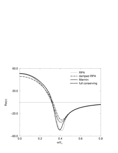
Figure 1: Plot of ${\mathrm{R}e}(\epsilon)$ against $\omega/E_{F}$ for a three-dimensional system. The parameters are $r_{s}=3$, $q=(0.2)k_{F}^{(3d)}$, $\tau=16/E_{F}^{(3d)}$ and $T=0.01E_{F}/k_{B}$.

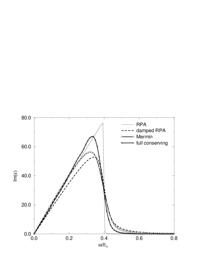
Figure 2: Plot of ${\mathrm{I}m}(\epsilon)$ against $\omega/E_{F}$ for a three-dimensional system. The parameters are the same as in Fig. 1.

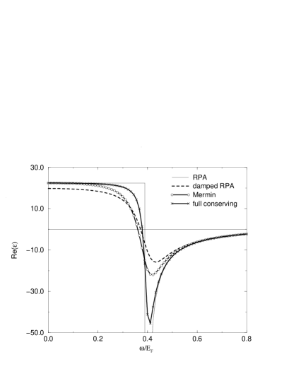
Figure 3: Plot of ${\mathrm{R}e}(\epsilon)$ against $\omega/E_{F}$ for a two-dimensional system. The parameters are $r_{s}=3$, $q=(0.2)k_{F}^{(2d)}$, $\tau=10/E_{F}^{(2d)}$ and $T=0.01E_{F}/k_{B}$.

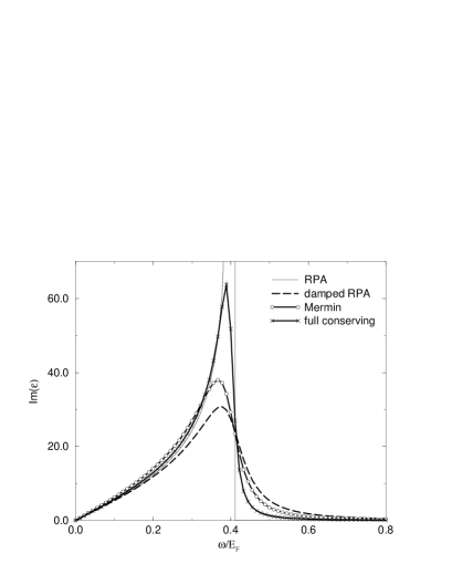
Figure 4: Plot of ${\mathrm{I}m}(\epsilon)$ against $\omega/E_{F}$ for a two-dimensional system. The parameters are the same as in Fig. 3.

Using the general form of the dielectric function as given by Eq. (27) we may immediately make comparisons with other prominent models proposed in the literature : (a) the undamped Lindhard DF (RPA) corresponding to the choices $E=0$, $F=0$ and $\tau\rightarrow\infty$, (b) the damped Lindhard DF: $E=0$, $F=0$ and finite $\tau$, (c) the Mermin DF : $E=0$, $F=[i/(\tilde{\omega}\tau)][1+C_{0}/B_{0}]$ and finite $\tau$, and finally (d) the FCDF given by Eq. (28), Eq. (29) and finite $\tau$. The real and imaginary parts of the various dielectric functions are shown for comparison in three dimensions (Fig. 1 and Fig. 2) and two dimensions (Fig. 3 and Fig. 4). It is not surprising that in all cases the behavior of the FCDF most closely resembles the RPA as it is only in these models that all the conservation laws are enforced.

III.2 Plasmon Dispersion

A simple application of any proposed DF is to determine the dispersion relationship, $\omega(q)$, of bulk longitudinal plasmons by imposing the condition : $\epsilon(q,\omega)=0$. Plasmon dispersion data can be obtained by scattering experiments involving X-rays or electrons. The measured quantity in these experiments is the energy loss of the scatterer which is directly related to the imaginary part of the DF. For the FCDF in the long wavelength limit it can be shown that

$$\lim_{q\to 0}\mathrm{Im}(\epsilon^{-1})=\frac{\pi}{2}\omega_{p}\delta(\omega-\omega_{p}).$$ (35)

Hence plasmons are the only energy loss at $q=0$ and we have exact fulfillment of the long wavelength ”perfect screening” sum rule Pines :

$$\lim_{q\to 0}\int_{0}^{\infty}\frac{1}{\omega}\mathrm{Im}\epsilon_{l}^{-1}(q,\omega)d\omega=\frac{\pi}{2}.$$ (36)

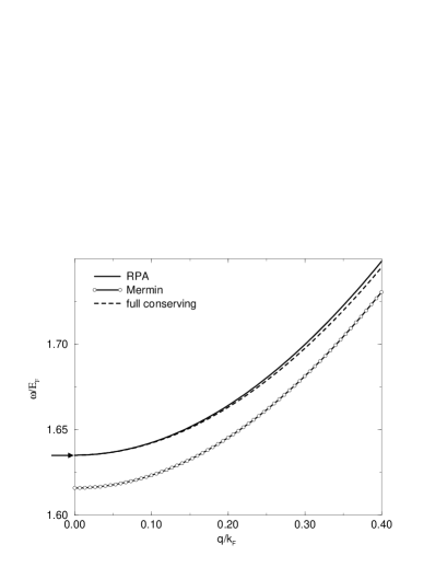
Figure 5: Three-dimensional plasmon dispersion. The parameters are $r_{s}=3$, $\tau=3/E_{F}^{(3d)}$ and $T=0.01E_{F}/k_{B}$. The arrow indicates the plasmon frequency, $\omega_{p}^{2}=4\pi e^{2}n_{0}/m$.

We analyze the solutions for plasmon dispersions arising from the various dielectric models as listed in the previous section. For three dimensions the differing models are compared in Fig. 5. As expected, the softening of the plasmon frequency from both the FCDF (at finite $q$) and the Mermin DF increases with $r_{s}$ and $1/\tau$. The salient differences between the models are exhibited in the limit $q\to 0$. The FCDF gives rise to the same plasmon energy gap, $\omega_{p}$, as the undamped Lindhard DF, as required from the sum rules for an electron liquid Pines . In Ref. Morawetz, the Mermin DF was apparently deduced to obey the perfect screening sum rule. However this claim can only be true in the limit $\omega\to\infty$ (or $\tau\to\infty$) and it must fail at finite $\omega$ as the 3D plasmon dispersion indicates. In fact, after a little algebra, it is possible to show that the Mermin DF gives rise to a Lorentzian spread in the energy loss,

$$\lim_{q\to 0}\mathrm{Im}(\epsilon_{\text{Mermin}}^{-1})=\frac{\omega_{p}^{2}\omega/\tau}{(\omega^{2}-\omega_{p}^{2})^{2}+(\omega/\tau)^{2}}.$$ (37)

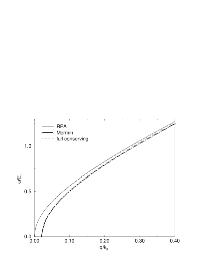
Figure 6: Two-dimensional plasmon dispersion. The parameters are $r_{s}=3$, $\tau=5/E_{F}^{(2d)}$ and $T=0.01E_{F}/k_{B}$.

The plasmon dispersion for two-dimensional systems is plotted in Fig. 6 where it should be noted that $\tau$ is assumed to be large enough such that localisation effects are negligible. As in the three-dimensional case, the plasma excitations from the Mermin DF and the FCDF are slightly softened with respect to the plasmon from RPA. Interestingly, the Mermin DF predicts a wavevector cuttoff below which a plasma mode cannot exist. This cutoff, which increases with $r_{s}$ and $1/\tau$, has also been previously noted Giuliani via the summation of ladder diagrams in the disorderd polarazibility function. The $q\to 0$ limit of the FCDF matches that of the RPA DF in agreement with the aforementioned sum rule. For comparable values of $r_{s}$ and $\tau$ the FCDF shows a greater deviation away from the RPA DF in two dimensions than in three. Clearly, scattering processes are less important for the three-dimensional plasmon because of the large frequency gap.

The damping of the two-dimensional plasmon, either from the presence of external impurities (Mermin DF) or electron-electron scattering (FCDF), occurs before the onset of Landau damping (not shown in figure) and thus may be amenable to experimental verification. In fact it has already been appreciated that experimental studies of two-dimensional electron systems are an important test of theoretical treatments of many-body effects (beyond RPA) which have been shown to be more important in two dimensions than in three Giuliani ; Jonson .

III.3 Conductivity

In a one-component system, and in an approximation where momentum is rigorously conserved, we expect a steady state D.C. current to increase indefinitely upon application of a constant external field. It can easily be shown that the conductivity, $\sigma$, as determined by the FCDF, is indeed infinite for the full-conserving model. To accommodate loss of momentum, thus rendering a finite conductivity, we return to the equation of motion

$$\langle{\bf p}\!+\!\frac{1}{2}{\bf q}|\widehat{\delta\rho}|{\bf p}\!-\!\frac{1}{2}{\bf q}\rangle(\omega-{\bf p}\cdot{\bf q}/m)+\Delta fU({\bf q})=-\frac{i}{\tau}\langle{\bf p}\!+\!\frac{1}{2}{\bf q}|\widehat{\rho}-\widehat{\rho}_{\text{loc}}|{\bf p}\!-\!\frac{1}{2}{\bf q}\rangle,$$ (38)

and impose static ($\omega\to 0$) and homogeneous (${\bf q}\to 0$) conditions, giving (in real space),

$$\delta{\bf j}=\delta{\bf j}_{\text{loc}}-n_{0}\tau\nabla U,$$ (39)

where

$$\delta{\bf j}_{\text{loc}}=\frac{2}{(2\pi)^{d}}\int d^{d}\!p\,e^{i({\bf q}\cdot{\bf r}-\omega\tau)}\langle{\bf p}\!+\!\frac{1}{2}{\bf q}|\widehat{\rho}_{\text{loc}}-\widehat{\rho}_{0}|{\bf p}\!-\!\frac{1}{2}{\bf q}\rangle{\bf p}.$$ (40)

If a fraction, $\lambda$, of the momentum density is conserved during collisions, i.e.

$$\delta{\bf j}_{\text{loc}}=\lambda\delta{\bf j},$$ (41)

then, using $e^{2}\delta{\bf j}/m=-\sigma\nabla U$, we obtain the familiar Drude conductivity

$$\sigma=n_{0}e^{2}\tau_{\text{m}}/m,$$ (42)

where we have defined an effective momentum-relaxation time,

$$\tau_{\text{m}}=\tau/(1-\lambda).$$ (43)

As expected, the conductivity diverges in the conserving limit, $\lambda\to 1$. In the presence of external scatterers (e.g. fixed impurities or Umklapp scattering), the other limit, $\lambda\to 0$, corresponds to isotropic scattering whereby the net momentum density is totally destroyed during collisions, and intermediate values of $\lambda$ reflect the degree of anisotropic scattering.

We may also include a second contribution to the collision integral stemming from additional scattering processes. These may include inelastic processes which we have up until now ignored. In other words, the relevant conductivity relaxation time, $\tau_{\text{cond}}$, may contain a contribution from both $\tau$ and an often larger energy relaxation time Mahan , $\tau^{\prime}$. To demonstrate this we assume, but without any strict justification, a (decoupled) relaxation time approximation for the inelastic contribution to the collision integral,

$$\left(\frac{\partial{\rho}}{\partial{t}}\right)_{\rm coll}=-\frac{(\widehat{\rho}-\widehat{\rho}_{\text{loc}})}{\tau}-\frac{(\widehat{\rho}-\widehat{\rho}_{\text{loc}}^{\prime})}{\tau^{\prime}},$$ (44)

where $\rho_{\text{loc}}^{\prime}$ describes a state of local equilibrium where all energy and momentum from the motion of particles has been lost. The expression for the conductivity then becomes,

$$\sigma=n_{0}e^{2}\tau_{\text{cond}}/m,$$ (45)

where $\tau_{\rm cond}^{-1}=\tau^{-1}_{\text{m}}+\tau^{\prime-1}_{\text{m}^{\prime}}$ (i.e. Matthiessen’s rule).

IV Semi-Classical Limit

We will now derive the dielectric function in a fully classical formalism except that at the end of the calculations we will still be free to employ a distribution appropriate for either a classical or a fermionic gas. The emerging result for the degenerate fermionic electron gas, whose equilibrium distribution is governed by quantum statistics, will be what we call the semi-classical limit.

The central dynamic quantity in classical transport theory is the phase space electron distribution $f({\bf p},{\bf r},t)$ governed by the Boltzmann equation. In the presence of an electric field, ${\bf E}$, the equation of motion in the relaxation time approximation is given by

$$\frac{\partial{f}}{\partial{t}}+\frac{\bf p}{m}\cdot\frac{\partial{f}}{\partial{\bf r}}+e{\bf E}\cdot\frac{\partial{f}}{\partial{\bf p}}=-\frac{f-f_{\rm loc}}{\tau}.$$ (46)

Magnetic effects are of second order and so disappear when the equation of motion is linearized. The total electric force, $e{\bf E}=-\nabla U$, has a contribution from an external source and an internal contribution from the induced charge density perturbation, as discussed in the quantum case. To determine the time development we now assume that the distribution function is slightly perturbed from equilibrium, and write

$$f({\bf p},{\bf r},t)=f_{0}({\bf p})+\delta f({\bf p},{\bf r},t).$$ (47)

As in the quantum case we work within the grand canonical ensemble which serves to define the global macroscopic temperature and chemical potential. To satisfy the local conservation laws, the local equilibrium distribution must be different from the global equilibrium distribution, $f_{0}$, and to first order is given by

$$f_{\rm loc}=f_{0}+\frac{\partial{f_{0}}}{\partial{\mu}}\delta\mu+\frac{\partial{f_{0}}}{\partial{\bf v}}\cdot\delta{\bf v}+\frac{\partial{f_{0}}}{\partial{T}}\delta T,$$ (48)

where

$${\bf v}=\int d^{d}\!p\frac{{\bf p}}{m}f.$$ (49)

Again, in our model we assume that the electrons have no initial drift velocity and only experience a net drift upon application of an electric field. Rewriting the local distribution as

$$f_{\rm loc}=f_{0}+\frac{\partial{f_{0}}}{\partial{\epsilon}}\delta\mu+\frac{\partial{f_{0}}}{\partial{\epsilon}}{\bf p}\cdot\delta{\bf v}+\frac{\partial{f_{0}}}{\partial{\epsilon}}\frac{(\epsilon-\mu)}{T}\delta T,$$ (50)

makes it transparent that it is indeed just the diagonal element of the corresponding quantum statistical operator in the limit ${\bf q}\rightarrow 0$. The Boltzmann transport equation, Eq. (46), now assumes the following form when linearized,

$$\frac{\partial{\delta f}}{\partial{t}}+\frac{\bf p}{m}\cdot\frac{\partial{\delta f}}{\partial{\bf r}}+e{\bf E}\cdot\frac{\partial{f_{0}}}{\partial{\bf p}}=-\frac{\delta f}{\tau}+\frac{1}{\tau}\frac{\partial{f_{0}}}{\partial{\epsilon}}\left[\delta\mu+{\bf p}\cdot\delta{\bf v}+\frac{(\epsilon-\mu)}{T}\delta T\right].$$ (51)

As in Sec. II.3 we now examine the consequences of applying the conservation laws. The terms $\delta\mu,\delta{\bf v},$ and $\delta T$ are independent of the electron momentum and must be determined by the local conservation laws for the collision invariants : average number, momentum and energy, i.e.

$$\int{d^{d}\!p}(f-f_{\rm loc})\left\{\begin{array}[]{cl}1\\ {\bf p}\\ p^{2}/2m\end{array}\right\}=\displaystyle\left\{\begin{array}[]{cl}0\\ 0\\ 0\end{array}\right\}.$$ (52)

Proceeding in a manner similar to that described in section II, the solutions are,

$$\delta\mu({\bf q},\omega)=\frac{\left(\displaystyle B^{\prime}_{0}2m\mu-B^{\prime}_{2}\right)\left(\displaystyle\frac{i\omega C^{\prime}_{2}}{\tau q^{2}n_{0}}\delta n+UC^{\prime}_{2}\right)+\delta n\left(D^{\prime}_{2}2m\mu-D^{\prime}_{4}\right)}{D^{\prime}_{4}B^{\prime}_{0}-D^{\prime}_{2}B^{\prime}_{2}},$$ (53)

$$\delta{\bf v}({\bf q},\omega)=\delta n\frac{\omega}{n_{0}q^{2}}{\bf q},$$ (54)

and

$$\delta T({\bf q},\omega)=2mT\frac{\delta n\left(D^{\prime}_{2}+\displaystyle\frac{i\omega B^{\prime}_{0}C^{\prime}_{2}}{q^{2}n_{0}}\right)+UC^{\prime}_{2}B^{\prime}_{0}}{D^{\prime}_{4}B^{\prime}_{0}-D^{\prime}_{2}B^{\prime}_{2}}.$$ (55)

We have introduced the classical versions of the integral functions defined in section II, i.e.

$$B^{\prime}_{n}=\frac{2}{(2\pi)^{d}}\int d^{d}p|{\bf p}|^{n}\frac{\partial{f_{0}}}{\partial{\epsilon}},$$ (56)

$$C^{\prime}_{n}=\frac{2}{(2\pi)^{d}}\int d^{d}p|{\bf p}|^{n}\frac{\partial{f_{0}}}{\partial{\bf p}}\cdot{\bf q}\frac{1}{\tilde{\omega}-{\bf p}\cdot{\bf q}/m},$$ (57)

and

$$D^{\prime}_{n}=\frac{C^{\prime}_{n}+i\omega\tau B^{\prime}_{n}}{i\tilde{\omega}\tau}.$$ (58)

Note that the expressions for the thermodynamic variations also differ from their quantum counterparts in that terms of order $q^{2}$ are absent.

We can now obtain the dielectric response of the system with a treatment similar to that given above. The DF that follows from solving for $\delta n$ in the transport equation is identical to Eq. (27) except that the integral functions, $B_{n}$, $C_{n}$ and $D_{n}$ are replaced by their classical counterparts, $B^{\prime}_{n}$, $C^{\prime}_{n}$ and $D^{\prime}_{n}$. The interesting point here is that functional form is therefore preserved in both the quantum result and in the classical approximation. Interestingly, an early attempt to ”guess” a quantum number-conserving response from the classical response led to erroneous results Kliewer . However the work presented in this paper suggests that the the correct response may be correctly guessed from the classical response but only if the classical response can be written in terms of macroscopic moments of the Lindhard polarizability function.

The semi-classical result follows by taking $f_{0}$ to be the equilibrium fermionic distribution. In this case the integral functions, $B^{\prime}_{n}$, $C^{\prime}_{n}$ and $D^{\prime}_{n}$, and hence the semi-classical DF, represent the low $q$ expansion of their quantum (unprimed) counterparts in Sec. II.3 and Sec. III.1, respectively.

V Hydrodynamics of a degenerate electron gas

A hydrodynamic description is obtained by coarse-graining over the microscopic degrees of freedom in such a way that the dynamical equations are expressed in terms of macroscopic quantities only. The hydrodynamic equations are traditionally derived from the classical Boltzmann equation Eq. (46) and this indeed is the approach employed by Tokatly and Pankratov Tokatly1 who also recently formulated the hydrodynamic theory of an electron gas to arbitrary frequencies. Here we provide a derivation from the quantum description of the microscopic dynamics and begin by writing the macroscopic quantities in terms of the one-particle statistical operator,

$$n({\bf r},t)=\langle{\bf r}|\widehat{\rho}|{\bf r}\rangle,$$ (59)

$${\bf j}({\bf r},t)=mn({\bf r},t){\bf v}({\bf r},t)=\frac{1}{2}\langle{\bf r}|\{\widehat{\rho},\widehat{\bf p}\}|{\bf r}\rangle,$$ (60)

$$U({\bf r},t)=\langle{\bf r}|\widehat{U}|{\bf r}\rangle,$$ (61)

and

$$P_{ij}({\bf r},t)=\frac{1}{2m}\langle{\bf r}|\{\widehat{\rho},(\widehat{p_{i}}-mv_{i})(\widehat{p_{i}}-mv_{i})\}|{\bf r}\rangle,$$ (62)

where $\{,\}$ denotes symmetrization (i.e. anticommutation), $n$ and ${\bf j}$ can be shown to be equivalent to the definitions in Eq. (13), and $P_{ij}$ is the local stress tensor in the comoving frame. Higher momentum moments can be neglected in a second order theory of a degenerate electron gas, i.e. thermal effects are negligible since $k_{B}T\ll E_{F}$. The conserving constraints can also be expressed in a similar manner, namely

$$\langle{\bf r}|\widehat{\rho}-\widehat{\rho}_{\rm loc}|{\bf r}\rangle=0,$$ (63)

$$\langle{\bf r}|\{(\widehat{\rho}-\widehat{\rho}_{\rm loc}),\widehat{\bf p}\}|{\bf r}\rangle=0,$$ (64)

and

$$\langle{\bf r}|\{(\widehat{\rho}-\widehat{\rho}_{\rm loc}),\widehat{H}_{0}\}|{\bf r}\rangle=0.$$ (65)

The hydrodynamic equations follow by taking diagonal elements (in position representation) of the quantum dynamical equation, which we repeat here,

$$\frac{\partial{\widehat{\rho}}}{\partial{t}}+i\left[\left(\frac{\widehat{p}^{2}}{2m}+\widehat{U}\right),\widehat{\rho}\right]=\frac{\widehat{\rho}_{\rm loc}-\widehat{\rho}}{\tau},$$ (66)

but symmetrized with the relevant operators from each conservation law. Before proceeding we note than an alternative approach to deriving the equations of motion of thermodynamic coordinates from the quantum Liouville equation, but not necessarily close to equilibrium, has been discussed via the time-dependent projection operator technique Jaynes .

The first hydrodynamic equation, the equation of continuity, is simply obtained by taking the diagonal element of Eq. (66), eventually giving

$$\frac{Dn}{Dt}+n\nabla_{i}v_{i}=0,$$ (67)

where $D_{t}=\partial_{t}+v_{i}\nabla_{i}$ is the covariant derivative. The derivation requires use of the fact that for a one-body potential, $\langle{\bf r}|[\widehat{U},\widehat{\rho}]|{\bf r}\rangle=0$ and that $\langle{\bf r}|[\widehat{\bf p},\widehat{A}]|{\bf r}\rangle=i\nabla\langle{\bf r}|\widehat{A}|{\bf r}\rangle$ for any operator $\widehat{A}$. The next hydrodynamic equation follows by anticommuting Eq. (66) with $\widehat{\bf p}$ and then taking the diagonal element, culminating in

$$mn\frac{Dv_{i}}{Dt}+\nabla_{i}p+\nabla_{j}\pi_{ij}-n\nabla_{i}U=0,$$ (68)

where the symmetric stress tensor, $P_{ij}$, has been decomposed into scalar and traceless parts, i.e.

$$P_{ij}=p\delta_{ij}+\pi_{ij}$$ (69)

and

$${\rm{Tr}}\pi_{ij}=0.$$ (70)

The scalar $d$-dimensional pressure of the gas in local equilibrium is given by

$$p=\frac{1}{d}{\rm{Tr}}P_{ij}$$ (71)

which for an ideal and degenerate Fermi gas, of spin degeneracy $2$, can be calculated to be

$$p\equiv\frac{k_{B}T}{V}\ln{\mathcal{Z}}=\frac{2^{2-2/d}\pi[\Gamma(1+d/2)]^{2/d}}{d+2}\frac{n_{0}^{1+2/d}}{m}+O\left(\left(\frac{k_{B}T}{E_{F}}\right)^{2}\right),$$ (72)

where $\mathcal{Z}$ is the grand canonical partition function. The third hydrodynamic equation, obtained by anticommuting Eq. (66) with $\widehat{p_{i}}\widehat{p_{j}}$, is given to second order by

$$\frac{DP_{ij}}{Dt}+P_{ij}\nabla_{k}v_{k}+P_{ik}\nabla_{k}v_{j}+P_{kj}\nabla_{k}v_{i}=-\frac{\pi_{ij}}{\tau}.$$ (73)

By decomposing $P_{ij}$ into $p$, Eq. (72), and $\pi_{ij}$ we actually get two equations from Eq. (73), namely

$$\pi_{ik}\nabla_{k}v_{i}=0$$ (74)

and

$$\frac{D\pi_{ij}}{Dt}+\pi_{ij}\nabla_{k}v_{k}+\pi_{ik}\nabla_{k}v_{j}+\pi_{kj}\nabla_{k}v_{i}-\frac{2}{d}\delta_{ij}\pi_{\mu k}\nabla_{k}v_{\mu}+p\left(\nabla_{i}v_{j}+\nabla_{j}v_{i}-\frac{2}{d}\delta_{ij}\nabla_{k}v_{k}\right)=-\frac{\pi_{ij}}{\tau}.$$ (75)

The complete set of hydrodynamical equations is then specified by Eq. (67), Eq. (68), Eq. (72), Eq. (74) and Eq. (75). Traditional Bloch (adiabatic) hydrodynamics is recovered by setting $\pi_{ij}=0$. The presence of $\pi_{ij}$ stems from the anisotropy of the stress tensor, i.e. the inability of the dynamic electron gas to achieve local equilibrium. The content of Eq. (75) shows that the extent of anisotropic dynamics are tempered by relaxation effects which drive the system back to an isotropic state of local equilibrium.

We now demonstrate the efficacy of these equations in correcting the shortcomings of the traditional adiabatic hydrodynamics in predicting the longitudinal plasmon dispersion. The simplest route to calculating the dispersion of the collective mode, in say the $x$ direction, is to first linearize the hydrodynamic equations, giving

$$\frac{\partial{\delta n}}{\partial{t}}+n_{0}\nabla_{x}v_{x}=0,$$ (76)

$$mn_{0}\frac{\partial{v_{x}}}{\partial{t}}+\nabla_{x}\delta p+\nabla_{x}\delta\pi_{xx}-n_{0}\nabla_{x}U=0,$$ (77)

$$\delta p=\frac{(d+2)}{d}\frac{p_{0}}{n_{0}}\delta n,$$ (78)

and

$$\frac{\partial{\delta\pi_{xx}}}{\partial{t}}+\frac{2d-2}{d}p_{0}\nabla_{x}v_{x}=-\frac{\delta\pi_{xx}}{\tau},$$ (79)

and then to consider a plane-wave solution $e^{i(qx-\omega t)}$ in the absence of an external field, i.e. $U=U_{\rm int}$. Ignoring retardation effects, the potential energy $U({\bf r},t)$ is simply the convolution of the density perturbation and the Coulomb potential energy, which can be expressed in Fourier space as $U(q)=-\delta n(q)V(q)$, i.e. mean-field Hartree potential. Solving the linearized equations then gives the following solution,

$$\omega^{2}=\omega_{p}^{2}(q)+\beta^{2}(\omega)q^{2},$$ (80)

where $\omega_{p}(q)$ is given by Eq. (34) and

$$\beta^{2}(\omega)=\left[\frac{d+2}{d}+\frac{2d-2}{d}\left(\frac{\omega}{\tilde{\omega}}\right)\right]\frac{p_{0}}{mn_{0}},$$ (81)

or

$$\beta(\omega)=\left[\frac{1}{d}+\frac{2d-2}{d(d+2)}\left(\frac{\omega}{\tilde{\omega}}\right)\right]^{1/2}v_{F}.$$ (82)

The coefficient $\beta$ interpolates between the correct limiting forms of both the hydrodynamic regime ($\omega\tau\ll 1$), in agreement with conventional adiabatic hydrodynamic theory, and the collisionless regime ($\omega\tau\gg 1$), in agreement with RPA RPAexplain . In a $d$-dimensional electron gas, the low frequency limit entails the fact that collisions are effective in maintaining a local equilibrium and thus a conduction electron possesses $d$ translational degrees of freedom. In the opposite high-frequency limit the influence of collisions is negligible and the electron has effectively one translational degree of freedom, corresponding to motion in the direction of the applied field. The notion of effective number of degrees of freedom, $f$, can be made quantitative by comparing Eq. (81) with the same result in the adiabatic limit, i.e. ignoring the second term in brackets, giving

$$f(\omega)=\frac{d\tilde{\omega}}{\tilde{\omega}+(d-1)\omega}.$$ (83)

The limiting forms of $f(\omega)$ and $\beta(\omega)$ may be summarized as

$$\begin{array}[]{l}f(\omega)=d,\\ \beta(\omega)=(1/d)^{1/2}v_{F},\end{array}\hskip 28.45274pt(\omega\tau\ll 1)$$ (84)

and

$$\begin{array}[]{l}f(\omega)=1,\\ \beta(\omega)=[3/(d+2)]^{1/2}v_{F}.\end{array}\hskip 28.45274pt(\omega\tau\gg 1)$$ (85)

In three dimensions, Eq. (82) and Eq. (83) agree with those derived by Halevi Halevi who determined the $\omega$-dependence of $\beta$ by comparing a (damped) hydrodynamic DF with the Mermin DF. The need for a frequency-dependent $\beta$ has also been noted in the context of a hydrodynamic description of inhomogeneous electron systems Dobson . The cross-over between the collisional and collisionless regime has also recently been discussed in an interesting paper elastic discussing the viscoelastic behavior of an electron liquid.

Finally, we note that a popular way of implementing phenomenological damping in hydrodynamic models of an electron gas through the use of Fetter

$$\frac{Dn}{Dt}+n\nabla_{i}v_{i}=0,$$ (86)

and

$$m\frac{Dv_{i}}{Dt}+\frac{\nabla_{i}P}{n}-\nabla_{i}U=-m\frac{v_{i}}{\tau},$$ (87)

is simply the hydrodynamic approximation of the Mermin model in the adiabatic regime and where all momentum is destroyed during collisions, i.e. Eq. (86) and Eq. (87) are obtained from Eq. (66) with the following constraints, namely

$$\langle{\bf r}|\widehat{\rho}-\widehat{\rho}_{\rm loc}|{\bf r}\rangle=0,$$ (88)

$$\pi_{ij}=0,$$ (89)

and

$$\langle{\bf r}|\{\widehat{\rho}_{\rm loc},\widehat{\bf p}\}|{\bf r}\rangle=0.$$ (90)

VI Conclusion

The relaxation-time approximation has been applied to the quantum dynamics of a $d$-dimensional electron gas where (average) number, momentum and energy are conserved during collisions. It has been shown that the requirement of conservation of all collision invariants necessitates a state of local equilibrium, to which the electrons relax, with a space- and time-dependent chemical potential, drift velocity and temperature. The ensuing dielectric response has been determined and compared with others in the literature, revealing that, in general, that imposition of the conservation laws tends to make the dielectric response in the relaxation-time approximation more akin to the RPA dielectric response than without them. The FCDF attains the correct static limit and obeys the perfect screening sum rule.

The resultant plasmon dispersion has been compared with others and relaxation has been shown to induce softening of the plasmon with increasing $r_{S}$ and $1/\tau$. In both three and two dimensions and in the long wavelength limit, the plasmon dispersion from FCDF is in good agreement with that derived from the RPA. In general, correlation effects are more pronounced in two dimensions than in three and thus further experimental study of two-dimensional plasmons ought to provide a significant test of models of dynamical correlation.

The derivation of the conserving reponse has been repeated but in a semi-classical formalism using the Boltzmann transport equation. The functional form of the ensuing response is then identical to that obtained by quantum kinetic arguments.

The hydrodynamic equations of a degenerate electron gas are derived from the quantum microscopic equation of motion using the relaxation time approximation and fulfillment of all the conservation laws. The departure of the stress tensor from a scalar is due to inertial effects but counteracted by relaxation effects. The competition between these two effects gives rise to a generalization of the hydrodynamics applicable to all frequencies and thus correctly reproduces the collision-dominated adiabatic limit ($\omega\tau\ll 1$) and the collisionless limit ($\omega\tau\gg 1$).

Given that the FCDF aims to incorporate dynamic electron correlation effects via a phenomenological $\tau$ it is interesting to compare this with dielectric funtions which include correlation effects via a many-body field-theoretic approach giving rise to dynamic local field factors Singwi . In principle the two different approaches ought to exhibit the same qualitative behavior (with respect to differences from the RPA) and indeed this is what we observe. In this context we can view the relaxation-time approximation as being a crude way of including Feynman diagrams beyond the RPA in the proper polarizability of an electron liquid. To extend the comparisons in a more quantitative and direct manner further work is required, i.e. calculation of an expression for $\tau$ and inclusion of exchange in the FCDF.

Finally, we repeat here that the analysis in this paper explicitly calculates the response function only when all the conservation laws are obeyed, as required for a one-component system, but, using the results of Appendix C, the response functions can be calculated which obey fewer and in different combinations. This is the case required in, for example, two-component systems or when crystalline effects are incorporated by way of Umklapp scattering.

VII Acknowledgements

This work was supported by the National Science Foundation under grant number DMR-9988576. We thank Prof. B. Tanatar for bringing some recent literature to our attention.

Appendix A Thermodynamics of a local equilibrium state

In this appendix we elaborate on what is meant by local values of $\mu$, ${\bf v}$ and $T$, in the thermodynamic sense.

We first recall how temperature and chemical potential are defined for a large (macroscopic) system, A, lying in contact with a heat reservoir, B, with which it can exchange particles and energy. Thermodynamic equilibrium of the system+reservior setup is achieved when the entire entropy of the system+reservoir is maximized,

$$\left(\frac{\partial{S_{A+B}}}{\partial{U_{A}}}\right)_{N,V}=\left(\frac{\partial{S_{A+B}}}{\partial{N_{A}}}\right)_{U,V}=0$$ (91)

From the conservation of total particle number, energy and volume we arrive at the equality of three thermodynamic variables which we identify as the temperature ($T_{A}=T_{B}$) and the chemical potential ($\mu_{A}=\mu_{B}$). Throughout the system $\mu$ and $T$ are constants independent of space and time. By appealing to the strong Coulomb attraction between the electrons and the positive background we can infer that the velocity field, ${\bf v}_{A}$, and hence the pressure, is also constant throughout. The constant nature of the thermodynamic variables is due to the effect of relaxation processes which drive the system towards equilibrium. Now, if the system is perturbed slightly, these variables may attain a spatial variation and will still remain thermodynamically well-defined if the subsection of the system over which they vary slightly is much greater than the average distance between collisions. Thus we require that

$$|{\bf q}|l_{\text{mf}}\ll 1,$$ (92)

where ${\bf q}$ is the wavevector of the spatial fluctuations of $\mu$, ${\bf v}$ and $T$, and $l_{\text{mf}}$ is the mean free path which can be approximated as $v_{F}\tau$. In addition the time variation of the thermodynamic variables must be slower than the relaxation time scale in order for the relaxation processes to maintain the state of local equilibrium, i.e.

$$\omega\tau\ll 1.$$ (93)

This constraint is consistent with the fact that the scattering term, and hence the presence of $f_{\rm loc}$ only becomes important in the limit that $\tau$ is small.

These considerations suggest that the local equilibrium state may be an adiabatic one and indeed we can show that $f_{\rm loc}$ is a small perturbation away from $f_{0}$ such that there is no entropy production. We begin by recalling the Von Neumann definition of entropy,

$$S=-k_{B}\rm{Tr}(\widehat{\rho}_{\rm gc}\ln\widehat{\rho}_{\rm gc}),$$ (94)

where the trace is carried out over all possible microstates in the grand canonical ensemble and $\rho_{\rm gc}$ is the statistical operator of the grand canonical ensemble. This expression can be written in terms of the one-particle fermionic statistical operator, $\widehat{\rho}$, Thirring

$$S=-k_{B}\rm{tr}[\widehat{\rho}\ln\widehat{\rho}+(1-\widehat{\rho})\rm ln(1-\widehat{\rho})],$$ (95)

where $tr$ denotes the trace over one-particle states. In a non-equilibrium distribution the occupation and distribution of states acquire both a spatial and time dependence and thus, in general, the entropy will be a function of time. The time variation of $\widehat{\rho}_{\rm loc}$ is determined by substitution into Eq. (66) giving

$$\frac{\partial{\widehat{\rho}_{\rm loc}}}{\partial{t}}=-i[\widehat{H},\widehat{\rho}_{\rm loc}],$$ (96)

and it follows that when $\widehat{\rho}=\widehat{\rho}_{\rm loc}$

$$\frac{\partial{S}}{\partial{t}}=0.$$ (97)

We note that this derivation is essentially the quantum analogue of Boltzmann’s $\Theta$ (or $\mathcal{H}$)-theorem. Thus the variations of $\mu$, ${\bf v}$ and $T$, that characterize the local equilibrium state, are constrained to prevent the production of entropy in the system. The situation is identical to the propagation of sound in an Euler fluid or first sound in superfluid Helium II (to lowest order in $(\delta n/\delta T)_{P}$): a linearized disturbance away from equilibrium gives rise to an isentropic (constant entropy density) longitudinal traveling wave with local variations in density, pressure and temperature.

Appendix B Useful Integrals

The integrals defined in this paper can be expressed as moments of the polarizability function, $\chi$, in the Lindhard dielectric constant. The Lindhard polarizability, in $d$ dimensions, is given by

$$\chi({\bf q},\omega)=\frac{2}{(2\pi)^{d}}\int d^{d}\!p\,\frac{f_{{\bf p}+\frac{1}{2}{\bf q}}-f_{{\bf p}-\frac{1}{2}{\bf q}}}{\omega-{\bf p}\cdot{\bf q}/m+i0^{+}}.$$ (98)

We now define the $n-$th momentum moment of the polarizability function as

$$\chi_{n}({\bf q},\omega)=\frac{2}{(2\pi)^{d}}\int d^{d}\!p\,|{\bf p}|^{n}\frac{f_{{\bf p}+\frac{1}{2}{\bf q}}-f_{{\bf p}-\frac{1}{2}{\bf q}}}{\omega-{\bf p}\cdot{\bf q}/m+i0^{+}}.$$ (99)

Here we demonstrate how analytical expressions may be obtained in the low q limit for a degenerate electron gas. In this limit,

$${\mathrm{Re}}\chi_{n}({\bf q},\omega) = \frac{2}{(2\pi)^{d}}{\mathcal{P}}\int d^{d}\!p\,\frac{\partial{f}}{\partial{\epsilon}}\,\frac{|{\bf p}|^{n}\,{\bf p}\cdot{\bf q}}{\omega m-{\bf p}\cdot{\bf q}},$$ (100)

$${\mathrm{Im}}\chi_{(}{\bf q},\omega) = \frac{1}{(2\pi)^{d-1}}\int d^{d}\!p\frac{\partial{f}}{\partial{\epsilon}}|{\bf p}|^{n}{\bf p}\cdot{\bf q}\,\delta(\omega m-{\bf p}\cdot{\bf q}).$$ (101)

In spherical coordinates the real part becomes,

$${\mathrm{Re}}\chi_{n}({\bf q},\omega) = \frac{2m\Omega_{d-1}}{q(2\pi)^{d}}\,{\mathcal{P}}\!\int dp\,\frac{\partial{f}}{\partial{\epsilon}}p^{d-2+n}\int_{0}^{\pi}d\phi\left(\omega I[\phi,p]-\frac{pq}{m}\sin^{d-2}\!\phi\right),$$ (102)

$$I[\phi,p] = \frac{\sin^{d-2}\!\phi}{\frac{\omega m}{pq}-\cos\phi},$$

where $\Omega_{d}=2\pi^{d/2}/\Gamma(d/2)$ is the surface area of a unit d-dimensional sphere. Upon elementary transformations and exploiting the integral representation of the hypergeometric function,

$$F(a,b,c;z)=\frac{\Gamma(c)}{\Gamma(b)\Gamma(c-b)}\int_{0}^{1}dt\,t^{b-1}(1-t)^{c-b-1}(1-tz)^{-a},\hskip 28.45274pt(c>b>0),$$ (103)

it is possible to obtain

$$\int_{0}^{\pi}d\phi I[\phi,p]=\left\{\begin{array}[]{l}\displaystyle\frac{{\sqrt{\pi}\,\Gamma(\frac{d-1}{2})}}{{\Gamma(d/2)}}\left(\frac{p\,q}{\omega m}\right)F\left[1,\frac{1}{2},\frac{d}{2};\left(\frac{p\,q}{\omega m}\right)^{2}\right]\hskip 56.9055pt(\omega m>p\,q)\\ \displaystyle\frac{{2\sqrt{\pi}\,\Gamma(\frac{d-1}{2})}}{{\Gamma(\frac{d}{2}-1)}}\left(\frac{\omega m}{p\,q}\right)F\left[1,2-\frac{d}{2},\frac{3}{2};\left(\frac{\omega m}{p\,q}\right)^{2}\right]\hskip 28.45274pt(p\,q>\omega m)\end{array}\right.$$ (104)

and

$$\int_{0}^{\pi}d\phi\,\sin^{d-2}\!\phi=\displaystyle\frac{{\sqrt{\pi}\Gamma(\frac{d-1}{2})}}{{\Gamma(d/2)}}.$$ (105)

If we assume, as is the case for a degenerate electron gas, that $k_{B}T$ is much lower than the Fermi energy then the momentum integral can be simplified with the substitution $\frac{\partial{f}}{\partial{\epsilon}}=-\delta(\epsilon-\epsilon_{F})$. The final expressions, at this low temperature, are then,

$$\rm{Re}\chi_{n}({\bf q},\omega)=\left\{\begin{array}[]{ll}\displaystyle\frac{{m2^{2-d}p_{F}^{d-2+n}}}{{\pi^{d/2}\Gamma(d/2)}}\left\{1-F\left[1,\frac{1}{2},\frac{d}{2};\left(\frac{p_{F}q}{\omega m}\right)^{2}\right]\right\}&(\omega m>p_{F}q)\\ \displaystyle\frac{{m2^{2-d}p_{F}^{d-2+n}}}{{\pi^{d/2}\Gamma(d/2)}}\left\{1-\displaystyle\frac{{2\Gamma(d/2)}}{{\Gamma(-1+d/2)}}\left(\frac{\omega m}{p_{F}q}\right)^{2}F\left[1,2-\frac{d}{2},\frac{3}{2};\left(\frac{\omega m}{p_{F}q}\right)^{2}\right]\right\}&(p_{F}q>\omega m).\end{array}\right.$$ (106)

The static limit of $\rm{Re}\chi_{n}$ is thus identified with the function, $B_{n}({\bf q})$, for a highly degenerate electron gas.

Appendix C Generalised solution for thermodynamic fluctuations

The macroscopic fluctuations of $\delta n$, $\delta{\bf J}$ and $\delta E$, as defined by Eq. (12), can be obtained by taking the relevant momentum moments of the microscopic equation of motion which we rewrite here in terms of ${\bf q}$,

$$(\omega-\Delta\epsilon)\langle{\bf p}\!+\!\frac{1}{2}{\bf q}|\widehat{\delta\rho}|{\bf p}\!-\!\frac{1}{2}{\bf q}\rangle+\Delta fU({\bf q})=-\frac{i}{\tau}\left(\langle{\bf p}\!+\!\frac{1}{2}{\bf q}|\widehat{\delta\rho}|{\bf p}\!-\!\frac{1}{2}{\bf q}\rangle\!+\!\frac{\Delta f}{\Delta\epsilon}\left[\delta\mu({\bf q})+{\bf p}\cdot\delta{\bf v}({\bf q})+(\frac{p^{2}}{m}+\frac{q^{2}}{2m}-\mu)\displaystyle\frac{\delta T({\bf q})}{T}\right]\right).$$ (107)

However, since we assert that the macroscopic quantities are conserved before and after each collision, we must obtain two sets of expressions for each term. The first set, determined by the dynamics after each collision process (i.e. right-hand side of Eq. (107)) is given by Eq. (12). The second set follows from solving the entire microscopic equation, Eq. (107), for $\langle{\bf p}\!+\!\frac{1}{2}{\bf q}|\widehat{\delta\rho}|{\bf p}\!-\!\frac{1}{2}{\bf q}\rangle$ and then taking moments, i.e.

$$\left(\begin{array}[]{c}\delta n\\ \delta{\bf j}\\ \delta E\end{array}\right)=-U({\bf q})\left(\begin{array}[]{c}P[\Delta\epsilon]\\ P[{\bf p}\Delta\epsilon]\\ P[\frac{p^{2}}{2m}\Delta\epsilon]\end{array}\right)-\frac{i}{\tau}\left(\begin{array}[]{c}P[\delta\mu({\bf q})+{\bf p}\cdot\delta{\bf v}({\bf q})+(\frac{p^{2}}{m}+\frac{q^{2}}{2m}-\mu)\displaystyle\frac{\delta T({\bf q})}{T}]\\ P[{\bf p}(\delta\mu({\bf q})+{\bf p}\cdot\delta{\bf v}({\bf q})+(\frac{p^{2}}{m}+\frac{q^{2}}{2m}-\mu)\displaystyle\frac{\delta T({\bf q})}{T})]\\ P[\frac{p^{2}}{2m}(\delta\mu({\bf q})+{\bf p}\cdot\delta{\bf v}({\bf q})+(\frac{p^{2}}{m}+\frac{q^{2}}{2m}-\mu)\displaystyle\frac{\delta T({\bf q})}{T})]\end{array}\right),$$ (108)

where

$$P[g]=\frac{2}{(2\pi)^{d}}\int d^{d}\!p\,\frac{\Delta f}{\Delta\epsilon}\,\frac{g}{\tilde{\omega}-\Delta\epsilon}.$$ (109)

Upon expansion of partial fractions we can obtain

$$\left(\begin{array}[]{c}\delta n\\ \delta{\bf j}\cdot{\bf q}\\ \delta E\end{array}\right)=-U({\bf q})\left(\begin{array}[]{c}C_{0}\\ \tilde{\omega}C_{0}\\ \frac{C_{2}}{2m}\end{array}\right)+\frac{1}{i\tilde{\omega}\tau}\left(\begin{array}[]{lll}B_{0}+C_{0}&C_{0}\frac{\tilde{\omega}}{q^{2}}&\frac{B_{2}+C_{2}}{2m}+(\frac{q^{2}}{8m}-\mu)(B_{0}+C_{0})\\ C_{0}\tilde{\omega}&C_{0}\frac{{\tilde{\omega}}^{2}}{q^{2}}&\frac{C_{2}}{2m}\tilde{\omega}+(\frac{q^{2}}{8m}-\mu)C_{0}\tilde{\omega}\\ \frac{B_{2}+C_{2}}{2m}&\frac{C_{2}}{2m}\frac{\tilde{\omega}}{q^{2}}&\frac{B_{4}+C_{4}}{4m^{2}}+(\frac{q^{2}}{8m}-\mu)\frac{B_{2}+C_{2}}{2m}\end{array}\right)\left(\begin{array}[]{c}\delta\mu\\ \delta{\bf v}\cdot{\bf q}\\ \frac{\delta T}{T}\end{array}\right),$$ (110)

where we have, for convenience, taken the component of momentum density along q. In addition we have assumed that the direction of the momentum density lies entirely in the q direction, a property that fails for Non-Newtonian fluids. With this expression, together with Eq. (12), it is possible to eliminate the conserved quantities to solve for the thermodynamic variations,

$$\left(\begin{array}[]{ccc}D_{0}&\frac{C_{0}}{q^{2}i\tau}&\frac{D_{2}}{2m}+(\frac{q^{2}}{8m}-\mu)D_{0}\\ \frac{C_{0}}{i\tau}&\frac{\tilde{\omega}C_{0}}{i\tau q^{2}}-n_{0}&\frac{C_{2}}{2mi\tau}+(\frac{q^{2}}{8m}-\mu)\frac{C_{0}}{i\tau}\\ \frac{D_{2}}{2m}&\frac{C_{2}}{2mq^{2}i\tau}&\frac{D_{4}}{4m^{2}}+(\frac{q^{2}}{8m}-\mu)\frac{D_{2}}{2m}\end{array}\right)\left(\begin{array}[]{c}\delta\mu\\ \delta{\bf v}\cdot{\bf q}\\ \frac{\delta T}{T}\end{array}\right)=U({\bf q})\left(\begin{array}[]{c}C_{0}\\ \tilde{\omega}C_{0}\\ \frac{C_{2}}{2m}\end{array}\right).$$ (111)

References

- (1) J. Lindhard, Kgl. Danske Videnskab. Selskab, Mat.-Fys. Medd 28 8 (1954).
- (2) N. D. Mermin , Phys. Rev. B 1, 2362 (1970).
- (3) P. Garik and N. W. Ashcroft, Phys. Rev. B 21, 391 (1980).
- (4) D. M. Wood and N. W. Ashcroft, Phys. Rev. B 25, 6255 (1982).
- (5) A. Selchow and K. Morawetz, Phys. Rev. E 59, 1015 (1999).
- (6) G. Atwal and N. W. Ashcroft, Bull. Am. Phys. Soc. 45, 867 (2000); 46 1147 (2001).
- (7) K. Morawetz and U. Fuhrmann, Phys. Rev. E 61, 2272; 62, 4382 (2000); K. Morawetz cond-mat/0104229 (unpublished).
- (8) The term “conserving approximation” is also used in the Green’s function approach to transport theory, G. Baym and L. P. Kadanoff, Phys. Rev. 124, 287 (1961). Conservations laws are implemented there by defining a suitable approximation for the one-particle Green’s function.
- (9) F. Bloch, Z. Phys. 81, 363 (1933).
- (10) I. Tokatly and O. Pankratov, Phys. Rev. B 60, 15550 (1999), 62, 2759 (2000).
- (11) D. Pines and P. Nozieres, The Theory of Quantum Liquids, (W. A. Benjamin, New York, 1996).
- (12) G. F. Giuliani and J. J. Quinn, Phys. Rev. B 29, 2321 (1984).
- (13) M. Jonson, J. Phys. C 9, 3055 (1976).
- (14) G. D. Mahan, Many-particle physics Plenum Press, New York, (1990).
- (15) K. L. Kliewer and R. Fuchs, Phys. Rev. 181, 552 (1969).
- (16) E. T. Jaynes, Phys. Rev. 106, 620 (1957); B. Robertson, Phys. Rev. 144, 151 (1966); R. Balian, Y. Alhassid, and H. Reinhardt, Phys. Rep. 131, 2 (1986).
- (17) The oft-used statement that RPA is valid only in the collisionless regime is strictly inaccurate since, of course, the RPA does incorporate correlation effects via the mean-field potential (one-body operator) from Poisson’s equation. By collisionless we thus mean that the two-body operator term describing scattering process, the right-hand side of Eq. (3), is negligible.
- (18) P. Halevi, Phys. Rev. B 51, 7497 (1995).
- (19) J.F. Dobson and H.M. Le, Theo Chem 501, 327 (2000).
- (20) S. Conti and G. Vignale, Phys. Rev. B 60, 7966 (1999).
- (21) A. L. Fetter, Ann. Phys. (N.Y.) 81, 367 (1973).
- (22) A. Holas, P. K. Aravind, and K. S. Singwi, Phys. Rev. B 20, 4912 (1979); A. Czachor, A. Holas, S. R. Sharma, and K. S. Singwi, Phys. Rev. B 25, 2144 (1982).
- (23) W. Thirring, Quantum Mechanics of Large Systems, (Springer-Verlag, 1980).