Thermodynamics of self-gravitating systems

Abstract

We study the thermodynamics and the collapse of a self-gravitating gas of Brownian particles. We consider a high friction limit in order to simplify the problem. This results in the Smoluchowski-Poisson system. Below a critical energy or below a critical temperature, there is no equilibrium state and the system develops a self-similar collapse leading to a finite time singularity. In the microcanonical ensemble, this corresponds to a “gravothermal catastrophe” and in the canonical ensemble to an “isothermal collapse”. Self-similar solutions are investigated analytically and numerically.

1 Introduction

The thermodynamics of self-gravitating systems displays intriguing features due to the existence of negative specific heats, inequivalence of statistical ensembles and phase transitions associated with gravitational collapse [1]. Thermodynamical equilibrium of a self-gravitating system enclosed within a box exists only above a critical energy $E_{c}=-0.335GM^{2}/R$ or above a critical temperature $T_{c}=GMm/2.52kR$ and is at most a metastable state, i.e. a local maximum of a relevant thermodynamical potential (the entropy in the microcanonical ensemble and the free energy in the canonical ensemble) [2, 3]. For $T<T_{c}$ or $E<E_{c}$, the system is expected to collapse. This is called “gravothermal catastrophe” or “Antonov instability” in the microcanonical ensemble (MCE) and “isothermal collapse” in the canonical ensemble (CE). Dynamical models appropriate to star formation [4] or globular clusters [5, 6, 7, 8] show that the collapse is self-similar and leads to a finite time singularity (i.e., the central density becomes infinite in a finite time). The value of the scaling exponent in the density profile $\rho\sim r^{-\alpha}$ depends whether the system evolves at fixed temperature (in which case $\alpha=2$ results from dimensional analysis) or if its temperature is free to diverge (in which case the value of the exponent is non trivial and often close to $2.2$). It is found in general that the shrinking of the core is so rapid that the core mass goes to zero at the collapse time although the central density is infinite.

In this paper, we introduce a simple model of gravitational dynamics which exhibits similar features and which can be studied in great detail. Specifically, we consider a gas of self-gravitating Brownian particles enclosed within a spherical box. For simplicity, we take a high friction limit and reduce the problem to the study of the Smoluchowski-Poisson system. In the simplest formulation, the temperature is constant (canonical description). We also consider the case of an isolated medium with an infinitely large thermal conductivity so that its temperature is uniform in space but varies with time in order to conserve energy (microcanonical description). The interest of these models is their relative simplicity which allows for a complete theoretical analysis, while keeping all the richness of the thermodynamical problem: inequivalence of statistical ensembles, phase transitions, gravitational collapse, finite time singularity, persistence of metastable states, basin of attraction… These models are consistent with the first and second principles of thermodynamics and give a dynamical picture of what happens when no equilibrium state exists. However, in view of their considerable simplification, it is not clear whether these models can have astrophysical applications although connections with the dynamics of dust particles in the solar nebula and the process of “violent relaxation” in collisionless stellar systems are mentioned.

The paper is organized as follows. In Sec. 2.1, we introduce the Smoluchowski-Poisson (SP) system for a gas of self-gravitating Brownian particles and list its main properties. In particular, we make contact with thermodynamics and show that the SP system satisfies a form of $H$-theorem. In Sec. 2.2, we discuss the existence of stationary solutions of the SP system and the relation with maximum entropy states. In Sec. 2.3, we perform a linear stability analysis of the SP system. We show that a stationary solution is linearly stable if and only if it is a local entropy maximum and that the eigenvalue problem for linear stability is connected to the eigenvalue problem for the second order variations of entropy studied in Refs. [9, 10]. In Sec. 3, we consider the case of gravitational collapse and exhibit self-similar solutions of the SP system. Since the particles are confined within a box, there is a small deviation to the purely self-similar regime and we describe this correction in detail.

In Sec. 4, we perform various numerical simulations of the SP system for different initial conditions. We check the results of thermodynamics, namely the existence of equilibrium states for $E>E_{c}$ and $T>T_{c}$ and the gravitational collapse otherwise. We find that the collapse proceeds self-similarly with explosion, in a finite time $t_{coll}$, of the central density while the core radius shrinks to zero. In MCE this is accompanied by a divergence of temperature and entropy. In the limit $t\rightarrow t_{coll}$, we find the scaling laws $\rho_{0}r_{0}^{\alpha}\sim 1$ and $\rho/\rho_{0}\sim(r/r_{0})^{-\alpha}$. The scaling exponent is $\alpha=2$ in CE and $\alpha\simeq 2.21$ in MCE. In CE, the invariant profile $\rho/\rho_{0}=f(r/r_{0})$ can be determined analytically. The collapse time diverges like $t_{coll}\sim(E_{c}-E)^{-1/2}$ and $t_{coll}\sim(T_{c}-T)^{-1/2}$ as we approach the critical energy $E_{c}$ and critical temperature $T_{c}$. We also study the linear development of the instability (for unstable isothermal spheres) and show that the density perturbation $\delta\rho/\rho$ presents several oscillations depending on the value of the density contrast. In particular, at the points of marginal stability in the series of equilibria, the perturbation $\delta\rho/\rho$ has a “core-halo” structure in the microcanonical ensemble but not in the canonical ensemble in agreement with theory [9, 10].

2 Self-gravitating Brownian particles

2.1 The Smoluchowski-Poisson system

We consider a system of small particles with mass $m$ immersed in a fluid. We assume that the fluid imposes to the particles a friction force $-\xi{\bf v}$ and a stochastic force ${\bf R}(t)$. This random force may mimic ordinary Brownian motion (i.e. the collisions of the fluid particles onto the solid particles) or fluid turbulence. We assume in addition that the particles interact gravitationally with each other. Therefore, the stochastic Langevin equation describing the motion of a particle reads

(1) $${d{\bf v}\over dt}=-\xi{\bf v}+{\bf F}({\bf r},t)+{\bf R}(t),$$

where ${\bf F}=-\nabla\Phi$ is the gravitational force acting on the particle. For simplicity, we shall assume that the stochastic force is delta-correlated in time and set

(2) $$\langle{\bf R}(t){\bf R}(t^{\prime})\rangle=6D\ \delta(t-t^{\prime}),$$

where $D$ measures the noise strength of the Langevin force. In order to recover the Maxwell-Boltzmann distribution

(3) $${f}={1\over(2\pi T)^{3/2}}\rho e^{-{v^{2}\over 2T}}\qquad{\rm with}\qquad\rho=Ae^{-\beta\Phi},$$

at equilibrium, the diffusion coefficient and the friction term must be related according to the Einstein relation $D={\xi T}$. Applying standard methods [11], we can immediately write down the Fokker-Planck equation associated with this stochastic process:

(4) $${\partial{f}\over\partial t}+{\bf v}{\partial{f}\over\partial{\bf r}}+{\bf F}{\partial{f}\over\partial{\bf v}}={\partial\over\partial{\bf v}}\biggl{\{}D\biggl{(}{\partial{f}\over\partial{\bf v}}+\beta{f}{\bf v}\biggr{)}\biggr{\}}.$$

This is the familiar Kramers equation but, when self-gravity is taken into account, it must be coupled to the Poisson equation

(5) $$\Delta\Phi=4\pi G\rho,$$

where $G$ is the gravitational constant. This makes its study much more complicated than usual. The Kramers-Poisson (KP) system was first introduced in astrophysics by Chandrasekhar [12] in his stochastic theory of stellar dynamics (for, e.g., globular clusters). In that context, the diffusion and the friction arise self-consistently as the result of the fluctuations of the gravitational field. An equation of the form (4) was also proposed as an effective dynamics of collisionless stellar systems (on a coarse-grained scale) during the period of violent relaxation [13, 14].

In order to simplify the problem, in a first approach, we consider a high friction limit $\xi\rightarrow+\infty$. Then, it is possible to neglect the inertial term in the Langevin equation (1). The Fokker-Planck equation describing this high friction limit is the Smoluchowski equation

(6) $${\partial\rho\over\partial t}=\nabla\biggl{\{}{1\over\xi}(T\nabla\rho+\rho\nabla\Phi)\biggr{\}},$$

with a diffusion coefficient $D^{\prime}=T/\xi$ and a drift term proportional to the gravitational force. The ordinary Smoluchowski equation describes the sedimentation of colloidal suspensions in an external gravitational field. Since it is a prototype of kinetic equations, it is clearly of great interest to consider the extension of this model to the case where the potential is not fixed but related to the density of the particles via a Poisson equation, like in the gravitational case.

The Smoluchowski equation can be interpreted equivalently as a continuity equation for the density $\rho$ with a velocity field

(7) $${\bf u}=-{1\over\xi}\biggl{(}{T\over\rho}\nabla\rho+\nabla\Phi\biggr{)},$$

where $-T\nabla\rho$ is the pressure force and $-\rho\nabla\Phi$ the gravitational force. At equilibrium, the two terms balance each other and the Boltzmann distribution (3) establishes itself. Physically, the high friction limit supposes that there are two time scales in the problem. On a short time scale of the order of the friction time $\xi^{-1}\ll t_{dyn}$, the system thermalizes and the distribution function becomes Maxwellian with temperature $T$ (this is obvious if we take the limit $D=\xi T\rightarrow+\infty$ in the r.h.s. of Eq. (4)). Then, on a longer time scale of the order of the dynamical time $t_{dyn}$, the particle distribution $\rho({\bf r},t)$ tends to evolve towards a state of mechanical equilibrium described by the Boltzmann distribution (3). Note that the opposite assumptions are made for globular clusters [5, 6, 7]: the system is assumed to be in mechanical equilibrium and the evolution is due to thermal transfers between the core and the halo. Our model of self-gravitating Brownian particles could find applications for the dynamics of dust particles in the solar nebula and the formation of planetesimals by gravitational instability (see, e.g., Ref. [15]). In that context, the dust particles experience a friction with the gas modeled by Stokes or Epstein’s laws and the high friction limit may be relevant. On the other hand, the diffusion of the particles could result from a stochastic component of the force or from fluid turbulence. This would be just a first approach because the physics of planetesimal formation is more involved than our simple model.

Since the system described previously is in contact with a heat bath, the proper statistical treatment is the canonical ensemble in which the temperature $T$ is fixed. In order to test dynamically the inequivalence of statistical ensembles for self-gravitating systems, we would like to introduce a simple model corresponding to the microcanonical ensemble, i.e. with strict conservation of energy $E$. In fact, when a Brownian particle moves with its terminal velocity in a gravitational field, the work of the force ought to be converted into heat. If the medium acts as a thermostat with an infinite volume and with rapid dissipation of heat, we can disregard the variation of temperature and we get the isothermal model discussed previously. However, if we are to keep track of local heating, the temperature will depend on space and time and we need to set up a model in which energy is conserved. Such a generalization of Brownian theory has recently been developed by Streater [16] in the case of an external gravitational potential. This statistical dynamics approach [17] leads to coupled nonlinear equations for the density $\rho({\bf r},t)$ and the temperature $T({\bf r},t)$ which are consistent with the first and second principles of thermodynamics. Such equations can be derived from a microscopic model involving Brownian particles and heat particles modeled as quantum oscillators. A generalization of these equations for self-gravitating Brownian particles has been proposed by Biler et al. [18]. It consists of the Smoluchowski-Poisson system (6) (5) coupled to a diffusion equation for the temperature

(8) $${3\over 2}{\partial\over\partial t}(\rho T)=\nabla(\lambda\nabla T)-\nabla(T{\bf J})-{\bf J}\nabla\Phi,$$

where ${\bf J}$ is the diffusion current in Eq. (6). However, this model still remains complicated for a first approach. Since our main purpose is to illustrate in the simplest way the basic features of the thermodynamics of self-gravitating systems (inequivalence of ensembles, gravothermal catastrophe, isothermal collapse, phase transitions, basin of attraction…), we shall consider an additional approximation and let the thermal conductivity $\lambda$ in Eq. (8) go to $+\infty$. In that case, the temperature is uniform but still evolving with time according to the law of energy conservation (first principle):

(9) $$E={3\over 2}MT(t)+{1\over 2}\int\rho\Phi\,d^{3}{\bf r}.$$

The first term in the r.h.s is the kinetic energy $K=\int f{v^{2}\over 2}d^{3}{\bf r}d^{3}{\bf v}$ for a Maxwellian distribution function with temperature $T$ (local thermodynamical equilibrium) and the second term is the gravitational energy of interaction. Equations (6) (5) (9) lead to a simple microcanonical model for self-gravitating systems with a lot of attractive properties. The Cauchy problem for this system of equations was studied by Rosier [19]. These equations were first proposed by Chavanis et al. [20] as a simplified model of “violent relaxation” by which a stellar system initially far from mechanical equilibrium tries to reach an isothermal state on a few dynamical times [13, 21]. In that context, the engine of the evolution is the competition between pressure and gravity, like in Eq. (6). This particular equation corresponds to an overdamped evolution but more general equations taking into account inertial terms are also proposed in Ref. [20].

It is easy to show that the SP system admits a form of $H$-theorem for an appropriate thermodynamical potential (second principle). The microcanonical ensemble is characterized by the specification of mass $M$ and energy $E$. The thermodynamical potential is the entropy

(10) $$S={3\over 2}M+{3\over 2}M\ln(2\pi T)-\int{\rho}\ln{\rho}\,d^{3}{\bf r},$$

which is the form of the classical Boltzmann entropy $S=-\int f\ln fd^{3}{\bf r}d^{3}{\bf v}$ for a Maxwellian distribution function with temperature $T$. Then, it is easy to show, using Eqs. (6) and (9) that [20]:

(11) $$\dot{S}=\int{1\over T\rho\xi}(T\nabla\rho+\rho\nabla\Phi)^{2}\,d^{3}{\bf r}\geq 0.$$

Therefore, the entropy plays the role of a Lyapunov function for our microcanonical model. The canonical ensemble is characterized by the specification of mass $M$ and temperature $T$. It is straightforward to show that the SP system (6) satisfies a relation similar to Eq. (11) for the free energy (more precisely the Massieu function) $J=S-\beta E$. It can be noted that the Kramers equation (4) and the Smoluchowski equation (6) can also be derived from a variational formulation [20], called the Maximum Entropy Production Principle (M.E.P.P.). This makes a direct relation between the dynamics and the thermodynamics. Since the SP system with the constraint (9) obeys the same conservation laws and H-theorem as more realistic models such as Landau-Poisson system [8] and coarse-grained Vlasov-Poisson system [14], it should exhibit qualitatively similar properties even if the details of the evolution are expected to differ in many respects.

To properly define our system of equations, we must specify the boundary conditions. We shall assume that the system is non rotating and restrict ourselves to spherically symmetric solutions. In addition, we shall work in a spherical box of radius $R$ to avoid the well-known infinite mass problem associated with isothermal configurations. In that case, the boundary conditions are:

(12) $${\partial\Phi\over\partial r}(0)=0,\qquad\Phi(R)=-{GM\over R},\qquad T{\partial\rho\over\partial r}+\rho{GM\over R^{2}}=0.$$

The first condition expresses the fact that the gravitational force at the center of a spherically symmetric system is zero. The second condition defines the gauge constant in the gravitational potential. Finally, the last condition insures that the total mass is conserved (we have used the Gauss theorem $\partial_{r}\Phi=GM/r^{2}$ to simplify its expression).

For spherically symmetric systems, it is possible to reduce the SP system to a single partial differential equation for the mass profile $M(r,t)=4\pi\int_{0}^{r}\rho r^{{}^{\prime}2}dr^{\prime}$. Multiplying both sides of Eq. (6) by $r^{2}$ and integrating from $0$ to $r$ we obtain after straightforward algebra

(13) $${\partial M\over\partial t}(r,t)={1\over\xi}\biggl{\{}T{\partial^{2}M\over\partial r^{2}}(r,t)-{2T\over r}{\partial M\over\partial r}(r,t)+{GM(r,t)\over r^{2}}{\partial M\over\partial r}(r,t)\biggr{\}}.$$

The appropriate boundary conditions are now $M(0,t)=0$ and $M(R,t)=M$. The potential energy can be expressed in terms of $M(r,t)$ as [22]:

(14) $$W=-\int_{0}^{R}{GM(r,t)\over r}{\partial M\over\partial r}(r,t)dr.$$

It is possible to simplify Eq. (13) a little more by introducing the new coordinate $u=r^{3}$ so that

(15) $$\xi{\partial M\over\partial t}(u,t)=9Tu^{4/3}{\partial^{2}M\over\partial u^{2}}(u,t)+{3GM(u,t)}{\partial M\over\partial u}(u,t).$$

Finally, we note that the Krammers-Poisson (KP) system satisfies a form of Virial theorem:

(16) $${1\over 2}{d^{2}I\over dt^{2}}+{1\over 2}\xi{dI\over dt}=2K+W-3p_{b}V,$$

where $I=\int\rho r^{2}d^{3}{\bf r}$ is the moment of inertia (we have properly taken into account the pressure on the box). The difference with the usual Virial theorem is the occurrence of a damping term ${1\over 2}\xi\dot{I}$ due to friction. In the high friction limit, we get

(17) $${1\over 2}{dI\over dt}={1\over\xi}(2K+W-3p_{b}V).$$

This expression can also be directly obtained from the SP system.

2.2 Stationary solutions and maximum entropy states

The stationary solutions of the SP system are given by the Boltzmann distribution (3) in which the gravitational potential appears explicitly. The Boltzmann distribution can also be obtained by maximizing the entropy $S$ at fixed mass and energy or by maximizing the free energy $J$ at fixed mass and temperature. The gravitational potential is determined self-consistently by solving the mean field equation

(18) $$\Delta\Phi=4\pi GAe^{-\beta\Phi},$$

obtained by substituting the density (3) in the Poisson equation (5). This Boltzmann-Poisson equation has been studied in relation with the structure of isothermal stellar cores [23] and globular clusters [22]. It is well-known that the density of an isothermal gas decreases at large distances like $r^{-2}$ resulting in the infinite mass problem if the system is not bounded.

Figure 1: Equilibrium phase diagram for classical isothermal spheres. The spiral rolls up indefinitely towards the singular isothermal sphere $\rho_{s}=1/2\pi G\beta r^{2}$.

The equilibrium phase diagram $(E,T)$ of isothermal configurations confined within a box is represented in Fig. 1 where we have plotted the normalized inverse temperature $\eta={\beta GM/R}$ as a function of the normalized energy $\Lambda=-{ER/GM^{2}}$. The curve has a striking spiral behavior parameterized by the density contrast ${\cal R}=\rho(0)/\rho(R)$ going from $1$ (homogeneous system) to $+\infty$ (singular sphere) as we proceed along the spiral. There is no equilibrium state above $\Lambda_{c}=0.335$ or $\eta_{c}=2.52$. In that case, the system is expected to collapse indefinitely. It is also important to recall that the statistical ensembles are not interchangeable for systems with long-range interaction, like gravity. In the microcanonical ensemble, the series of equilibria becomes unstable after the first turning point of energy $(MCE)$ corresponding to a density contrast of $709$. At that point, the isothermal spheres pass from local entropy maxima to saddle points. In the canonical ensemble, the series of equilibria becomes unstable after the first turning point of temperature $(CE)$ corresponding to a density contrast of $32.1$. At that point, the isothermal spheres pass from maxima of free energy to saddle points. It can be noticed that the region of negative specific heats between $(CE)$ and $(MCE)$ is stable in the microcanonical ensemble but unstable in the canonical ensemble as expected on general physical grounds [1]. The thermodynamical stability of isothermal spheres can be deduced from the topology of the $\beta-E$ curve by using the method of Katz [24] who has extended Poincaré’s theory of linear series of equilibria. The stability problem can also be reduced to the study of an eigenvalue equation associated with the second order variations of entropy or free energy as studied by Padmanabhan [9] in MCE and Chavanis [10] in CE. The same stability limits as Katz are obtained but this method provides in addition the form of the density perturbation profiles that trigger the instability at the critical points. We also recall that isothermal spheres are at most metastable: there is no global maximum of entropy or free energy for a classical system of point masses in gravitational interaction [2].

2.3 Linear stability analysis

We now perform a linear stability analysis of the SP system. Let $\rho$, $T$ and $\Phi$ refer to a stationary solution of Eq. (6) and consider a small perturbation $\delta\rho$, $\delta T$ and $\delta\Phi$ around this solution that does not change energy and mass. Since a stationary solution of the SP system is a critical point of entropy, we must assume $\Lambda\leq\Lambda_{c}$ for a solution to exist. Writing $\delta\rho\sim e^{\lambda t}$ and expanding Eq. (6) to first order, we find that

(19) $$\lambda\delta\rho={1\over r^{2}}{d\over dr}\biggl{[}{r^{2}\over\xi}\biggl{(}\delta T{d\rho\over dr}+T{d\delta\rho\over dr}+\delta\rho{d\Phi\over dr}+\rho{d\delta\Phi\over dr}\biggr{)}\biggr{]}.$$

It is convenient to introduce the notation

(20) $$\delta\rho={1\over 4\pi r^{2}}{dq\over dr}.$$

Physically, $q$ represents the mass perturbation $q(r)\equiv\delta M(r)=\int_{0}^{r}4\pi{r^{\prime}}^{2}\delta\rho(r^{\prime})dr^{\prime}$ within the sphere of radius $r$. It satisfies therefore the boundary conditions $q(0)=q(R)=0$. Substituting Eq. (20) in Eq. (19) and integrating, we obtain

(21) $${\lambda\xi\over r^{2}}q=4\pi\delta T{d\rho\over dr}+T{d\over dr}\biggl{(}{1\over r^{2}}{dq\over dr}\biggr{)}+{1\over r^{2}}{dq\over dr}{d\Phi\over dr}+4\pi\rho{d\delta\Phi\over dr},$$

where we have used $q(0)=0$ to eliminate the constant of integration. Using the condition of hydrostatic equilibrium $T{d\rho/dr}+\rho{d\Phi/dr}=0$ and the Gauss theorem ${d\delta\Phi/dr}={Gq/r^{2}}$, we can rewrite Eq. (21) as

(22) $${\lambda\xi\over 4\pi\rho Tr^{2}}q=-{\delta T\over T^{2}}{d\Phi\over dr}+{1\over 4\pi\rho}{d\over dr}\biggl{(}{1\over r^{2}}{dq\over dr}\biggr{)}-{1\over 4\pi\rho^{2}}{1\over r^{2}}{dq\over dr}{d\rho\over dr}+{Gq\over Tr^{2}},$$

or, alternatively,

(23) $${d\over dr}\biggl{(}{1\over 4\pi\rho r^{2}}{dq\over dr}\biggr{)}+{Gq\over Tr^{2}}-{\lambda\xi\over 4\pi\rho Tr^{2}}q-{\delta T\over T^{2}}{d\Phi\over dr}=0.$$

From the energy constraint (9) we find that

(24) $$\delta T=-{2\over 3M}\int_{0}^{R}\delta\rho\Phi 4\pi r^{2}\,dr={2\over 3M}\int_{0}^{R}q{d\Phi\over dr}\,dr.$$

Hence, our linear stability analysis leads to the eigenvalue equation

(25) $${d\over dr}\biggl{(}{1\over 4\pi\rho r^{2}}{dq\over dr}\biggr{)}+{Gq\over Tr^{2}}-{2V\over 3MT^{2}}{d\Phi\over dr}={\lambda\xi\over 4\pi\rho Tr^{2}}q,$$

where

(26) $$V=\int_{0}^{R}q{d\Phi\over dr}dr,$$

where we recall that $q(0)=q(R)=0$. Eq. (25) is similar to the eigenvalue equation associated with the second order variations of entropy found by Padmanabhan [9]. In particular, they coincide for marginal stability ($\lambda=0$). More generally, it is proven in Appendix C that a stationary solution of Eq. (6) is linearly stable if and only if it is a local entropy maximum. The zero eigenvalue equation was solved by Padmanabhan [9]. It is found that marginal stability occurs at the point of minimum energy $\Lambda=\Lambda_{c}$, in agreement with Katz [24] approach, and that the perturbation $\delta\rho/\rho$ that induces instability (technically the eigenfunction associated with $\lambda=0$) has a “core-halo” structure (i.e., two nodes). It is also argued qualitatively that the number of oscillations in the profile $\delta\rho/\rho$ increases as we proceed along the series of equilibria, see Fig. 1, up to the singular sphere (i.e for higher and higher density contrasts). Of course, on the upper branch of Fig. 1, the eigenvalues $\lambda$ are all negative (meaning stability) while more and more eigenvalues become positive (meaning instability) as we spiral inward for ${\cal R}>709$.

If we fix the temperature $T$ instead of the energy $E$, the eigenvalue equation becomes (take $\delta T=0$ in Eq. (23)):

(27) $${d\over dr}\biggl{(}{1\over 4\pi\rho r^{2}}{dq\over dr}\biggr{)}+{Gq\over Tr^{2}}={\lambda\xi\over 4\pi\rho Tr^{2}}q.$$

This is similar to the equation obtained by Chavanis [10] by analyzing the second order variations of free energy. The case of marginal stability ($\lambda=0$) coincides with the point of minimum temperature $\eta=\eta_{c}$ like in Katz [24] analysis. It is found that the perturbation $\delta\rho/\rho$ that induces instability at $\eta=\eta_{c}$ in the canonical ensemble has not a “core-halo” structure (it has only one node).

3 Self-similar solutions of the Smoluchowski-Poisson system

3.1 Formulation of the general problem

We now describe the collapse regime and look for self-similar solutions of the SP system. Restricting ourselves to spherically symmetric solutions and using the Gauss theorem, we obtain the integrodifferential equation

(28) $${\partial\rho\over\partial t}={1\over r^{2}}{\partial\over\partial r}\biggl{\{}{r^{2}\over\xi}\biggl{(}T{\partial\rho\over\partial r}+{1\over r^{2}}G\rho\int_{0}^{r}\rho(r^{\prime})4\pi r^{{}^{\prime}2}dr^{\prime}\biggr{)}\biggr{\}}.$$

We look for self-similar solutions in the form

(29) $$\rho(r,t)=\rho_{0}(t)f\biggl{(}{r\over r_{0}(t)}\biggr{)},\qquad r_{0}=\biggl{(}{T\over G\rho_{0}}\biggr{)}^{1/2},$$

where the density $\rho_{0}(t)$ is of the same order as the central density $\rho(0,t)$ and the radius $r_{0}$ is of the same order as the King radius $r_{K}=(9T/4\pi G\rho(0))^{1/2}$ which gives a good estimate of the core radius of a stellar system [22]. Substituting the ansatz (29) into Eq. (28), we find that

(30) $${d\rho_{0}\over dt}f(x)-{\rho_{0}\over r_{0}}{dr_{0}\over dt}xf^{\prime}(x)={G\rho_{0}^{2}\over\xi}{1\over x^{2}}{d\over dx}\biggl{\{}x^{2}\biggl{(}f^{\prime}(x)+{1\over x^{2}}f(x)\int_{0}^{x}f(x^{\prime})4\pi x^{{}^{\prime}2}dx^{\prime}\biggr{)}\biggr{\}},$$

where we have set $x=r/r_{0}$. The variables of position and time separate provided that there exists $\alpha$ such that $\rho_{0}r_{0}^{\alpha}\sim 1$. In that case, Eq. (30) reduces to

(31) $${d\rho_{0}\over dt}\biggl{(}f(x)+{1\over\alpha}xf^{\prime}(x)\biggr{)}={G\rho_{0}^{2}\over\xi}{1\over x^{2}}{d\over dx}\biggl{\{}x^{2}\biggl{(}f^{\prime}(x)+{1\over x^{2}}f(x)\int_{0}^{x}f(x^{\prime})4\pi x^{{}^{\prime}2}dx^{\prime}\biggr{)}\biggr{\}}.$$

Assuming that such a scaling exists implies that $(\xi/G\rho_{0}^{2})(d\rho_{0}/dt)$ is a constant that we arbitrarily set to be equal to $1$. This leads to

(32) $$\rho_{0}(t)={\xi\over G}(t_{coll}-t)^{-1},$$

so that the central density becomes infinite in a finite time $t_{coll}$ while the core shrinks to zero as $r_{0}\sim(t_{coll}-t)^{1/\alpha}$. Since the collapse time appears as an integration constant, its precise value cannot be explicitly determined. The scaling equation now reads

(33) $$f(x)+{1\over\alpha}xf^{\prime}(x)={1\over x^{2}}{d\over dx}\biggl{\{}x^{2}\biggl{(}f^{\prime}(x)+{1\over x^{2}}f(x)\int_{0}^{x}f(x^{\prime})4\pi x^{{}^{\prime}2}dx^{\prime}\biggr{)}\biggr{\}},$$

which determines the invariant profile $f(x)$. Alternative forms of Eq. (33) are given in Appendix A. If one knows the value of $\alpha$, Eq. (33) leads to a “shooting problem” where the value of $f(0)$ is uniquely selected by the requirement of a reasonable behavior for $f(x)$ at large distances (see below). As $f(x)\rightarrow 0$ for large $x$, we can only keep the leading terms in Eq. (33), which leads to $f(x)\sim x^{-\alpha}$ when $x\rightarrow+\infty$.

The velocity profile defined by Eq. (7) can be written

(34) $$u(r,t)=-v_{0}(t)V\biggl{(}{r\over r_{0}(t)}\biggr{)},$$

with

(35) $$v_{0}(t)={T\over\xi r_{0}}\qquad{\rm and}\qquad V(x)={f^{\prime}(x)\over f(x)}+{4\pi\over x^{2}}\int_{0}^{x}f(x^{\prime})x^{{}^{\prime}2}\,dx^{\prime}.$$

The invariant profile $V(x)$ has the asymptotic behaviors $V(x)\sim x$ when $x\rightarrow 0$ and $V(x)\sim{1/x}$ when $x\rightarrow+\infty$. On the other hand, the mass profile can be written

(36) $$M(r,t)=M_{0}(t)g\biggl{(}{r\over r_{0}(t)}\biggr{)},$$

with

(37) $$M_{0}(t)=\rho_{0}r_{0}^{3}\qquad{\rm and}\qquad g(x)=4\pi\int_{0}^{x}f(x^{\prime})x^{{}^{\prime}2}dx^{\prime}.$$

The invariant profile $g(x)$ has the asymptotic behaviors $g(x)\sim x^{3}$ when $x\rightarrow 0$ and $g(x)\sim x^{3-\alpha}$ when $x\rightarrow+\infty$.

3.2 Canonical ensemble

In the canonical ensemble in which the temperature $T$ is a constant, Eq. (29) leads to $\alpha=2$ (the particular case $T=0$ is treated in Appendix B). In that case, the scaling equation (33) can be solved analytically (see Appendix A) and the invariant profile is exactly given by

(38) $$f(x)={1\over 4\pi}{6+x^{2}\over\bigl{(}1+{x^{2}\over 2}\bigr{)}^{2}}.$$

This solution satisfies $f(0)={3\over 2\pi}$ and $f(x)\sim{1\over\pi x^{2}}$ as $x\rightarrow+\infty$. From Eq. (32), we find that the central density and the core radius evolve with time as

(39) $$\rho(0,t)=\rho_{0}(t)f(0)={3\xi\over 2\pi G}(t_{coll}-t)^{-1},\qquad r_{0}(t)=\biggl{(}{T\over\xi}\biggr{)}^{1/2}(t_{coll}-t)^{1/2}.$$

On the other hand, using Eq. (38), we find that the velocity profile and the mass profile are given by Eqs. (34) and (36) with

(40) $$v_{0}(t)=\biggl{(}{T\over\xi}\biggr{)}^{1/2}(t_{coll}-t)^{-1/2}\qquad{\rm and}\qquad V(x)={2x\over 6+x^{2}},$$

(41) $$M_{0}(t)=\biggl{(}{T^{3}\over\xi G^{2}}\biggr{)}^{1/2}(t_{coll}-t)^{1/2}\qquad{\rm and}\qquad g(x)={4x^{3}\over 2+x^{2}}.$$

At $t=t_{coll}$, the scaling solutions (29) (40) and (41) converge to the singular profiles

(42) $$\rho(r,t=t_{coll})={T\over\pi Gr^{2}},\qquad u(r,t=t_{coll})=-{2T\over\xi r},\qquad M(r,t=t_{coll})={4T\over G}r.$$

It is interesting to note that the density profile (42) has the same $r$-dependence as that of the singular solution to the static isothermal gas sphere $\rho=1/2\pi G\beta r^{2}$ [22], the two profiles just differing by a factor of $2$. Therefore, the relationship between the density and the gravitational potential in the tail of the scaling profile is given by a Boltzmann distribution

(43) $$\rho\sim Ae^{-{1\over 2T}\Phi},$$

with a temperature $2T$ instead of $T$. A $r^{-2}$ decay of the density at large distances was also found by Penston [4] in his investigation of the self-similar collapse of isothermal gas spheres described by the Euler equations. This is a general characteristic of the collapse in the canonical ensemble ($T={\it Cst.}$). It should be noticed that the free energy does not diverge at $t_{coll}$ although the system undergoes a complete collapse. Therefore, at $t=t_{coll}$, the density profile is not a Dirac peak contrary to what might be expected from rigorous results of statistical mechanics [25]. In fact, there is no contradiction because the Dirac peak is formed during the post collapse evolution [26].

We now show that the self-similar solution (29) is not sufficient to quantitatively describe the full density profile (especially when $r\sim R$). To understand the problem, let us calculate the mass contained in the scaling profile at $t=t_{coll}$. Using Eq. (42), we have

(44) $$M_{scaling}=\int_{0}^{R}{T\over\pi Gr^{2}}4\pi r^{2}dr={4R\over G\beta}.$$

The mass $M_{scaling}$ is finite but, in general, it is not equal to the total mass $M$ imposed by the initial condition. This means that there must be a non-scaling contribution to the density which should contain the remaining mass (possibly negative when $M<M_{scaling}$, i.e. $\eta<4$). That the scaling solution (29) is not an exact solution of our problem is also visible from the boundary conditions. Indeed, according to Eq. (12) we should have

(45) $${\partial\ln\rho\over\partial r}=-{\beta GM\over R^{2}},\qquad{\rm for}\qquad r=R.$$

This relation is clearly not satisfied by Eq. (42) except for the particular value $\eta=2$. These problems originate because we work in a finite container. The scaling solution (29) would be exact in an infinite domain but, in that case, the total mass of the system is infinite. In addition, if we remove the box, the isothermal spheres are always unstable and the interesting bifurcations between equilibrium and collapsing states are lost.

Strictly speaking, we expect that the self-similar solution (29) will describe the density behavior in the scaling limit defined by

(46) $$t\rightarrow t_{coll}\quad{\rm or}\quad r_{0}\rightarrow 0,\quad{\rm and}\quad x=r/r_{0}\quad{\rm fixed}.$$

For the reasons indicated above, it probably does not reproduce the density near the edge of the box, that is for $r\sim R\gg r_{0}$. Therefore, we write another equation for the density, making the following ansatz:

(47) $$\rho(r,t)=\rho_{0}(t)f\biggl{(}{r\over r_{0}(t)}\biggr{)}+{T\over 4\pi G}F(r,t),$$

where $F(r,t)$ is the profile that contains the excess or deficit of mass. For $t=t_{coll}$, we have

(48) $$\rho(r,t_{coll})={T\over 4\pi G}\biggl{(}{4\over r^{2}}+F(r)\biggr{)},$$

and it would be desirable to find an approximate expression for the function $F(r)=F(r,t_{coll})$. A differential equation for $F(r)$ can be obtained by substituting the ansatz (47) in the dynamical equation (28) and taking the limit $t=t_{coll}$. We need first to discuss the term $\partial\rho/\partial t(r,t_{coll})$. For $t\rightarrow t_{coll}$, we can use the expansion of the function $f(x)$, given by Eq. (38), to second order in $1/x^{2}$ to get

(49) $$\rho(r,t)={\rho_{0}r_{0}^{2}\over\pi r^{2}}\biggl{(}1+{2r_{0}^{2}\over r^{2}}+...\biggr{)}+{T\over 4\pi G}F(r,t).$$

Then, using Eqs. (29) and (32), we obtain to first order in $t_{coll}-t$:

(50) $$\rho(r,t)=\rho(r,t_{coll})+{T^{2}\over 4\pi G\xi}\biggl{[}{8\over r^{4}}-{\xi\over T}{\partial F\over\partial t}(r,t_{coll})\biggr{]}(t_{coll}-t)+...$$

leading to

(51) $${\partial\rho\over\partial t}(r,t_{coll})={T^{2}\over 4\pi G\xi}\biggl{[}-{8\over r^{4}}+{\xi\over T}{\partial F\over\partial t}(r,t_{coll})\biggr{]}.$$

The trouble is that we do not know the function ${\partial F/\partial t}(r,t_{coll})$. It is possible, however, to derive an exact integral equation that it must satisfy. Since the exact profile $\rho(r,t)$ conserves mass, we have just before $t_{coll}$:

(52) $$\int_{0}^{R}{\partial\rho\over\partial t}(r,t_{coll}^{-})r^{2}dr=0.$$

The scaling profile $\rho_{scaling}(r,t)$ is an exact solution of Eq. (28) but it does not conserve mass. Multiplying Eq. (28) by $r^{2}$ and integrating from $r=0$ to $R$, we get

(53) $$\int_{0}^{R}{\partial\rho_{scaling}\over\partial t}(r,t_{coll}^{-})r^{2}dr={R^{2}\over\xi}\biggl{(}T{\partial\rho_{scaling}\over\partial r}(R)+\rho_{scaling}{GM_{scaling}\over R^{2}}\biggr{)}_{|t=t_{coll}}={2T^{2}\over\pi G\xi R},$$

where we have used Eqs. (42) and (44) to obtain the last equality. Now, subtracting Eqs. (52) and (53), using Eq. (47) and passing to the limit $t\rightarrow t_{coll}$, we find that

(54) $$\int_{0}^{R}{\partial F\over\partial t}(r,t_{coll})r^{2}dr=-{8T\over\xi R}.$$

This relation implies in particular that we cannot take $(\partial F/\partial t)(r,t_{coll})=0$ in Eq. (51). In fact, it is likely that $F(r,t)$ involves combinations of the type

(55) $$F(r,t)\sim\rho_{0}f(r/r_{0})r^{2}F(r),\ {1\over r^{2}}(r^{2}+cr_{0}^{2})F(r),\ F(\sqrt{r^{2}+cr_{0}^{2}}),...$$

which reduce to $F(r)$ in the limit $t\rightarrow t_{coll}$. Considering the time derivative of these expressions at $t=t_{coll}$, we find that they take only one of the two forms $F(r)/r^{2}$ and $F^{\prime}(r)/r$. We are therefore led to make the following ansatz :

(56) $${\xi\over T}{\partial F\over\partial t}(r,t_{coll})=a{F(r)\over r^{2}}+b{F^{\prime}(r)\over r},$$

where $a$ and $b$ are some unknown constants which will be determined by an optimization procedure (see below). If we substitute the ansatz (47) in Eq. (28), take the limit $t=t_{coll}$ and use Eqs. (51) and (56), we find after some simplifications that $F(r)$ satisfies the differential equation

(57) $$r^{2}F^{\prime\prime}+(6-b)r{F^{\prime}}+r^{2}F^{2}+(8-a)F+F^{\prime}\int_{0}^{r}F(x)x^{2}dx-{8\over r^{3}}\int_{0}^{r}F(x)x^{2}dx=0.$$

Interestingly, the final profile equation (57) is not obtained by setting $\partial\rho/\partial t=0$ in the dynamical equation as, even in the stationary looking tail, $\partial\rho/\partial t$ is in fact of order $1$ due to the fast collapse dynamics.

Equation (57) leads to another “shooting problem”, starting this time from $r=R$. The value $F(R)$ is selected by imposing the condition that the total mass is $M$. This yields

(58) $$\int_{0}^{R}F(r)r^{2}dr=\beta G\biggl{(}M-{4R\over\beta G}\biggr{)},$$

where $4R/\beta G=M_{scaling}$ is the mass included in the scaling part. Moreover, $F^{\prime}(R)$ is fully determined by the boundary condition (12) at $r=R$ which implies, together with Eq. (48),

(59) $$F^{\prime}(R)+{\beta GM\over R^{2}}F(R)={8\over R^{3}}-{4\beta GM\over R^{4}}.$$

Finally, the exact relation (54) combined with Eq. (56) imposes the condition

(60) $$(a-b)\int_{0}^{R}F(r)\,dr+bRF(R)=-{8\over R}.$$

In order to determine the values of $a$ and $b$ we shall require that the value of the total density at $r=R$ is maximum, as the system would certainly tend to expel some mass if it were not bound to a sphere (recall that the profile $F$ arises because of boundary effects). In addition, Eq. (60) implies that $F$ is integrable, so that the optimization process should be performed including this constraint (if $F$ is integrable, then Eq. (60) is automatically satisfied as it is equivalent to the conservation of mass). In the section devoted to numerical simulations, we study $F$ numerically and compare it with the numerical profiles obtained by solving the SP system.

3.3 Microcanonical ensemble

If the temperature is not fixed but determined by the energy constraint (9), then the exponent $\alpha$ is not known a priori. However, we have solved Eq. (33) numerically for different values of $\alpha$ and found that there is a maximum value for $\alpha$ above which Eq. (33) does not have any physical solution. This value $\alpha_{max}=2.20973304...$ is close to that found by Lynden-Bell & Eggleton [7] (and, to some extent, by Cohn [6] and Larson [5]) in their investigation on the gravitational collapse of globular clusters. The common point between these models is that the temperature is free to diverge so the scaling exponent $\alpha$ cannot be determined from simple dimensional analysis. However, the agreement on the value of $\alpha$ is probably coincidental since our model differs from the others in many respects.

In the present case, $\alpha_{max}$ is just an upper bound on $\alpha$ not a unique eigenvalue determined by the scaling equations like in Ref. [7] for example. However, this maximum value leads to the fastest divergence of the entropy and the temperature so it is expected to be selected by the dynamics (recall that the SP system is consistent with a maximum entropy production principle [20]). Indeed, the temperature and the entropy respectively diverge like

(61) $$T(t)\sim(t_{coll}-t)^{-{\alpha-2\over\alpha}},\qquad S(t)\sim-{3(\alpha-2)\over 2\alpha}\ln(t_{coll}-t).$$

Note that these divergences are quite weak as the exponent involved is small ${\alpha_{max}-2\over\alpha_{max}}=0.0949133...$. For $\alpha=\alpha_{max}$, the value of $f(0)$ selected by the shooting problem defined by Eq. (33) is $f(0)=5.178...$. Therefore, the central density evolves with time as

(62) $$\rho(0,t)=5.178...{\xi\over G}(t_{coll}-t)^{-1}.$$

The coefficient in front of $(t_{coll}-t)^{-1}$ is approximately $10$ times larger than for $\alpha=2$ (see Eq. (39)). The density profile at $t=t_{coll}$ is equal to

(63) $$\rho(r,t=t_{coll})={K\over r^{\alpha}},$$

where $K$ is a constant which is not determined by the scaling theory. Using Eq. (63) and the Gauss theorem, we find that the relation between $\rho$ and $\Phi$ in the tail of the self-similar profile is that of a polytrope:

(64) $$\rho\sim(\Phi-{\it Cst.})^{\alpha\over\alpha-2},$$

with index $n=\alpha/(\alpha-2)\simeq 10.53$ for $\alpha=\alpha_{max}$.

We now address the divergence of the potential energy which should match that of the temperature (or kinetic energy) in order to ensure energy conservation. After an integration by parts, the potential energy can be written

(65) $$W=-{GM^{2}\over 2R}-{1\over 8\pi G}\int(\nabla\Phi)^{2}\,d^{3}{\bf r}.$$

Then, using the Gauss theorem, we obtain

(66) $$W=-{GM^{2}\over 2R}-{G\over 2}\int_{0}^{R}{1\over r^{2}}\biggl{(}\int_{0}^{r}\rho(r^{\prime})4\pi r^{{}^{\prime}2}\,dr^{\prime}\biggr{)}^{2}\,dr.$$

If we assume that all the potential energy is in the scaling profile, we get a contradiction since

(67) $$W_{scaling}(t=t_{coll})\sim-{G\over 2}\int_{0}^{R}{1\over r^{2}}\biggl{(}\int_{0}^{r}{1\over r^{{}^{\prime}\alpha}}4\pi r^{{}^{\prime}2}\,dr^{\prime}\biggr{)}^{2}dr\sim-\int_{0}^{R}r^{4-2\alpha}\,dr,$$

converges for $\alpha<5/2$. Since the temperature diverges with time for $\alpha=\alpha_{max}$, the total energy cannot be conserved. This would suggest that $\alpha=2$ like in the canonical ensemble. We cannot rigorously exclude this possibility but a value of $\alpha$ close to $\alpha_{max}\simeq 2.21$ is more consistent with the numerical simulations (see Sec. 4) and leads to a larger increase of entropy (in agreement with the MEPP). If this value is correct, the divergence of the gravitational energy should originate from the non scaling part of the profile which also accommodates for the mass conservation. In the following, a possible scenario allowing for the gravitational energy to diverge is presented.

Let us assume that there exists two length scales $r_{1}$ and $r_{2}$ satisfying $r_{0}\ll r_{1}\ll r_{2}\ll R$ with $r_{0},r_{1},r_{2}\rightarrow 0$ for $t\rightarrow t_{coll}$ such that the mass between $r_{1}$ and $r_{2}$ is of order $1$. The physical picture that we have in mind is that this mass will progress towards the center of the domain and form a dense nucleus with larger and larger potential energy. We assume that for $r_{1}<r<r_{2}$ the density behaves as

(68) $$\rho(r,t)\sim{r_{1}^{\gamma-\alpha}\over r^{\gamma}},$$

so that this functional form matches with the scaling profile for $r\sim r_{1}$. If we impose that the total mass between $r_{1}$ and $r_{2}$ is of order $1$, we get

(69) $$\int_{r_{1}}^{r_{2}}{r_{1}^{\gamma-\alpha}\over r^{\gamma}}r^{2}dr\sim 1,\qquad{\rm i.e.}\qquad r_{2}\sim r_{1}^{\alpha-\gamma\over 3-\gamma},$$

which shows that $r_{2}\gg r_{1}$ since $\alpha<3$. Now, the contribution to the potential energy of the density between $r_{1}$ and $r_{2}$ which is assumed to be the dominant part is

(70) $$W\sim-\int_{r_{1}}^{r_{2}}{1\over r^{2}}\biggl{(}\int_{r_{1}}^{r}{r_{1}^{\gamma-\alpha}\over r^{{}^{\prime}\gamma}}r^{{}^{\prime}2}\,dr^{\prime}\biggr{)}^{2}\,dr\sim-r_{1}^{2(\gamma-\alpha)}r_{2}^{5-2\gamma}\sim-r_{1}^{-(\alpha-\gamma)/(3-\gamma)},$$

where we have used Eq. (69) to get the last equivalent. Since the divergence of the potential energy must compensate that of the kinetic term we must have $-W\sim{3\over 2}MT\sim r_{0}^{2-\alpha}$ where we have used Eqs. (29) to get the last equivalent. This relation implies that $r_{0}$ and $r_{1}$ are related to each other by

(71) $$r_{1}\sim r_{0}^{(\alpha-2)(3-\gamma)/(\alpha-\gamma)}.$$

Now, imposing $r_{1}\gg r_{0}$ leads to $\gamma<2$. Therefore, any value of $\gamma<2$ leads to the correct divergence of $W$ within this scenario. Note that Eq. (68) may arise from the next correction to scaling of the form

(72) $$\rho(r,t)=\rho_{0}f(r/r_{0})+\rho_{0}^{\overline{\gamma}}f_{1}(r/r_{0})+...,$$

with $f_{1}(x)\sim x^{-\gamma}$ for large $x$ and $\overline{\gamma}<1$ for the first term to be dominant in the scaling regime. Matching the large $x$ behavior of Eqs. (68) and (72), we obtain

(73) $$\rho_{0}^{\overline{\gamma}}r_{0}^{\gamma}\sim r_{1}^{\gamma-\alpha},$$

which is equivalent to

(74) $$r_{1}\sim r_{0}^{\alpha\overline{\gamma}-\gamma\over\alpha-\gamma}.$$

Since $\overline{\gamma}<1$, this implies that $r_{1}\gg r_{0}$, as expected. More precisely, comparing with Eq. (71), we have

(75) $$\overline{\gamma}={\gamma+(\alpha-2)(3-\gamma)\over\alpha},$$

and we check that the condition $\gamma<2$ is equivalent to $\overline{\gamma}<1$.

3.4 Analogy with critical phenomena

In this section, we determine the domain of validity of the scaling regime by using an analogy with the theory of critical phenomena. For simplicity, we work in the canonical ensemble but we expect to get similar results in the microcanonical ensemble. For $\eta=\theta^{-1}=\beta GM/R$ close to $\eta_{c}$, we define

(76) $$\epsilon={|\eta-\eta_{c}|\over\eta_{c}}\sim{|\theta_{c}-\theta|\over\theta_{c}}\ll 1.$$

For $\eta=\eta_{c}$ the central density $\rho(0,t)$ goes to a finite constant $\rho_{\infty}$ when $t\rightarrow+\infty$. Writing $\delta\rho(t)=\rho_{\infty}-\rho(0,t)$ and using Eq. (6), which is quadratic in $\rho$, we argue that, for $\eta\leq\eta_{c}$, $\delta\rho(t)$ satisfies an equation of the form

(77) $${d\delta\rho\over dt}\sim{\delta\rho\over\tau}-{G\over\xi}\delta\rho^{2},$$

where $\tau$ plays the role of a correlation time which is expected to diverge for $\eta=\eta_{c}$ leading to a slow (algebraic) convergence of $\delta\rho$ towards $0$ at the critical temperature. Actually, for $\eta=\eta_{c}$, Eq. (77) yields

(78) $$\delta\rho\sim t^{-1}.$$

Now, if we stand slightly above the critical point ($\eta>\eta_{c}$), we expect this behavior to hold up to a time of order $t_{coll}$ for which the perturbation term proportional to $(1/\xi)(T-T_{c})\Delta\rho(0,t)\sim-\epsilon$ is of the same order as $\partial\rho/\partial t\sim-1/t^{2}$. This yields

(79) $$t_{coll}\sim\epsilon^{-1/2}\sim(\eta-\eta_{c})^{-1/2}.$$

By analogy with critical phenomena, it is natural to expect that $\tau$ has the same behavior for $\eta<\eta_{c}$:

(80) $$\tau\sim(\eta_{c}-\eta)^{-1/2}.$$

Therefore, for $\eta<\eta_{c}$ and according to Eq. (77), $\delta\rho(t)$ tends exponentially rapidly to the equilibrium value

(81) $$\rho_{\infty}-\rho(0,t=+\infty)={\xi\over G}\ \tau^{-1}\sim(\eta_{c}-\eta)^{1/2}.$$

This relation is consistent with the results obtained in the equilibrium study [10], where the exact result

(82) $$1-\frac{\rho(0)}{\rho_{\infty}}\approx\left[\frac{8}{\eta_{c}-2}\left(1-\frac{\eta}{\eta_{c}}\right)\right]^{1/2},$$

is derived close to the critical point.

Another interesting question concerns the extent of the scaling regime which we expect to be valid for $t_{coll}-t<\delta t\sim\epsilon^{\nu}$. To compute $\nu$, we integrate the dynamical equation in the regime where the perturbation $-\epsilon\Delta\rho$ dominates:

(83) $${\partial\rho\over\partial t}\simeq-\epsilon\Delta\rho,$$

leading to

(84) $$\rho(0,t)\sim\int_{k<r_{0}^{-1}}k^{2}{\rm exp}(k^{2}\epsilon t)dk\sim r_{0}^{-2}{\rm exp}(r_{0}^{-2}\epsilon t),$$

where we have introduced an upper momentum cut-off of order $r_{0}^{-1}$ to prevent the integral from diverging. Indeed, the Laplacian of $\rho$ should become positive for $r\gg r_{0}$ as $\Delta(r^{-2})=2r^{-4}>0$. Thus, for $\epsilon\ll 1$, we expect that the density will first saturate to $\rho_{\infty}$ for a long time of order $t_{coll}$ [see Eq. (78)], before rapidly increasing [see Eq. (84)], and ultimately reaching the scaling regime [see Eq. (29)]. Comparing Eq. (84) with the density in the scaling regime $\rho(0,t)\sim r_{0}^{-2}$, we find that the scaling regime is reached at a time $t_{*}$ such that $r_{0}^{-2}\epsilon t_{*}\sim 1$ (for the argument in the exponential to be of order $1$). Since $r_{0}\sim(t_{coll}-t)^{1/2}$ in the scaling regime, we get $t_{coll}-t_{*}\sim\epsilon t_{coll}$. Therefore, the width of the scaling regime, $\delta t=t_{coll}-t_{*}$, behaves like

(85) $$\delta t\sim t_{coll}\epsilon\sim\epsilon^{1/2},$$

establishing $\nu=1/2$. Close to the critical point, the collapse occurs at a very late time and the width of the scaling regime is very small. Therefore, if we are close to the critical point, it will be difficult to reach numerically the regime in which the results of sections 3.1-3.3 are valid.

Regrouping all these results, and using again an analogy with critical phenomena, we expect that the central density obeys the following equation

(86) $$\rho(0,t)=(t_{coll}-t)^{-1}G(t_{coll}(t_{coll}-t)),$$

where $t_{coll}\sim\epsilon^{-1/2}$ and the scaling function $G$ satisfies

(87) $$G(0)={3\over 2\pi},\qquad G(x)\sim{\rho_{\infty}\sqrt{x}},\quad{\rm for}\ x\rightarrow+\infty.$$

4 Numerical simulations

In this section, we perform direct numerical simulations of the SP system and compare the results of the simulations with the theoretical results of Secs. 2 and 3. In most of numerical experiments, we start from a homogeneous sphere with radius $R$ and density $\rho_{*}={3M/4\pi R^{3}}$. This configuration has a potential energy $W_{0}=-{3GM^{2}/5R}$. In the canonical ensemble the temperature is equal to $T$ at any time. In the microcanonical ensemble, the initial temperature $T_{0}$ is adjusted in order to have the desired value of $\Lambda={3/5}-{3RT_{0}/2GM}$. By changing the temperature or the energy, we can explore the whole bifurcation diagram in parameter space and check the theoretical predictions of Secs. 2 and 3. In the numerical work, we use dimensionless variables so that $M=R=G=\xi=1$.

4.1 Microcanonical ensemble

We first solve the SP system with the constraint (9) insuring the conservation of energy. We confirm the predictions of the thermodynamical approach in the microcanonical ensemble. For $\Lambda=0.334<\Lambda_{c}$, the quantities $\rho(0,t)$, $T(t)$, $r_{K}(t)$ and $S(t)$ converge to finite values and the system settles down to a stable thermodynamical equilibrium state with a density contrast ${\cal R}\simeq 596$ less than the critical value $\sim 709$ found by Antonov [2]. At large distances, the density decays approximately as $r^{-2}$ like the singular isothermal sphere [23]. For $\Lambda=0.359>\Lambda_{c}$, the behavior of the system is completely different: $\rho(0,t)$ and $T(t)$ diverge to $+\infty$ and $r_{K}(t)$ goes to zero in a finite time $t_{coll}$. We were able to follow this “gravothermal catastrophe” up to a density contrast ${\cal R}\sim 10^{4}$. The entropy ${S}(t)$ also diverges to $+\infty$, but its evolution is slower (logarithmic). For $\Lambda=0.335=\Lambda_{c}^{+}$, the system first tends to converge towards an equilibrium state but eventually collapses.

In Fig. 2, we plot the inverse of the central density as a function of time for different values of $\Lambda$. For short times, the density is approximately uniform, as it is initially. In that case, the diffusion term in Eq. (6) is negligible and the system evolves under the influence of the gravitational term alone. Using the Poisson equation (5), the Smoluchowski equation (6) reduces to

(88) $${d\rho\over dt}={4\pi G\over\xi}\rho^{2}.$$

Solving for $\rho(t)$, we get

(89) $$\rho(0,t)=\rho_{*}\biggl{(}1+{4\pi G\over\xi}\rho_{*}\ t+...\biggr{)}\qquad(t\rightarrow 0),$$

where $\rho_{*}$ is the initial density. Over longer time scales, a pressure gradient develops and the two terms in the right hand side of Eq. (6) must be taken into account. The system first reaches a plateau with density $\sim\rho_{\infty}$ (corresponding to an approximate balance between pressure and gravity) before gravitational collapse takes place eventually at $t\sim t_{coll}$. In Fig. 2, we see that the collapse time $t_{coll}$ depends on the value of $\Lambda$ and increases as we approach the critical value $\Lambda_{c}$. To be more quantitative, we plot in Fig. 3 the collapse time $t_{coll}$ as a function of the distance to the critical point $\Lambda-\Lambda_{c}$. A scaling law is observed with an exponent $\sim-0.4$ close to the predicted value $-1/2$ (see Sec. 3.4).

Figure 2: Time evolution of the central density for different values of $\Lambda$. The central density $\rho(0,t)$ becomes infinite in a finite time $t_{coll}(\Lambda)$ depending on the value of energy $\Lambda$ (labeling the curves). The figure shows that the collapse time diverges as we approach the critical value $\Lambda_{c}=0.3345$ for which a local entropy maximum exists.

Figure 3: Evolution of the collapse time $t_{coll}$ with $\Lambda$. The figure displays a scaling law $t_{coll}\sim(\Lambda-\Lambda_{c})^{-\delta}$ with $\delta\simeq 0.4$ close to the theoretical value $1/2$.

During the late stage of the collapse, the density profiles are self-similar that is, they differ only in normalization and scale (Fig. 4). Indeed, if we rescale the density by the central density and the radius by the King radius, the density profiles at various times fall on to the same curve (Fig. 5). The invariant profile is compared with the scaling profile $f(x)$ corresponding to $\alpha=\alpha_{max}$ and the agreement is excellent, except in the tail. This small discrepancy can be ascribed to the next correction to scaling (see section 3.3) which generates a power law profile between $r_{1}$ and $r_{2}$ with an index $\gamma<2$. We have checked that the logarithmic slope of the profile at $r=R$ is equal to $-\eta$ in agreement with the boundary condition (45). However, this relation only holds in a tiny portion of the curve (invisible in Fig. 5) so that the “effective slope” is more consistent with a value $\alpha\simeq 2.2$. In Fig. 6, we plot the inverse central density as a function of time. It is seen that, for $t\rightarrow t_{coll}$, the central density diverges with time like $(t_{coll}-t)^{-1}$ in good agreement with the theoretical expectation. The slope of the curve in Fig. 6 is approximately $-0.313$ but is consistently getting closer to the theoretical value $-1/5.178...\approx-0.193$ corresponding to $\alpha=\alpha_{max}$ as $\Lambda$ increases, or as $t$ approaches $t_{coll}$ (the small difference is attributed to non scaling corrections, as discussed in Sec. 3.3). Note that a value of $\alpha=2$ would yield a much larger slope $-2\pi/3\approx-2.094$ (see Sec. 3.2), which is clearly not observed here. Therefore, the simulations are consistent with a value of $\alpha=\alpha_{max}$, as expected on physical grounds. This value $\alpha=\alpha_{max}$ is also consistent with the slow but existing divergence of the temperature. Indeed, the slope of the curve in Fig. 7 is approximately $-0.1$ in agreement with the theoretical expectation.

Figure 4: Evolution of the density profile for $\Lambda=0.359>\Lambda_{c}$ at different times. Starting from a uniform distribution at $t=0$, the system develops a “core-halo” structure with a shrinking core. From this figure, we may suspect that the evolution is self-similar, i.e. the density profiles at different times can be superimposed by an appropriate rescaling.

Figure 5: This figure represents the (quasi) invariant density profile obtained for $\Lambda=0.359$ by rescaling the density by the central density and the radius by the King radius. It is compared with the theoretical profile $f(x)$ calculated by solving Eq. (33) with $\alpha=\alpha_{max}$.

Figure 6: Time evolution of the inverse central density for $\Lambda=0.359$. This curve displays a scaling regime $1/\rho(0,t)=A(t_{coll}-t)$. The slope of the curve $A\simeq-0.313$ is of the same order as the theoretical value $-1/5.178=-0.193$ corresponding to $\alpha=\alpha_{max}$. The small deviation is attributed to non scaling corrections.

Figure 7: Time evolution of the temperature for $\Lambda=0.359$. The curve displays a scaling regime $T\sim(t_{coll}-t)^{-\gamma}$. The value of $\gamma\simeq 0.1$ is in agreement with the theoretical value (61) for $\alpha=\alpha_{max}$.

To study the development of the instability for short times, we start from a point on the spiral of Fig. 1 close to $\Lambda_{c}$ but with a density contrast ${\cal R}\gtrsim 709$ (we have taken $\Lambda=0.3344$ and ${\cal R}=779$). This isothermal sphere, with density profile $\rho_{eq}(r)$, is linearly unstable as it is a saddle point of entropy (see Sec. 2.3). In Fig. 8, we have represented the density perturbation profile $\delta\rho(r,t)/\rho_{eq}(r)=(\rho(r,t)-\rho_{eq}(r))/\rho_{eq}(r)$ that develops for short times. This density profile presents a “core-halo” structure (i.e. it has two nodes) in excellent agreement with the stability analysis of Padmanabhan [9] (we have computed the exact theoretical profile to compare quantitatively with the simulation).

Figure 8: First mode of instability in the microcanonical ensemble. The clean line is obtained by solving the eigenvalue equation (25) with $\lambda=0$ and the broken line is obtained from the numerical simulation of the SP system. The profile of density perturbation presents a “core-halo” structure.

4.2 Canonical ensemble

We now solve the SP system with a fixed temperature $T$. We confirm the results of the thermodynamic approach in the canonical ensemble. When $\eta<\eta_{c}$ the system converges to an equilibrium state while it collapses for $\eta>\eta_{c}$ (isothermal collapse). The collapse time $t_{coll}$ scales with $\eta-\eta_{c}$ (see Fig. 9) with an exponent $\sim-0.6$ close to the theoretical value $-1/2$.

Figure 9: Evolution of the collapse time $t_{coll}$ with $\eta$. The figure displays a scaling law $t_{coll}\sim(\eta-\eta_{c})^{-\nu}$ with $\nu\sim 0.6$ close to the theoretical value $1/2$.

In Fig. 10, we plot the scaled density $\rho(r,t)/\rho(0,t)$ as a function of the scaled distance $r/r_{K}(t)$ at different times. The curves tend to superimpose but the thickness of the line indicates that we do not have a strict self-similar regime (in agreement with our theoretical analysis). Indeed, the invariant profile $f(x)$ computed in section 3.2 matches the numerics very well in the core but does not adequately describe the halo. The difference is due to the non scaling part $F(r,t)$ that accounts for the mass conservation. In Figs. 11-12, the result of the numerical simulation is compared more precisely with the full theoretical prediction involving the non scaling term. The agreement is excellent throughout the whole domain. In the core, the profile is dominated by the scaling part which implies a $r^{-2}$ behavior at moderately large distances. As explained previously and in Sec. 3.2, this scaling behavior ceases to be valid near the wall and the contribution of the non scaling part is clearly visible. Its influence on the density profile remains weak but when the density is multiplied by $r^{2}$, this non scaling profile has a non negligible contribution to the total mass. In Fig. 13, we see that the central density diverges with time as $(t_{coll}-t)^{-1}$. The slope of the curve is approximately equal to $2$ in good agreement with the theoretical prediction $2\pi/3\simeq 2.1$ of section 3.2.

Figure 10: Self-similar profile for $\eta=2.75>\eta_{c}$. This (quasi) invariant profile is compared with the analytical scaling profile $f(x)$ with $\alpha=2$. Deviation from the pure scaling law is due to non-scaling corrections that compensate for the excess of mass contained in the scaling profile.

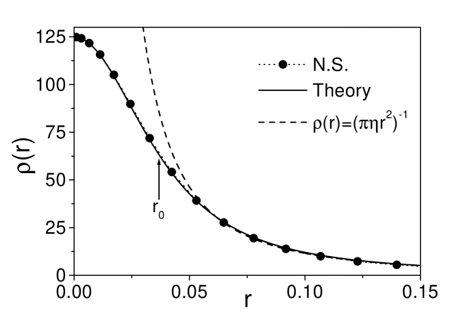
Figure 11: We plot the numerical finite-time density profile for $\eta=2.75$ (N.S.), at a time for which the central density is $\rho(0,t)\approx 124.9\approx 28.8\rho_{\infty}$. This is compared to the exact scaling profile $\rho_{0}f(r/r_{0})$ (Theory), with $f$ given by Eq. (38), and $\rho_{0}=\frac{2\pi}{3}\rho(0,t)\approx 261.6$ and $r_{0}=(\eta\rho_{0})^{-1/2}\approx 0.0373$ ($\rho(r_{0},t)/\rho(0,t)=14/27\approx 0.519$). We also plot the asymptotic density profile, $\rho_{\rm as}=(\pi\eta r^{2})^{-1}$, valid for $r_{0}\ll r\ll 1$. In this region, the correction to scaling is negligible.

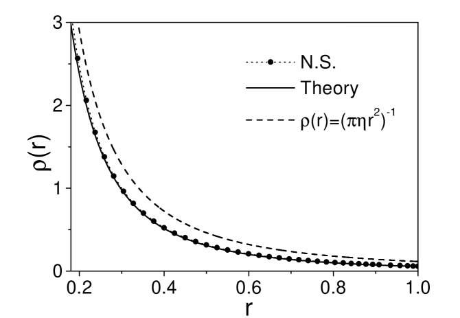
Figure 12: We plot the same numerical data (N.S.) as in Fig. 11, but in the range $5r_{0}\leq r\leq 1$. This is compared with the theoretical density profile at $t=t_{coll}$ obtained from Eqs. (48) and (57). The parameters $a\approx 5.0$ and $b\approx 5.1$ are determined by maximizing $\rho(1)$ (see text), although the full profile barely depends on $a$ and $b$, as soon as $b$ remains slightly greater than $a$, and $b\approx 4.8\sim 5.4$. In this range, the theoretical profile is in excellent agreement with the numerical one. For instance, $\rho(1)_{\rm N.S.}\approx 0.058$ and $\rho(1)_{\rm Theory}\approx 0.057$. In order to stress the quantitative agreement, we also plot the naive large $r$ asymptotics of the scaling profile $\rho_{\rm as}=(\pi\eta r^{2})^{-1}$, for which $\rho(1)_{\rm as}\approx 0.116$.

Figure 13: Time evolution of the inverse central density for $\eta=3.5$. This curve displays a scaling regime $1/\rho(0,t)=B(t_{coll}-t)$. The slope $B\simeq 2$ is close to the theoretical prediction $2\pi/3\simeq 2.1$.

In Fig. 14, we study the early development of the instability for $\eta\sim\eta_{c}$. More specifically, we start the simulations from a point on the spiral of Fig. 1 with $\eta=2.510$ and ${\cal R}=42\gtrsim 32.1$. This isothermal sphere is linearly unstable in the canonical ensemble as it is a saddle point of free energy (see Sec. 2.3) and the perturbation profile that develops for short times is shown in Fig. 14. It is in excellent agreement with the first mode of instability calculated by Chavanis [10] in the canonical ensemble. This profile does not present a “core-halo” structure, in contrast with the first mode of instability in the microcanonical situation. We have also plotted the perturbation profile for an isothermal sphere located near the second extremum of temperature ($\eta=1.842...$) at which a new mode of instability appears [10]. This second mode of instability has a core-halo structure (Fig. 15). Of course, the perturbation profile that develops is a superposition of the first two modes of instability, but we see that its structure is dominated by the contribution of the second mode.

Figure 14: First mode of instability in the canonical ensemble. The clean line is obtained by solving the eigenvalue equation (27) with $\lambda=0$ and the broken line is obtained from the numerical simulation of the SP system. The density profile does not present a “core-halo” structure.

Figure 15: Second mode of instability in the canonical ensemble.

In order to check the inequivalence of microcanonical and canonical ensembles in the region of negative specific heats, we started the simulation from an isothermal sphere with a density contrast comprised between $32.1$ and $709$. In the first experiment, the energy is kept fixed using the constraint (9). In that case, it is found that the sphere is linearly stable as it is a local entropy maximum. However, if the temperature is fixed instead of the energy, the sphere is now unstable as it is a saddle point of free energy. This clearly demonstrates in the framework of our simple dynamical model that the microcanonical and canonical ensembles are not interchangeable for self-gravitating systems. This particular circumstance can be traced back to the non-extensivity of the system due to the long-range nature of the gravitational potential. This interesting problem is discussed in the review of Padmanabhan [1] and illustrated by Chavanis [27] for specific models of self-gravitating systems with a short-range cutoff (self-gravitating fermions and hard-spheres models).

Figure 16: Basin of attraction in the canonical ensemble. The isothermal spheres located after the first turning point of the spiral are unstable in the canonical ensemble. Depending on their position on the spiral (and the initial perturbation), they can either relax towards the local maximum of free energy with same temperature ($\bullet$) or undergo a gravitational collapse ($\triangle$).

Since the stable isothermal configurations are only metastable (i.e., local maxima of a thermodynamical potential), the value of energy or temperature is not sufficient to completely determine the evolution of the system: depending on the shape of the density profile, an initial configuration with $\Lambda<\Lambda_{c}$ or $\eta<\eta_{c}$ can either reach a quiescent equilibrium state or collapse. The actual evolution of the system depends whether the initial configuration lies in the “basin of attraction” of the local entropy maximum or not. Of course, the complete characterization of this basin of attraction is an impossibly complicated task because we would have to test all possible initial configurations. We have limited our study in the canonical ensemble to the case of unstable isothermal spheres located after the first turning point of temperature. These solutions correspond to saddle points of free energy. Therefore, a small perturbation (due here to numerical roundoff error) can destabilize the system and induce a dynamical evolution. The question is whether the system evolves towards the local maximum of free energy or undergoes gravitational collapse. Since we start from a saddle point of free energy, the two evolutions are possible depending on the form of the perturbation. In addition, depending on the location of the saddle point on the spiral (its density contrast), one of these evolutions may be preferred. The results of our study are displayed in Fig. 16. The isothermal spheres that experienced a complete collapse in our numerical experiments are marked with a symbol $\triangle$ while those that converged towards an equilibrium state are marked with a symbol $\bullet$. A kind of structure seems to emerge: it appears that the isothermal spheres undergoing gravitational collapse in the canonical ensemble are concentrated near the vertical tangent. We have found a similar structure in the microcanonical ensemble with a concentration of points undergoing gravitational collapse concentrated this time near the lower horizontal tangent. However, as indicated previously, this apparent structure is relevant at best in an average sense since other initial perturbations of the same saddle point may lead to a different evolution. In any case, these results confirm that the maxima of entropy or free energy are not global maxima since they do not attract all initial conditions. While homogeneous spheres with $\Lambda<\Lambda_{c}$ and $\eta<\eta_{c}$ always seem to converge towards equilibrium, centrally concentrated systems with the same control parameters can develop a self-similar collapse leading to a finite time singularity. In fact, considering Fig. 16 again, we see that the central concentration is not the only condition for collapse since there exists highly concentrated states that also converge towards the smooth equilibrium profile with low density contrast (in that case, the evolution corresponds to an “explosion”). Therefore, the basin of attraction of the metastable equilibrium states seems to have a highly non trivial structure. The nonlinear stability of a linearly stable isothermal sphere (located this time before the first turning point of energy or temperature) is also of interest. Since it is not a global entropy maximum it can be in principle destabilized by a finite amplitude perturbation. However, this perturbation is expected to be huge so that, in practice, the stability of the isothermal spheres with low density contrast is extremely robust. This suggests that these metastable states can be very long lived [28, 29, 30] and physically relevant in an astrophysical context.

5 Conclusion

This paper has discussed the thermodynamics and the collapse of a system of self-gravitating Brownian particles in a high friction limit. This approximation considerably simplifies the problem since the evolution of the full distribution function $f({\bf r},{\bf v},t)$ is simply replaced by the evolution of its lowest moments. We showed that the Smoluchowski-Poisson system presents a rich variety of behaviors and displays interesting phase transitions between equilibrium states and collapsing states depending on the value of energy and temperature. When the two evolutions are possible, the choice depends on a complicated notion of basin of attraction. This simple model also illustrates dynamically the inequivalence of statistical ensembles for systems with long-range interactions.

An extension of our study is to consider rotating systems with conservation of angular momentum. The SP system can be generalized to include rotation [20] and is interesting to study isothermal configurations that are not spherically symmetric. When spherical symmetry is broken, it is possible that the system will fragment in several clumps and that these clumps will themselves fragment in substructures. This may yield a hierarchy of structures fitting one into each other in a self-similar way as suggested by theoretical considerations [31, 10]. It would be of interest to investigate whether the SP system can display a process of fragmentation and exhibit a fractal behavior. Numerical simulations are under way.

There exists a close analogy between the statistical mechanics of self-gravitating systems and two-dimensional vortices [32, 33, 34]. Following the pioneering work of Onsager [35], there has been some attempts to describe vortices as maximum entropy structures, with possible applications to oceanic and atmospheric situations (e.g., Jupiter’s Great Red Spot). The relaxation towards the maximum entropy state is usually described by a Smoluchowski-Poisson system which analyzes the evolution of the vorticity in terms of a diffusion and a drift. The diffusion is due to the fluctuations of the velocity field and the drift to the inhomogeneity of the vorticity field [36]. The SP system can be deduced directly from the Liouville equation by using projection operator technics [37] or from a phenomenological maximum entropy production principle [38]. It is interesting to note that, for point vortices, the Fokker-Planck equation directly has the form of a Smoluchowski equation whereas for material particles this is true only in a high friction limit. This is because, for point vortices, the phase space coincides with the configuration space while for material particles it involves the positions and the velocities of the particles.

The Smoluchowski-Poisson system also appears in the description of biological systems like bacterial populations [39]. The diffusion is due to ordinary Brownian motion and the drift models a chemically directed movement (chemotactic flux) along a concentration gradient (of smell, infection, food,…). When the attractant concentration is itself proportional to the bacterial density, this results in a coupled system morphologically similar to the one studied in the present paper. The question that naturally emerges is whether this coupling can lead to an instability for bacterial populations similar to the gravitational collapse of self-gravitating systems. This possibility will be considered in a forthcoming paper in which we consider self-similar solutions of the Smoluchowski-Poisson equation for different systems in various space dimensions [26].

6 Acknowledgments

Preliminary results of this work were presented at the conference on Multiscale Problems in Science and Technology (Dubrovnik, Sep 2000). One of us (P.H.C.) is grateful to W. Jaeger for mentioning the connection of this work with biological systems. This research was supported in part by the National Science Foundation under Grant No. PHY94-07194.

Appendix A Analytical study of the scaling equation

In this Appendix, we study analytically the scaling equation (33). To that purpose, we rewrite it in an equivalent albeit more convenient form. Let us introduce the function

(90) $$g(x)=4\pi\int_{0}^{x}f(x^{\prime})x^{{}^{\prime}2}dx^{\prime},$$

in terms of which Eq. (33) becomes

(91) $$f(x)+{x\over\alpha}f^{\prime}(x)={1\over x^{2}}{d\over dx}\{x^{2}f^{\prime}(x)+f(x)g(x)\}.$$

Multiplying both sides of equation (91) by $x^{2}$ and integrating the resulting expression between $0$ and $x$, we obtain

(92) $$g(x)=4\pi x^{2}{xf(x)-\alpha f^{\prime}(x)\over 3-\alpha+4\pi\alpha f(x)}.$$

From Eqs. (90) and (92), we can derive a nonlinear recursion relation satisfied by the coefficients $a_{n}$ of the series expansion of $f(x)$ in powers of $x^{2}$ (as $f$ is an even function). Writing

(93) $$f(x)={1\over 4\pi}\sum_{n=0}^{+\infty}(-1)^{n}a_{n}x^{2n},$$

we find

(94) $$a_{n+1}=-{2n+\alpha\over 2\alpha(n+1)(2n+3)}a_{n}+{1\over 2(n+1)}\sum_{p=0}^{n}{a_{p}a_{n-p}\over 2p+3}.$$

This recursion relation leads to the large $n$ behavior of $a_{n}$:

(95) $$a_{n}\sim 8r\biggl{(}n+{3\over 2}\biggr{)}r^{n}+o(r^{n}),$$

where $r$ is an unknown constant related to the inverse radius of convergence of the series. For $\alpha=2$, the asymptotics given by Eq. (95) with $r=1/2$ is an exact solution of the recursion relation (94), as can be checked by direct substitution. Using the identities

(96) $$P(x)={1\over 1+rx^{2}}=\sum_{n=0}^{+\infty}(-1)^{n}r^{n}x^{2n},\qquad P^{\prime}(x)=-{2rx\over(1+rx^{2})^{2}}={2\over x}\sum_{n=0}^{+\infty}(-1)^{n}nr^{n}x^{2n},$$

the series (93) can easily be resummed leading to Eq. (38).

Appendix B The case of cold systems ($T=0$)

For $T=0$, the core radius is not given by the King radius (29) which is zero by definition. We still assume however that $\rho_{0}\overline{r}_{0}^{\alpha}\sim 1$, where $\alpha$ is unknown a priori. The equation for the invariant profile is then given by

(97) $$f(x)+{x\over\alpha}f^{\prime}(x)={1\over x^{2}}{d\over dx}(f(x)g(x)),$$

where $g(x)$ is defined by Eq. (90). Multiplying Eq. (97) by $4\pi x^{2}$ and integrating from $0$ to $x$ we obtain

(98) $$g(x)={4\pi x^{3}f(x)\over 3-\alpha+4\pi\alpha f(x)}.$$

Using the relation $f(x)=g^{\prime}(x)/4\pi x^{2}$, the foregoing equation can be rewritten

(99) $$(\alpha-3)g(x)+xg^{\prime}(x)=\alpha{1\over x^{2}}g^{\prime}(x)g(x).$$

Introducing the change of variables $u=x^{3}$, we get

(100) $$3{dg\over du}={(3-\alpha)g\over u-\alpha g}.$$

A separation of the variables can be effected by the transformation $g=uh$, yielding

(101) $${1-\alpha h\over h(3h-1)}dh={\alpha\over 3}{du\over u}.$$

This equation is readily integrated leading to the implicit equation

(102) $$g(x)=\lambda\biggl{(}{x^{3}\over 3}-g(x)\biggr{)}^{1-\alpha/3},$$

where $\lambda$ is an integration constant. As $g(x)$ is an odd analytical function, Eq. (102) first implies that $g(x)\sim{x^{3}\over 3}$, so that $f(0)={1\over 4\pi}$. Combining with Eq. (32), this yields $\rho(0,t)={\xi\over 4\pi G}(t_{coll}-t)^{-1}$. Then, inserting $g(x)-{x^{3}\over 3}\sim x^{5}$ in Eq. (102), we find that $x^{3}\sim x^{5(1-\alpha/3)}$, leading to $\alpha=6/5$. Note finally that the scaling profile defined by the implicit equation (102) can be written in the parametric form

(103) $$f(x)={1\over 4\pi}{1\over 1+s},\qquad g(x)={1\over 3}s^{3/2},\qquad x=s^{1/2}\biggl{(}1+{3\over 5}s\biggr{)}^{1/3},$$

where the constant $\lambda$ has been incorporated in the expression of the core radius $\overline{r}_{0}$.

In fact, for $T=0$, Eq. (6) can be solved analytically. Since the diffusion term vanishes, this equation describes a deterministic motion where the particles have a velocity ${\bf u}=-{1\over\xi}\nabla\Phi$ directly proportional to the gravitational force (see Sec. 2.1). This deterministic problem can be solved exactly by adapting the procedure followed by Penston [4] in his investigation of the collapse of cold self-gravitating gaseous spheres. Let us consider a particle located at $r(0)=a$ at time $t=0$. We denote by $\overline{\rho}(a)$ the average density inside the sphere of radius $a$. The total mass inside radius $a$ can therefore be expressed as $M_{a}={4\pi\over 3}\overline{\rho}(a)a^{3}$. At time $t$, this mass is now contained in the sphere of radius $r=r(t)$, where $r(t)$ is the position of the particle initially at $r=a$. Using the Gauss theorem, the motion of the particle is described by the first order differential equation

(104) $${dr\over dt}=-{1\over\xi}{GM_{a}\over r^{2}}.$$

This equation can be integrated explicitly to give

(105) $$r=a\biggl{(}1-{4\pi G\over\xi}\overline{\rho}(a)t\biggr{)}^{1/3}.$$

Let us first discuss the case where the system is initially homogeneous with density $\overline{\rho}(a)=\overline{\rho}_{0}$. In that case, all the particles (whatever their initial position) arrive at $r=0$ at a time $t_{coll}={\xi/4\pi G\overline{\rho}_{0}}$ defined as the collapse time for $T=0$. This expression represents a lower bound (reached for $\eta\rightarrow+\infty$) on the value of the collapse time $t_{coll}(\eta)$ studied in Sec. 3.4. During the evolution, the sphere remains homogeneous with radius, density and free energy evolving as

(106) $$R(t)=R(1-t/t_{coll})^{1/3},\quad\rho(t)=\overline{\rho}_{0}(1-t/t_{coll})^{-1},\quad J(t)={3\beta GM^{2}\over 5R}(1-t/t_{coll})^{-1/3}.$$

Note that the free energy diverges at $t=t_{coll}$, unlike in Sec. 3.2. These results can also be obtained directly from Eq. (6) which reduces, for a uniform density, to

(107) $${d\rho\over dt}=\nabla\biggl{(}{1\over\xi}\rho\nabla\Phi\biggr{)}={1\over\xi}\rho\Delta\Phi={4\pi G\over\xi}\rho^{2},$$

where we have used the Poisson equation (5) to get the last equality.

We now suppose that, initially, $\overline{\rho}(a)$ has a smooth maximum at the center so that

(108) $$\overline{\rho}(a)=\overline{\rho}_{0}\biggl{(}1-{a^{2}\over A^{2}}\biggr{)},$$

for sufficiently small $a$, where $A$ is a constant. In that case, Eq. (105) giving the position at time $t$ of the particle located at $r=a$ at $t=0$ becomes

(109) $$r=a\biggl{[}1-\biggl{(}1-{a^{2}\over A^{2}}\biggr{)}{t\over t_{coll}}\biggr{]}^{1/3}.$$

At $t=t_{coll}$, the time at which the central density becomes infinite, it reduces to $r={a^{5/3}/A^{2/3}}$. It is now straightforward to obtain the full density profile at $t=t_{coll}$. Since the mass contained between $a$ and $a+da$ at $t=0$ arrives between $r$ and $r+dr$ at time $t$, we have in full generality

(110) $$\overline{\rho}(a)4\pi a^{2}da=\rho(r,t)4\pi r^{2}dr,$$

or, for sufficiently small $a$,

(111) $$\rho(r,t)=\overline{\rho}(a){a^{2}\over r^{2}}{da\over dr}\simeq\overline{\rho}_{0}{a^{2}\over r^{2}}{da\over dr}.$$

At $t=t_{coll}$, we get

(112) $$\rho(r,t_{coll})={3\over 5}\overline{\rho}_{0}A^{6/5}r^{-6/5}.$$

We have therefore recovered that, for $T=0$, the density profile decreases algebraically with an exponent $\alpha=6/5$. We now extend this analysis to a time $\tau=t_{coll}-t$ just before the singularity arises. Considering the limit $a\rightarrow 0$ and $\tau\rightarrow 0$, Eq. (109) can be expanded to lowest order as

(113) $$r=a\biggl{(}{\tau\over t_{coll}}+{a^{2}\over A^{2}}\biggr{)}^{1/3}.$$

Then, Eq. (111) leads, after some reductions, to the density profile

(114) $$\rho(r,t)={\overline{\rho}_{0}\over{\tau\over t_{coll}}+{5a^{2}\over 3A^{2}}}.$$

The central density corresponds to $r=0$, i.e. $a=0$. According to Eq. (114) it evolves with time as

(115) $$\rho(0,t)={\overline{\rho}_{0}t_{coll}\over\tau}={\xi\over 4\pi G}(t_{coll}-t)^{-1}.$$

Therefore, if we define

(116) $$s={5a^{2}t_{coll}\over 3A^{2}\tau},\qquad\overline{r}_{0}=\biggl{(}{3A^{2}\over 5}\biggr{)}^{1/2}\biggl{(}{\tau\over t_{coll}}\biggr{)}^{5/6}.$$

we can express the density profile in the parametric form

(117) $${\rho(r,t)\over\rho(0,t)}={1\over 1+s},\qquad{r\over\overline{r}_{0}(t)}=s^{1/2}\biggl{(}1+{3\over 5}s\biggr{)}^{1/3},$$

which is equivalent to Eq. (103). According to Eq. (115) and (116), we have the scaling laws $\overline{r}_{0}\sim(t_{coll}-t)^{5/6}$, $\rho(0)\overline{r}_{0}^{6/5}\sim 1$ just before the singularity occurs. Setting $F=\rho/\rho(0)$ and $x=r/\overline{r}_{0}$, we easily check that $F(x)=1-x^{2}+...$ for $x\rightarrow 0$ and $F(x)\sim({3/5})^{2/5}x^{-6/5}$ for $x\rightarrow+\infty$. This solves the problem for $T=0$. Now, if the temperature $T$ is very small but non-zero, we expect the present scaling to hold provided that $\overline{r}_{0}\gg r_{0}(t)$, where $r_{0}$ is defined in section 3. This leads to a cross-over core density $\rho_{0}^{*}$ above which the $T\neq 0$ scaling of section 3.2 will prevail. The density $\rho_{0}^{*}$ can be estimated by equating $r_{0}=(T/G\rho_{0})^{1/2}$ to $\overline{r}_{0}\sim\rho_{0}^{-5/6}$. The $T\neq 0$ scaling then prevails when the density becomes high enough, $\rho_{0}^{*}\sim({T/G})^{-3/2}$.

Appendix C Connection between dynamical and thermodynamical stability

Let $\rho$ be a stationary solution of Eq. (6) and $\delta\rho$ a small perturbation around this solution. The first and second variations of temperature respecting the energy constraint (9) can be expressed as

(118) $${3\over 2}M\delta T+\int\delta\rho\Phi\,d^{3}{\bf r}=0,$$

(119) $${3\over 2}M\delta^{2}T+{1\over 2}\int\delta\rho\delta\Phi\,d^{3}{\bf r}=0.$$

The critical point $\rho$ is a local entropy maximum provided that the second variations of entropy

(120) $$\delta^{2}S=-{3M\over 4}{(\delta T)^{2}\over T^{2}}+{3M\over 2}{\delta^{2}T\over T}-{1\over 2}\int{(\delta\rho)^{2}\over\rho}\,d^{3}{\bf r}$$

are negative for any variations that conserve mass to first order. Let us now linearize Eq. (6) around equilibrium and write the time dependence of the perturbation in the form $\delta\rho\sim e^{\lambda t}$. We get

(121) $$\lambda\delta\rho=\nabla\biggl{[}{1\over\xi}(\delta T\nabla\rho+T\nabla\delta\rho+\delta\rho\nabla\Phi+\rho\nabla\delta\Phi)\biggr{]}.$$

Multiplying both sides of Eq. (121) by $\delta\rho/\rho$, integrating by parts and using the equilibrium condition $T\nabla\rho+\rho\nabla\Phi=0$, we obtain

(122) $$\lambda\int{(\delta\rho)^{2}\over\rho}\,d^{3}{\bf r}=-\int{1\over T\rho\xi}(T\nabla\delta\rho+\delta\rho\nabla\Phi)(\delta T\nabla\rho+T\nabla\delta\rho+\delta\rho\nabla\Phi+\rho\nabla\delta\Phi)\,d^{3}{\bf r}.$$

We now remark that the second order variations of the rate of entropy production (11) are given by

(123) $$\delta^{2}\dot{S}=\int{1\over\rho T\xi}(\delta T\nabla\rho+T\nabla\delta\rho+\delta\rho\nabla\Phi+\rho\nabla\delta\Phi)^{2}\,d^{3}{\bf r}.$$

We can therefore rewrite Eq. (122) in the form

$$\lambda\int{(\delta\rho)^{2}\over\rho}\,d^{3}{\bf r}=-\delta^{2}\dot{S}+\int{1\over T\rho\xi}(\delta T\nabla\rho+\rho\nabla\delta\Phi)$$

(124) $$\times(\delta T\nabla\rho+T\nabla\delta\rho+\delta\rho\nabla\Phi+\rho\nabla\delta\Phi)\,d^{3}{\bf r}.$$

Using the equilibrium condition, the last term in Eq. (124) is clearly the same as

(125) $$-\int{1\over\xi}(\delta T\nabla\rho+T\nabla\delta\rho+\delta\rho\nabla\Phi+\rho\nabla\delta\Phi)\biggl{(}{\delta T\over T^{2}}\nabla\Phi-{1\over T}\nabla\delta\Phi\biggr{)}\,d^{3}{\bf r}.$$

Taking the time derivative of Eq. (9) and using Eq. (6) we have at each time

(126) $$\dot{E}={3\over 2}M\dot{T}-\int{1\over\xi}(T\nabla\rho+\rho\nabla\Phi)\nabla\Phi\,d^{3}{\bf r}=0.$$

The energy constraint (126) must be satisfied to first and second order. This yields:

(127) $$\int{1\over\xi}(\delta T\nabla\rho+T\nabla\delta\rho+\delta\rho\nabla\Phi+\rho\nabla\delta\Phi)\nabla\Phi\,d^{3}{\bf r}={3\over 2}M\delta\dot{T}={3\over 2}M\lambda\delta{T},$$

(128) $$\int{1\over\xi}(\delta T\nabla\rho+T\nabla\delta\rho+\delta\rho\nabla\Phi+\rho\nabla\delta\Phi)\nabla\delta\Phi\,d^{3}{\bf r}={3\over 2}M\delta^{2}\dot{T}={3}M\lambda\delta^{2}{T},$$

where we have used Eqs. (118)-(119) to obtain the last equalities. Substituting these relations in Eq. (124), we get

(129) $$\lambda\biggl{\{}\int{(\delta\rho)^{2}\over\rho}\,d^{3}{\bf r}+{3M\over 2}{(\delta T)^{2}\over T^{2}}-3M{\delta^{2}T\over T}\biggr{\}}=-\delta^{2}\dot{S}.$$

Comparing with Eq. (120), we finally obtain

(130) $$\delta^{2}\dot{S}=2\lambda\delta^{2}S.$$

Since $\delta^{2}\dot{S}\geq 0$, see Eq. (123), the sign of $\lambda$ is the same as that of $\delta^{2}S$. If $\rho$ is a local entropy maximum, then $\delta^{2}S$ and consequently $\lambda$ are negative for any perturbation: the solution is linearly stable. Otherwise, we can find a perturbation for which $\delta^{2}S$, and consequently $\lambda$, are positive: the solution is linearly unstable. We can easily extend the relation (130) to the canonical ensemble with $J$ instead of $S$. We have found the same relation for other types of kinetic equations (Chavanis, in preparation), so its validity seems to be of a very wide scope.

References

- [1] T. Padmanabhan, Phys. Rep. 188, 285 (1990).
- [2] V.A. Antonov, Vest. Leningr. Gos. Univ. 7, 135 (1962).
- [3] D. Lynden-Bell and R. Wood, Mon. Not. R. astr. Soc. 138, 495 (1968).
- [4] M.V. Penston, Mon. Not. R. astr. Soc. 144, 425 (1969).
- [5] R.B. Larson, Mon. Not. R. astr. Soc. 147, 323 (1970).
- [6] H. Cohn, Astrophys. J. 242, 765 (1980).
- [7] D. Lynden-Bell and P.P. Eggleton, Mon. Not. R. astr. Soc. 191, 483 (1980).
- [8] C. Lancellotti and M. Kiessling, Astrophys. J. 549, L93 (2001).
- [9] T. Padmanabhan, Astrophys. J. Supp. 71, 651 (1989).
- [10] P.H. Chavanis, Astron. Astrophys. 381, 340 (2002).
- [11] H. Risken, The Fokker-Planck equation (Springer, 1989).
- [12] S. Chandrasekhar, Rev. Mod. Phys. 21, 383 (1949).
- [13] D. Lynden-Bell, Mon. Not. R. astr. Soc. 136, 101 (1967).
- [14] P.H. Chavanis, Mon. Not. R. astr. Soc. 300, 981 (1998).
- [15] P.H. Chavanis, Astron. Astrophys. 356, 1089 (2000).
- [16] R.F. Streater, J. Stat. Phys. 88, 447 (1997).
- [17] R.F. Streater, Statistical Dynamics (Imperial College Press, 1995)
- [18] P. Biler, A. Krzywicki and T. Nadzieja, Rep. Math. Phys. 42, 359 (1998).
- [19] C. Rosier, C. R. Acad. Sci. Paris, Série I Math. 332, 903 (2001).
- [20] P.H. Chavanis, J. Sommeria and R. Robert, Astrophys. J. 471, 385 (1996).
- [21] P.H. Chavanis, Statistical mechanics of violent relaxation in stellar systems in Proceedings of the Conference on Multiscale Problems in Science and Technology, edited by N. Antonic, C.J. van Duijn, W. Jäger, and A. Rikelic (Springer, Berlin, 2002).
- [22] J. Binney and S. Tremaine, Galactic Dynamics (Princeton Series in Astrophysics, 1987).
- [23] S. Chandrasekhar, An Introduction to the Theory of Stellar Structure (Dover, 1942).
- [24] J. Katz, Mon. Not. R. astr. Soc. 183, 765 (1978).
- [25] M. Kiessling, J. Stat. mech. 55, 203 (1989).
- [26] C. Sire and P.H. Chavanis, e-print cond-mat/0204303.
- [27] P.H. Chavanis, Phys. Rev. E 65, 056123 (2002).
- [28] H.A. Posch and W. Thirring, Physica A 194, 482 (1993).
- [29] V.P. Youngkins and B.N. Miller, Phys. Rev. E 62, 4582 (2000).
- [30] P.H. Chavanis and I. Ispolatov, e-print cond-mat/0205204.
- [31] B. Semelin, H.J. de Vega, N. Sanchez and F. Combes, Phys. Rev. D 59, 125021 (1999).
- [32] P.H. Chavanis, PhD. thesis, Ecole Normale Supérieure de Lyon, 1996.
- [33] P.H. Chavanis, Ann. (N.Y.) Acad. Sci. 867, 120 (1998).
- [34] P.H. Chavanis, On the analogy between two-dimensional vortices and stellar systems, in Proceedings of the IUTAM Symposium on Geometry and Statistics of Turbulence, Hayama (Kluwer Academic, Dordrecht, 2000).
- [35] L. Onsager, Nuovo Cimento Suppl. 6, 279 (1949).
- [36] P.H. Chavanis, Phys. Rev. E 58, R1199 (1998).
- [37] P.H. Chavanis, Phys. Rev. E 64, 026309 (2001).
- [38] R. Robert and J. Sommeria, Phys. Rev. Lett. 69, 2776 (1992).
- [39] J.D. Murray, Mathematical Biology (Springer, 1991).