[

Anomalous Lévy decoherence

Abstract

We investigate the decoherence of a small quantum system weakly coupled to a complex, chaotic environment when the dynamics is not Gaussian but Lévy anomalous. By studying the time dependence of the linear entropy and the damping of the interference of two Gaussian wave packets in the Wigner representation, we show that the decoherence time for a quantum Lévy stable process is always smaller than for Gaussian diffusion.

] First a subject of mathematical investigation [1, 2], Lévy stable processes have nowadays fully entered the realm of physics [3, 4]. It is well known that usual Brownian motion is a Gaussian stochastic process [5]. This is a consequence of the Gaussian law of large numbers, or central–limit theorem. In the 1930s, the central–limit theorem has been extended by Lévy and others to random variables with infinite second moment. More precisely, the probability distribution of these random variables has the form,

$${\cal L}^{\scriptscriptstyle{C}}_{\alpha}(x)=\frac{1}{2\pi}\int_{-\infty}^{\infty}e^{ikx-C|k|^{\alpha}}dk\ ,\hskip 14.22636pt0<\alpha\leq 2\ .$$ (1)

A (symmetric) Lévy stable distribution as given by (1) can be regarded as an extension of the Gaussian distribution to which it reduces when $\alpha\!=\!2$. It should be stressed, however, that the Gaussian distribution is the only stable law having a finite variance. A Lévy process may then be defined as a non–Gaussian generalization of Brownian motion obeying Lévy stable statistics. The hallmark of this form of anomalous diffusion is the presence of long jumps (the so–called “Lévy flights”) which are due to the asymptotic power–law tail of a stable distribution, ${\cal L}^{\scriptscriptstyle{C}}_{\alpha}(x)\sim 1/|x|^{\alpha+1}$. As a consequence, the mean–square displacement and the mean kinetic energy of a Lévy particle are divergent [6]. Lévy dynamics often results from the interaction with a complex, non-homogeneous environment. Examples are porous or disordered media [7] or chaotic heat baths [8].

The first experimental observation of a Lévy stable process has been reported ten years ago in micelle systems [9]. Since then, Lévy–like diffusion has for instance been seen in two–dimensional rotating flows [10], in porous glasses [11] and, more recently, in ion lattices [12] and in subrecoil laser cooling [13]. The ion lattice experiment is of particular interest since it reports a direct measurement of the divergence of the mean kinetic energy of the particle. Moreover, it is worthwhile to notice that experiments have now started to study anomalous Lévy dynamics of microscopic systems (atoms, ions) where quantum effects are likely to play a role. This motivated us to examine the decoherence of quantum Lévy stable motion.

Decoherence manifests itself in the dynamical destruction of quantum interferences as a result of the interaction with the environment [14]. This progressive transition from quantum to classical has been experimentally observed in high Q microwave cavities [15]. Theoretically, decoherence has been intensively investigated in the case of normal (Gaussian) diffusion [16, 17, 18] but not so far for anomalous Lévy diffusion.

A simple way to evaluate the decoherence time $\tau^{\alpha}_{D}$ is to compute the linear entropy $S_{\alpha}(t)=1-\mbox{tr}\rho^{2}(t)$, which gives a measure of the purity of the system [19, 20]: The linear entropy is equal to zero for a pure state and increases to one when the state of the system evolves to a mixture. Here $\rho(t)$ is the reduced density operator of the system. Alternatively, one can consider the superposition of two Gaussian wave packets in the Wigner representation and look at the damping of the interference fringes [21]. In the following we study the time dependence of both the linear entropy and of the interference term of the Wigner function. We put a special emphasis on the value $\alpha=1$ where analytical results can be obtained. What we find is that Lévy decoherence is always faster than Gaussian decoherence for any value of the stability index $\alpha$.

Starting point of our analysis is a master equation for a system coupled to a chaotic environment derived by Kusnezov et al. from a microscopic random–matrix model [8]. In this approach the coupling to the non–homogeneous background is characterized by a spreading width $\Gamma^{\downarrow}$ and a spatial correlation function $G(x/x_{0})$ with an environment characteristic correlation length $x_{0}$ (see Ref. [8] for details). In the limit of high (actually infinite) temperature, the quantum master equation for a free particle of mass $M$ is given by

$$\frac{\partial}{\partial t}\rho(x,y,t) = -\frac{i\hbar}{2M}\Big{[}\frac{\partial^{2}}{\partial x^{2}}-\frac{\partial^{2}}{\partial y^{2}}\Big{]}\rho(x,y,t)$$ (2)

$$- \frac{\Gamma^{\downarrow}}{\hbar}\Big{[}G\Big{(}\frac{x-y}{x_{0}}\Big{)}-1\Big{]}\rho(x,y,t)\ .$$ (3)

When the environment correlation length $x_{0}$ is much larger than the separation $\Delta x=|x-y|$, the correlator in Eq. (2) can be expanded as[22]

$$G\left(\frac{\Delta x}{x_{0}}\right)=1-\left|\frac{\Delta x}{x_{0}}\right|^{\alpha}\ .$$ (4)

The case $\alpha\!=\!2$ corresponds to Gaussian diffusion, while for a faster spatial decorrelation, $0<\!\alpha\!<2$, the diffusion is Lévy anomalous [8, 23]. The (generalized) diffusion coefficient is further defined as $D_{\alpha}=\Gamma^{\downarrow}/(\hbar x_{0}^{\alpha})$. It is also worthwhile to emphasize that it is the last term in the master equation (2), which results from the accumulation of phase fluctuations of the environment, which is mainly responsible for the decoherence effect [14]. We already know that the alteration of this noise term when passing from Gauss to Lévy statistics has a dramatic effect on the diffusion properties of the system, it is thus of high interest to examine the effect of the modification of this term on decoherence.

We begin by solving the master equation (2) for $\rho(t)$. For this purpose it is convenient to use the $(k,\Delta)$ representation of the density matrix [24],

$$\rho(k,\Delta,t)=\int_{-\infty}^{\infty}dq\,e^{ikq}\,\rho(q+\frac{\Delta}{2},q-\frac{\Delta}{2},t)\ ,$$ (5)

instead of the coordinate representation $\rho(x,y,t)$. Here, we have introduced the center of mass and relative coordinates, $q=(x+y)/2$ and $\Delta=x-y$. In this representation, the master equation reads

$$\frac{\partial}{\partial t}\rho(k,\Delta,t)=\Big{\{}\frac{k}{M}\frac{\partial}{\partial\Delta}-D_{\alpha}|\Delta|^{\alpha}\Big{\}}\rho(k,\Delta,t)\ .$$ (6)

This first order partial differential equation can easily be solved, for instance by the method of characteristics . We find

$$\rho(k,\Delta,t) = \rho(k,\Delta+\frac{kt}{M},0)\,\exp\left[-\frac{MD_{\alpha}}{(1+\alpha)k}\left(\Delta+\frac{kt}{M}\right)\right.$$ (8)

$$\times\left.\left|\Delta+\frac{kt}{M}\right|^{\alpha}\right]\exp\left[\frac{MD_{\alpha}}{(1+\alpha)k}\,\Delta|\Delta|^{\alpha}\right]\ ,$$

where $\rho(k,\Delta,0)$ is the reduced density operator at $t=0$. For an initial Gaussian pure state, $\rho(x,y,0)\!=\!\varphi(x)\varphi^{*}(y)$ with $\varphi(x)=\exp[-x^{2}/4b^{2}]/(2\pi b^{2})^{1/4}$, it has the form

$$\rho(k,\Delta,0)=\exp\Big{[}-\frac{k^{2}b^{2}}{2}-\frac{\Delta^{2}}{8b^{2}}\Big{]}\ .$$ (9)

It is further interesting to consider the probability distributions for position and momentum that correspond to the solution (8). In the limit of long times, we have

$$\rho(x,x,t) = \int_{-\infty}^{\infty}dk\,e^{-ikx}\rho(k,\Delta\!=\!0,t)\simeq{\cal L}_{\alpha}^{u(t)}(x)\ ,$$ (10)

$$\rho(p,p,t) = \int_{-\infty}^{\infty}d\Delta\,e^{-ip\Delta}\rho(k\!=\!0,\Delta,t)\simeq{\cal L}_{\alpha}^{v(t)}(p)\ ,$$ (11)

with $u(t)=D_{\alpha}t^{1+\alpha}/(1+\alpha)M^{\alpha}$ and $v(t)=D_{\alpha}t$. The result (10), which holds for $1\!<\!\alpha\!<\!2$, has already been obtained in Ref. [8]. Notice that both the position and the momentum distributions of the system asymptotically approach a Lévy stable law (in the short time limit they are given by Gaussians). In particular, this means that for $\alpha\!=\!1$, $\rho(p,p,t)$ has the form of a Lorentzian. It is worth mentioning that a recent experiment confirmed that the momentum distribution of atoms cooled by selective coherent population trapping is very close to a Lorentzian distribution [25].

Linear entropy. Let us now calculate the linear entropy $S_{\alpha}(t)$ of the system. We use the expression (8) for $\rho(k,\Delta,t)$ together with the initial condition (9). For short times, we then obtain

$$S_{\alpha}(t) \simeq 1-\frac{1}{\sqrt{4\pi b^{2}}}\int d\Delta\,\exp\left[-\frac{\Delta^{2}}{4b^{2}}\right]\left(1-2D_{\alpha}|\Delta|^{\alpha}t\right)$$ (12)

$$= \frac{2^{\alpha+1}}{\sqrt{\pi}}\Gamma\left(\frac{1+\alpha}{2}\right)\frac{\Gamma^{\downarrow}}{\hbar}\left(\frac{b}{x_{0}}\right)^{\alpha}t\ .$$ (13)

Consequently, the system gets entangled with the environment within a decoherence time of the order of $\tau^{\alpha}_{D}\sim[(\Gamma^{\downarrow}/\hbar)(b/x_{0})^{\alpha}]^{-1}$, where $b$ is the width of the initial wave packet.

In order to obtain more tractable expressions, we will work in the following in the limit $\hbar\rightarrow 0$, where $D_{\alpha}\langle(\Delta x)^{\alpha}\rangle$ is large [18]. In this “semiclassical” limit, the time evolution of the density operator is dominated by the last term in Eq. (2). It is then straighforward to write down an approximate solution of the master equation in the form,

$$\rho(x,y,t)=\rho(x,y,0)\,\exp\left[-\frac{\Gamma^{\downarrow}}{\hbar}\left|\frac{x-y}{x_{0}}\right|^{\alpha}t\right]\ .$$ (14)

We observe that the off–diagonal matrix elements decay exponentially on a time scale $\tau^{\alpha}_{D}=[(\Gamma^{\downarrow}/\hbar)(\Delta x/x_{0})^{\alpha}]^{-1}$. Note that this expression of the decoherence time is in agreement with the previous result obtained from the short time behavior of the linear entropy. Let us briefly discuss the validity of this approximation. To this end, it is instructive to write the approximate solution (14) of the master equation in the $(k,\Delta)$ representation which yields

$$\rho(k,\Delta,t)=\rho(k,\Delta,0)\exp[-D_{\alpha}|\Delta|^{\alpha}t]\ .$$ (15)

This expression is easily seen to be a short time approximation of the exact solution (8) [see also Fig. (1)].

Superposition of wave packets. We now turn to the study of the effect of decoherence on the interference of two Gaussian wave packets in the Wigner representation. The Wigner transform of the density matrix is defined as

$$W(q,p,t)= \frac{1}{2\pi\hbar}\int_{-\infty}^{\infty}d\Delta\exp\Big{[}-\frac{ip\Delta}{\hbar}\Big{]}$$ (17)

$$\times\rho\Big{(}q+\frac{\Delta}{2},q-\frac{\Delta}{2},t\Big{)}\ .$$

We mention that the (pseudo-) phase space distribution $W(q,p,t)$ is also related to the $(k,\Delta)$ representation by a (double) Fourier transform [16]. Applying the Wigner transform to the master equation (2) (retaining again only the last term) we arrive at a fractional diffusion equation in momentum,

$$\frac{\partial}{\partial t}W(q,p,t)=D_{\alpha}\,\frac{\partial^{\alpha}}{\partial|p|^{\alpha}}W(q,p,t)\ .$$ (18)

Here the Riesz fractional derivative is defined through its Fourier transform as [26, 27],

$$-\frac{\partial^{\alpha}}{\partial|p|^{\alpha}}=\frac{1}{2\pi}\int_{-\infty}^{\infty}dz\,\exp[-ipz]\,|z|^{\alpha}\ .$$ (19)

The solution of the fractional equation (18) can for instance be found in [6]. Next we consider an initial state of our system that consists of the linear superposition of two Gaussian wave packets separated by a distance $2a$: $\psi(x)=c_{1}\exp[-(x-a)^{2}/4b^{2}]+c_{2}\exp[-(x+a)^{2}/4b^{2}]$. The Wigner function corresponding to this initial state can be written as a sum of two classical contributions plus a quantum (interference) term: $W=W_{1}+W_{2}+W_{int}$. For the value $\alpha\!=\!1$, analytical evaluation of the Wigner function $W(q,p,t)$ is possible. This leads to

$$W_{1,2}(q,p,t) = |c_{1,2}|^{2}\exp\left[-\frac{(q\pm a)^{2}}{2b^{2}}\right]f(0)\ ,$$ (20)

$$W_{int}(q,p,t) = \exp\left[\frac{a^{2}-q^{2}}{2b^{2}}\right]$$ (22)

$$\times\{c_{1}^{*}c_{2}f(a)+c_{1}c_{2}^{*}f(-a)\}\ .$$

The function $f(a)$ is given by the expression

$$f(a) = \sqrt{\frac{b^{2}}{2\pi}}\left\{\exp\left[\left(D_{\alpha}t-\left(\frac{a}{2b}-ip\right)\right)^{2}2b^{2}\right]\right.$$ (24)

$$\left.\times\left[1-\mbox{Erf}\left(\left(D_{\alpha}t-\left(\frac{a}{2b}-ip\right)\right)\sqrt{2}b\right)\right]\right.$$

$$+ \left.\exp\left[\left(D_{\alpha}t+\left(\frac{a}{2b}-ip\right)\right)^{2}2b^{2}\right]\right.$$ (26)

$$\left.\times\left[1-\mbox{Erf}\left(\left(D_{\alpha}t+\left(\frac{a}{2b}-ip\right)\right)\sqrt{2}b\right)\right]\right\}\ ,$$

$\mbox{Erf}(x)=2/\sqrt{\pi}\int_{0}^{x}\exp[-t^{2}]dx$ being the Error function. Moreover, in the limit where the two wave packets are well separated ($a\gg b$), the time dependence of the interference term can be simplified to become

$$W_{int}(q,0,t)\sim\sqrt{\frac{b^{2}}{2\pi}}\exp\left[\frac{a^{2}}{2b^{2}}-2aD_{1}t\right]\ .$$ (27)

Hence the interference between the two superposed Gaussian wave packets is exponentially destroyed by decoherence on a time $\tau^{1}_{D}=[(\Gamma^{\downarrow}/\hbar)2a/x_{0}]^{-1}$, where $2a$ is the distance between the two wave packets.

Discussion. Let us now discuss the results that we have obtained so far. We have found that for a quantum Lévy process with exponent $\alpha$, the suppression of coherence over a distance $\Delta x$ takes place exponentially on a time scale $\tau^{\alpha}_{D}\sim[(\Gamma^{\downarrow}/\hbar)(\Delta x/x_{0})^{\alpha}]^{-1}$, $\Delta x$ being either the width of the single wave packet in the computation of the linear entropy or the separation of the two packets in the evaluation of the Wigner function. The decoherence time $\tau^{\alpha}_{D}$ is hence inversely proportional to the spreading width $\Gamma^{\downarrow}$ and also inversely proportional to the $\alpha$th power of the ratio of the distance $\Delta x$ over the environment correlation length $x_{0}$. When compared to the Gaussian case $\alpha=2$, we find that $\tau^{\alpha}_{D}/\tau^{2}_{D}\sim(\Delta x/x_{0})^{2-\alpha}$, independent of the factor $\Gamma^{\downarrow}/\hbar$.

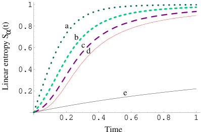
FIG. 1.: Linear entropy $S_{\alpha}(t)$ as a function of time for different values of the stability index $\alpha$: The curves $(a)$ to $(d)$ are obtained with the exact solution (8) of the master equation for increasing values of $\alpha$, $\alpha=0.5,1,1.5,2$. The curve $(e)$ corresponds to the approximate solution (15) in the case $\alpha=2$.

In the present analysis the environment correlation length $x_{0}$ is much larger than any typical system separation $\Delta x$, so that we have $\Delta x/x_{0}\ll 1$. Since for Lévy stable motion $\alpha<2$, we are therefore lead to the conclusion that Lévy decoherence is always (for any exponent $\alpha$) faster than Gaussian decoherence (or in other words its decoherence time is always smaller). The dependence of the decoherence time on the value of the stability index is shown in Fig. (1), where the linear entropy $S_{\alpha}(t)$ is plotted as a function of time for different values of the parameter $\alpha$. We see that the smaller the value of $\alpha$, the faster the decoherence for a Lévy process. For instance, for a ratio $\Delta x/x_{0}=10^{-3}$, Lévy decoherence is three orders of magnitude faster than Gaussian decoherence when $\alpha=1$. Lévy anomalous diffusion hence appears, in this sense, to be “more classical” than its Gaussian counterpart.

This result can be interpreted as follows. In the Langevin picture of Brownian motion, the coupling to the environment manifests itself in the addition of two forces to Newton’s equation: first, a friction force which dissipates energy away from the system and, second, a fluctuating stochastic force which randomly injects energy back into the system. For Lévy stable motion, the variance of this stochastic force is divergent which means that the environment randomly supplies an infinite amount of energy to the system (this is, by the way, the physical origin of the Lévy flights) [28]. Thus, in this case, the coupling to the surroundings has a much stronger influence on the evolution of the system and, in turn, decoherence, like diffusion, is greatly enhanced. Note, however, that in contrast to diffusion, Lévy decoherence does not involve divergent quantities.

In summary, we have investigated the decoherence properties of a small quantum system weakly coupled to a chaotic background when its dynamics exhibits Lévy type anomalous behavior. We have determined the decoherence time, first, by computing the linear entropy of the system and, then, by examining the decay of interference fringes of two superposed Gaussian wave packets in the Wigner representation. In comparison to the Gaussian case, we have found that Lévy decoherence is always faster. More precisely, the deviation of the decoherence time from its Gaussian value is larger the smaller the value of the characteristic exponent $\alpha$.

This work was supported by the RTD network Nanoscale Dynamics, Coherence and Computation. We thank D. Kusnezov and C. Lewenkopf for discussion.

REFERENCES

- [1] P. Lévy, Théorie de l’Addition des Variables Aléatoires, (Gauthiers–Villars, Paris, 1937).
- [2] J.L. Doob, Ann. Math. 43, 351 (1942).
- [3] Lévy Flights and Related Topics in Physics, edited by M.F. Shlesinger, G.M. Zaslavsky, and U. Frisch, (Springer, Berlin, 1994).
- [4] Anomalous Diffusion. From Basics to Applications, edited by A. Pȩkalski and K. Sznajd–Weron, (Springer, Berlin, 1998).
- [5] H. Risken, The Fokker–Planck Equation (Springer, Berlin, 1989).
- [6] S. Jespersen, R. Metzler, and H.C. Fogedby, Phys. Rev. E 59, 2736 (1999).
- [7] J.-P. Bouchaud and A. Georges, Phys. Rep. 195, 127 (1990).
- [8] D. Kusnezov, A. Bulgac, and G. Do Dang, Phys. Rev. Lett. 82, 1136 (1999).
- [9] A. Ott, J.-P. Bouchaud, D. Langevin, and W. Urbach, Phys. Rev. Lett. 65, 2201 (1990).
- [10] T.H. Solomon, E.R. Weeks, and H.L. Swinney, Phys. Rev. Lett. 71, 3975 (1993).
- [11] S. Stapf, R. Kimmich, and R.-O. Seitter, Phys. Rev. Lett. 75, 2855 (1995).
- [12] H. Katori, S. Schlipf, and H. Walther, Phys. Rev. Lett. 79, 2221 (1997).
- [13] B. Saubaméa, M. Leduc, and C. Cohen–Tannoudji, Phys. Rev. Lett. 83, 3796 (1999).
- [14] W.H. Zurek, Phys. Rev. D 24 (1981); 26 1862 (1982); Physics Today 44, 36 (1991).
- [15] M. Brune, E. Hagley, X. Maître, A. Maali, C. Wunderlich, J.M. Raimond, and S. Haroche, Phys. Rev. Lett. 77, 4887 (1996).
- [16] D. Giulini, E. Joos, K. Kiefer, J. Kupsch, I.O. Stamatescu, and H.D. Zeh, Decoherence and the Appearence of a Classical World in Quantum Theory, (Springer, Berlin, 1996).
- [17] J.P. Paz and W.H Zurek, in Les Houches, session 72. Coherent Atomic Waves, edited by R. Kaiser, C. Westbrook, and F. David (Springer, Berlin, 1999), p. 533.
- [18] W.H. Zurek, e-print archive, quant-ph/0105127, submitted to Reviews of Modern Physics.
- [19] W.H. Zurek, S. Habib, and J.P. Paz, Phys. Rev. Lett. 70, 1187 (1993).
- [20] J.L. Kim, M.C. Nemes, A.F.R. de Toledo Piza, and H.E. Borges, Phys. Rev. Lett. 77, 207 (1996).
- [21] E. Joos and H.D. Zeh, Z. Phys. B 59, 223 (1985).
- [22] It should be noted that the limit also corresponds to the weak–coupling limit (see Ref. [8]).
- [23] E. Lutz, Phys. Rev. Lett. 86, 2208 (2001).
- [24] W.G. Unruh and W.H. Zurek, Phys. Rev. D 40, 1071 (1989).
- [25] B. Saubaméa, T.W. Hijmans, S. Kulin, E. Peik, M. Leduc, and C. Cohen–Tannoudji, Phys. Rev. Lett. 79, 3146 (1997).
- [26] S.G Samko, A.A. Kilbas, and O.I. Marichev, Fractional Integrals and Derivatives, Theory and Applications (Gordon and Breach, Amsterdam, 1993).
- [27] A.I Saichev, G.M. Zaslavsky, Chaos 7, 753 (1997).
- [28] B.J. West and V. Seshadri, Physica A 113, 203 (1982).