Transport and dynamics on open quantum graphs

Abstract

We study the classical limit of quantum mechanics on graphs by introducing a Wigner function for graphs. The classical dynamics is compared to the quantum dynamics obtained from the propagator. In particular we consider extended open graphs whose classical dynamics generate a diffusion process. The transport properties of the classical system are revealed in the scattering resonances and in the time evolution of the quantum system.

1 Introduction

In this article we study quantum properties of systems which present transport behavior such as normal diffusion in the classical limit. For classical systems, transport phenomena has been related to dynamical quantities by the escape rate formalism [1]. In this formalism, the escape rate given by the leading Pollicott-Ruelle resonance, determines the diffusion coefficient of the system in the large-system limit. Since the classical time evolution is a good approximation of the quantum evolution in the so-called semiclassical regime, one expects that kinetic properties such as the escape rate and the diffusion coefficient will emerge out of the quantum dynamics. Connections between the quantum scattering resonances and the classical diffusive behavior are also expected because, for open quantum systems, the quantum scattering resonances determine the time evolution of the wavefunction.

The purpose of the present paper is to explore these kinetic phenomena in model systems known as quantum graphs. These systems have similar spectral statistics of energy levels as the classically chaotic systems [2, 3]. Since the pioneering work by Kottos and Smilansky, several studies have been devoted to the spectral properties of quantum graphs [4, 5, 6] and to their applications in mesoscopic physics [7]. We have studied the level spacing distribution of quantum graphs getting some exact results in simple cases [6]. They have also provided the first model with a semiclassical description of Anderson localization [8]. Moreover, the classical dynamics on these systems has been studied in detail in Ref. [9] where we have introduced a time-continuous classical dynamics. In this way, the quantum and classical dynamics on graphs – and the relationships between both – can be studied on the same ground as in other systems like billiards for instance. In this article, we go further in the connection between the quantum and classical dynamics by showing that the classical dynamics of Ref. [9] emerges out of the quantum dynamics introduced in Refs. [2, 3].

With this correspondence established, and thanks to their simplicity, the quantum graphs turn out to be good models to study the quantum properties of systems which present transport properties such as diffusion in the classical limit. These properties have been previously studied in systems like the kicked rotor which has a classical dynamics (given by the standard map) presenting deterministic diffusion for some values of the parameters. In particular, the decay of the quantum staying probability, for an open version of the kicked rotor, has been compared to the classical decay obtained numerically from the simulation of trajectories of the corresponding open standard map [10]. It has been argued that the decay observed in the quantum staying probability is determined by the Pollicott-Ruelle resonances but no direct evidence has been reported. Here, we present results that show that this is indeed the case. The continuous time evolution of the wavefunction for graphs is obtained from the propagator which is obtained from the Fourier transform of the Green function on the graph. We present here a derivation that allows us to compute this Green function and, therefore, the propagator. On the other hand the classical dynamics on graphs developed in Ref. [9] allows us to compute the Pollicott-Ruelle resonances. The Pollicott-Ruelle resonances are of special importance because their quantum manifestation has been found in experimental measures of some correlation functions in microwave scattering [11].

Apart from the aforementioned time-dependent quantities we have also studied spectral quantities like the quantum scattering resonances. The quantum scattering resonances have also been studied for the open kicked rotor. The distribution of their imaginary part has been conjectured to be related to the diffusion process observed for the classical system [12]. Here, we present numerical support for this conjecture by showing that the widths of the quantum resonances have the power-law distribution of Ref. [12] for some multiconnected diffusive graphs.

The article is organized as follows. In Section 2, we define the quantum graphs and we review some of their main already known properties, namely, the formulation of their quantization and its exact trace formula. Section 4 presents the problem of scattering on quantum graphs. In Subsection 4.2, we introduce a multi-scattering expansion for the Green function on graphs. Green function on graphs have been considered elsewhere [7], but to our knowledge the multi-scattering expression and the resumed closed form that we obtain are new results. The knowledge of the Green function allows us to obtain the propagator on graphs and therefore to have access to time-dependent phenomena on graphs. The propagator is introduced in Subsection 4.3. The emergence of the classical dynamics out of the quantum dynamics is studied in Section 5. In Subsection 5.1, we introduce a Wigner function for graphs and we compute the classical limit by neglecting interference between different paths. This limit corresponds to the classical probability density on the graphs as we show in Subsection 5.2 where we also summarize the most important results about the classical theory of graphs [9]. The quantum time evolution of open graphs is considered in Subsection 5.4 in which we compare the decay of the quantum staying probability with the classical decay of the density as obtained from the Pollicott-Ruelle resonances presented in Subsection 5.5. We do this comparison for small systems and for large systems where a diffusion process dominate the classical escape. In Section 6, we analyze the statistical properties of the distribution of quantum scattering resonances. Here, we present a new derivation of the resonance density using the concept of Lagrange mean motion of an almost-periodic function. Examples are given and discussed in Section 7. Conclusions are drawn in Section 8.

2 Quantum graphs

2.1 Definition of graphs

Let us introduce graphs as geometrical objects where a particle moves. Graphs are $V$ vertices connected by $B$ bonds. Each bond $b$ connects two vertices, $i$ and $j$. We can assign an orientation to each bond and define “oriented or directed bonds”. Here, one fixes the direction of the bond $[i,j]$ and call $b=(i,j)$ the bond oriented from $i$ to $j$. The same bond but oriented from $j$ to $i$ is denoted $\hat{b}=(j,i)$. We notice that $\hat{\hat{b}}=b$. A graph with $B$ bonds has $2B$ directed bonds. The valence $\nu_{i}$ of a vertex is the number of bonds that meet at the vertex $i$.

Metric information is introduced by assigning a length $l_{b}$ to each bond $b$. In order to define the position of a particle on the graph, we introduce a coordinate $x_{b}$ on each bond $b=[i,j]$. We can assign either the coordinate $x_{(i,j)}$ or $x_{(j,i)}$. The first one is defined such that $x_{(i,j)}=0$ at $i$ and $x_{(i,j)}=l_{b}$ at $j$, whereas $x_{(j,i)}=0$ at $j$ and $x_{(j,i)}=l_{b}$ at $i$. Once the orientation is given, the position of a particle on the graph is determined by the coordinate $x_{b}$ where $0\leq x_{b}\leq l_{b}$. The index $b$ identifies the bond and the value of $x_{b}$ the position on this bond.

For some purposes, it is convenient to consider $b$ and $\hat{b}$ as different bonds within the formalism. Of course, the physical quantities defined on each of them must satisfy some consistency relations. In particular, we should have that $l_{\hat{b}}=l_{b}$ and $x_{\hat{b}}=l_{b}-x_{b}$.

We introduce here some notations that we are going to use next. For oriented bonds $b$ we define the functions $q(b)$ and $p(b)$ which give the vertex at the origin and at the end of $b$, respectively. Thus, for the bond $b=(i,j)$, we have $q(b)=i$ and $p(b)=j$. These functions are well defined for graphs with multiple loops and bonds also. In the last case these functions take the same values for two or more different bonds. Note that we have the following equalities $p(b)=q(\hat{b})$ and $q(b)=p(\hat{b})$.

3 Quantum mechanics of a particle on a graph

On each bond $b$, the component $\psi_{b}$ of the total wavefunction $\boldsymbol{\Psi}$ is a solution of the one-dimensional Schrödinger equation. This means that the dimension of the vector $\boldsymbol{\Psi}=[\psi_{1}(x),\ldots,\psi_{B}(x)]^{\mathrm{T}}$ is $B$, but when we consider directed bonds as different it will be of dimension $2B$, with $B$ components containing redundant information [see Eq.(3) below]. We consider the time-reversible case (i.e., without magnetic field)

$$-\frac{d^{2}}{dx^{2}}\psi_{b}(x)=k^{2}\psi_{b}(x),\qquad b=(i,j)\ ,$$ (1)

where $k=\sqrt{2mE}/\hbar$ is the wavenumber and $E$ the energy. [We use the short hand notation $\psi_{b}(x)$ for $\psi_{b}(x_{b})$ and is understood that $x$ is the coordinate on the bond $b$ to which the component $\psi_{b}$ refers.] Moreover, the wavefunction must satisfy boundary conditions at the vertices of each bond ($i$ and $j$ in the previous equation). The solutions will have the form

$$\psi_{b}(x)=\psi_{+}(b)\exp(ikx)+\psi_{-}(b)\exp(-ikx)$$ (2)

where the boundary conditions impose restrictions on $\psi_{+}(b)$ and $\psi_{-}(b)$ which are the amplitudes of the forward and backward moving waves on the bond $b$.

If we consider oriented bonds, the wavefunction in a bond $b$ and in the corresponding reverted bond $\hat{b}$ must satisfy the following consistency relation

$$\psi_{\hat{b}}(x)=\psi_{b}(l_{b}-x).$$ (3)

3.1 Boundary conditions and quantization conditions

3.1.1 Vertex matrix

A natural boundary condition is to impose the continuity of the wavefunction at all the vertices together with current conservation, i.e.,

$$\psi_{b}(0)=\varphi_{i}$$

for all the bonds $b$ which start at the vertex $i$ and

$$\psi_{b}(l_{b})=\varphi_{j}$$

for all the bonds $b$ which end in the vertex $j$. The “current conservation” reads

$$\sum_{b}\delta\left[q(b),i\right]\frac{d}{dx}\psi_{b}(x)\Big{|}_{x\rightarrow 0}=-\alpha_{i}\ \varphi_{i}$$ (4)

where $\sum_{b}$ denotes a summation over all the $2B$ directed bonds. The Kronecker delta function selects those bonds which have their origin at the vertex $i$ and we impose this condition at all vertex $i$. The case where $\alpha_{i}=0$ is referred to as Neumann boundary condition. For nonvanishing $\alpha_{i}$, Eq.(4) is the most general boundary condition for which the resulting Schrödinger operator is self-adjoint [14, 15]. In the case where the vertex $i$ connects two bonds, $\alpha_{i}$ plays the role of the intensity of a delta potential localized at the position of the vertex. In fact, Eq.(4) represents the discontinuity of the derivative of the wavefunction at the point where the delta potential is located. Due to this analogy we call the $\alpha_{i}$ the vertex potentials.

This boundary condition gives [3, 13]

$$\sum_{j\in V}h_{ij}\varphi_{j}=0$$ (5)

where the sum is over all the vertices of the graph and the vertex-vertex matrix $\mathsf{h}$ is defined by

$$h_{ij}=-\left\{\sum_{b}\frac{\delta[q(b),i]\delta[p(b),j]}{\sin kl_{b}}\right\}+\left\{\sum_{b}\delta[q(b),i]\;\cot kl_{b}-\frac{\alpha_{i}}{k}\right\}\delta(i,j)$$

This expression for $\mathsf{h}$ is valid for graphs with loops and multiple bonds connecting two vertices. Note that a loop contributes twice to each sum. In the absence of loops and multiple bonds it simplifies to

$$h_{ij}=\left\{\begin{array}[]{cc}\delta(i,j)\sum_{b}\left\{\delta[q(b),i]\;\cot kl_{b}-\frac{\alpha_{i}}{k}\right\}\;,&i=j\\ &\\ -C_{ij}\;\frac{1}{\sin kl_{b}}\;,&i\neq j\end{array}\right.$$ (6)

where $C_{ij}$ is called the connectivity matrix. Eq.(5) has solutions only if

$$\det{\mathsf{h}}(k)=0\;.$$

This is the secular equation that gives the eigenenergies $\left\{k_{n}^{2}\right\}$ of the graph. This equation can be solved numerically to obtain an arbitrary number of eigenenergies. Therefore, graphs are very nice systems to study the statistics of the spectrum fluctuations.

3.1.2 Bond matrix

There is however a general boundary condition, where we consider a scattering process at each vertex. In each vertex a (unitary) scattering matrix relates outgoing waves to the incoming ones. If we call $\boldsymbol{\sigma}^{i}$ the scattering matrix for the vertex $i$ the condition is

$$\psi_{a}^{\rm out}(i)=\sum_{b}\sigma_{ab}^{i}\psi_{b}^{\rm in}(i)$$

where the sum is over all the (non-directed) bonds that meet at $i$. For $a\neq b$, $\sigma_{ab}^{i}$ is the transmission amplitude for a wave that is incident at the vertex $i$ from the bond $b$ and is transmitted to the bond $a$. Similarly, $\sigma_{aa}^{i}$ is a reflection amplitude. The matrix $\boldsymbol{\sigma}^{i}$ has dimension $\nu_{i}\times\nu_{i}$ where $\nu_{i}$ is the valence of the vertex $i$. This equation is imposed at all vertices and for all the bonds that meet in the vertex.

Now we consider oriented bonds which allows us to write the previous boundary condition in the following way

$$\psi_{a}^{\rm out}[q(a)]=\sum_{b}\sigma_{ab}^{q(a)}\delta[q(a),p(b)]\psi_{b}^{\rm in}[p(b)]$$ (7)

where the sum is over all the $2B$ directed bonds and the equation is imposed on every directed bond $a$ because the set of all directed bonds is equivalent to the set of all vertices with the (non-directed) bonds that meet at the vertex.

As a consequence of Eq.(3) we have the relation

$$\psi_{b}^{\rm in}[p(b)]=\exp(ikl_{b})\psi_{b}^{\rm out}[q(b)]\;.$$ (8)

Setting the expression (8) in Eq.(7) we get

$$\psi_{a}^{\rm out}[q(a)]=\sum_{b}T_{ab}\exp(ikl_{b})\psi_{b}^{\rm out}[q(b)]$$

from which follows the quantization condition

$$\det[{\mathsf{I}}-{\mathsf{R}}(k)]=0$$ (9)

with

$${\mathsf{R}}={\mathsf{T}}{\mathsf{D}}(k)$$ (10)

a unitary matrix of dimension $2B$ where

$$D_{ab}=\delta_{ab}\ e^{ikl_{a}}\ ,\qquad\text{with}\quad l_{a}=l_{b}$$ (11)

and

$$T_{ab}=\sigma_{ab}^{q(a)}\delta[q(a),p(b)]$$ (12)

Eq.(9) gives the eigenenergies $\left\{k_{n}^{2}\right\}.$ Note that $T_{ab}$ is the transmission amplitude from $b$ to $a$ [if they are oriented such that $p(b)=q(a)$]. The reflection amplitude is now $T_{\hat{a}a}$ and not $T_{aa}$ that vanishes due to the delta function in Eq.(12).

The general boundary condition (7) reduces to the previous one (4) for the choice

$$\sigma_{ab}^{l}=\left(\frac{1+e^{-i\omega_{i}}}{\nu_{l}}-\delta_{ab}\right)\delta[p(b),l]\delta[q(a),l]$$ (13)

with [3]

$$\omega_{l}=2\arctan\left(\frac{\alpha_{l}}{k\nu_{l}}\right).$$ (14)

From Eq.(9) an exact trace formula can be obtained [2, 3]

$$d(k)=\frac{L_{\rm tot}}{\pi}+\frac{1}{\pi}\sum_{p,r}A_{p}^{r}l_{p}\cos(rkl_{p})$$ (15)

where $L_{\rm tot}/\pi$ gives the mean density of levels and the oscillating term is a sum over prime periodic orbits and their repetitions. $A_{p}=T_{ab}\cdots T_{za}$ is the probability amplitude of the prime periodic orbit and plays the role of stability factor including the Maslov index. The Lyapunov coefficient per unit length of the orbit $\tilde{\lambda}_{p}$ is defined by the relation $|A_{p}|^{2}=e^{\tilde{\lambda}_{p}l_{p}}$.

4 Quantum scattering on graphs

So far we have considered bonds of finite lengths. When we attach semi-infinite leads to some vertices, the physical problem changes because there is now escape from the graph and, thus, it must be analyzed as a scattering system. The scattering matrix is a square matrix of a dimension that equals the number of open channels. For graphs these channels have a concrete meaning, they are the $L$ semi-infinite leads of the graph. In this section, we shall introduce the scattering matrix ${\mathsf{S}}$ for graphs and we shall show that it has a multi-scattering expansion, closely related to the one we shall obtain for the Green function. Scattering on graphs was also studied by Kottos and Smilansky who showed that they display typical features of chaotic scattering [16].

4.1 Scattering matrix $\mathsf{S}$

On each bond and lead the Schrödinger equation allows counter propagating solutions. We denote by $c$ the scattering leads and by ${\bf c}=\{c\}$ the set of all the scattering leads. Moreover, we denote by ${\bf b}=\{b\}$ the set of all the bond forming the finite part of the open graph without its leads. The $L\times L$ scattering matrix $\mathsf{S}$ relates the incoming amplitudes to the outgoing ones as

$$\boldsymbol{\Psi}_{\rm out}({\bf c})={\mathsf{S}}\;\boldsymbol{\Psi}_{\rm in}({\bf c})$$ (16)

We shall derive the matrix $\mathsf{S}$ starting from Eq.(7) which together with Eq.(12) reads

$$\psi_{a}^{\rm out}=\sum_{b}T_{ab}\psi_{b}^{\rm in}$$ (17)

This equation is valid for every directed bond and every directed lead. We have dropped the explicit dependence on the vertex in equation (17) [see Eq.(7)] because it is always understood that the incoming wave $\psi_{b}^{\rm in}$ in the directed bond $b$ is incident to the vertex $p(b)$ while the outgoing wave $\psi_{b}^{\rm out}$ emanates from $q(b)$. This convention is used through all the present paper. We assume that the scattering leads are oriented from the graph to infinity. Since the leads are infinite there is no scattering from the lead to the reverted lead that is the $L\times L$ sub-matrix ${\mathsf{T}}_{\bf\hat{c}c}=0$. Neither there is transmission from a bond to a reverted leads nor from a lead to a bond. That is the $L\times 2B$ sub-matrix ${\mathsf{T}}_{\bf\hat{c}b}=0$ and the $2B\times L$ sub-matrix ${\mathsf{T}}_{\bf bc}=0$. Moreover, ${\mathsf{T}}_{\bf\hat{c}\hat{c}}=0$ and ${\mathsf{T}}_{\bf cc}=0$ due to the delta function in definition (12) and the selection of the orientation of the leads. Thus, in matrix form, Eq.(17) reads

$$\left[\begin{array}[]{c}\boldsymbol{\Psi}_{\rm out}(\bf\hat{c})\\ \boldsymbol{\Psi}_{\rm out}(\bf c)\\ \boldsymbol{\Psi}_{\rm out}(\bf b)\end{array}\right]=\left[\begin{array}[]{ccc}0&0&0\\ {\mathsf{T}}_{\bf c\hat{c}}&0&{\mathsf{T}}_{\bf cb}\\ {\mathsf{T}}_{\bf b\hat{c}}&0&{\mathsf{T}}_{\bf bb}\end{array}\right]\left[\begin{array}[]{c}\boldsymbol{\Psi}_{\rm in}(\bf\hat{c})\\ \boldsymbol{\Psi}_{\rm in}(\bf c)\\ \boldsymbol{\Psi}_{\rm in}(\bf b)\end{array}\right]$$

where ${\mathsf{T}}_{\bf c\hat{c}}$ is a $L\times L$ matrix whose elements represent the direct lead-to-lead transmission or reflection amplitudes. The matrix ${\mathsf{T}}_{\bf cb}$ is a $L\times 2B$ matrix whose elements represent the bond-to-lead transmission and, similarly, the matrix ${\mathsf{T}}_{\bf b\hat{c}}$ is a $2B\times L$ matrix whose elements represent the lead-to-bond transmission. Finally, the matrix ${\mathsf{T}}_{\bf bb}$ is the $2B\times 2B$ matrix that we have simply called ${\mathsf{T}}$ for the closed graphs and represents bond-to-bond transmission or reflection. Note however that, for a vertex with an attached scattering lead, the bond-to-bond probability amplitude is different from the one for the graph without the scattering lead because the valence of the vertex has changed from $\nu_{i}$ to $\nu_{i}+\#\{$leads attached to $i\}$. The previous matrix equation can be rewritten as

$$\boldsymbol{\Psi}_{\rm out}({\bf c}) = {\mathsf{T}}_{\bf c\hat{c}}\boldsymbol{\Psi}_{\rm in}(\hat{\bf c})+{\mathsf{T}}_{\bf cb}\boldsymbol{\Psi}_{\rm in}({\bf b})$$ (18)

$$\boldsymbol{\Psi}_{\rm out}({\bf b}) = {\mathsf{T}}_{\bf b\hat{c}}\boldsymbol{\Psi}_{\rm in}({\bf\hat{c}})+{\mathsf{T}}_{\bf bb}\boldsymbol{\Psi}_{\rm in}({\bf b})$$ (19)

and now we use the relation given in Eq.(8). With the convention introduced after Eq.(17), we can write Eq.(8) in a matrix form

$$\boldsymbol{\Psi}_{\rm in}(b)={\mathsf{D}}(k)\boldsymbol{\Psi}_{\rm out}(b)$$ (20)

with the diagonal ($2B\times 2B$) matrix $\mathsf{D}$ defined in Eq.(11). Thus from Eq.(19) and Eq.(20) we get

$$\boldsymbol{\Psi}_{\rm in}({\bf b})=({\mathsf{D}}^{-1}-{\mathsf{T}}_{\bf bb})^{-1}{\mathsf{T}}_{\bf b\hat{c}}\boldsymbol{\Psi}_{\rm in}(\hat{\bf c})\;.$$

Replacing this last equation in Eq.(18) we obtain

$$\boldsymbol{\Psi}_{\rm out}({\bf c})=\left\{{\mathsf{T}}_{\bf c\hat{c}}+{\mathsf{T}}_{\bf cb}[{\mathsf{I}}-{\mathsf{R}}(k)]^{-1}{\mathsf{D}}{\mathsf{T}}_{\bf b\hat{c}}\right\}\boldsymbol{\Psi}_{\rm in}(\hat{\bf c})$$

where we wrote ${\mathsf{R}}(k)={\mathsf{D}}(k){\mathsf{T}}_{\bf bb}$. That is the outgoing waves on the leads are determined by the incoming waves on the leads. This gives the desired scattering matrix

$${\mathsf{S}}={\mathsf{T}}_{\bf c\hat{c}}+{\mathsf{T}}_{\bf cb}[{\mathsf{I}}-{\mathsf{R}}(k)]^{-1}{\mathsf{D}}{\mathsf{T}}_{\bf b\hat{c}}$$ (21)

which appears in (16) once we identify each lead and its reverse as the same physical lead. The multiple scattering expansion is obtained from

$$[{\mathsf{I}}-{\mathsf{R}}(k)]^{-1}=\sum_{n=0}^{\infty}{\mathsf{R}}(k)^{n}.$$

In a similar way as was done for the trace formula we can get that

$$S_{cc^{\prime}}=[{\mathsf{T}}_{\bf c\hat{c}}]_{cc^{\prime}}+\sum_{p\in{\cal P}_{c^{\prime}\rightarrow c}}A_{p}\exp[ikl_{p}(c^{\prime},c)]$$

with ${\cal P}_{c^{\prime}\rightarrow c}$ the set of trajectories which goes from $c^{\prime}$ to $c$. As usual $A_{p}$ is the amplitude of the path and $l_{p}(c^{\prime},c)$ the length of the path given by the sum of the traversed bond lengths.

4.2 Green function for graphs

Following Balian and Bloch [17] we seek for a multi-scattering expansion of the Green function. The Green function represents the wavefunction in the presence of a point source. We shall identify the bond where the point source is with the bond $1$. In this bond, the point source is located at $x_{1}=x^{\prime}$. Since we shall work with directed bonds the source also appears at the point $x_{\hat{1}}=l_{1}-x^{\prime}$ on the bond $\hat{1}$. The Green function satisfies the following equation

$$\frac{d^{2}}{dx^{2}}G_{1}(x,x^{\prime})+k^{2}G_{1}(x,x^{\prime})=\frac{2m}{\hbar^{2}}\delta(x-x^{\prime})\;,\qquad 0<x,x^{\prime}<l_{1}$$

$$\frac{d^{2}}{dx^{2}}G_{\hat{1}}(x,x^{\prime})+k^{2}G_{\hat{1}}(x,x^{\prime})=\frac{2m}{\hbar^{2}}\delta(x-l_{1}+x^{\prime})\;,\qquad 0<x<l_{\hat{1}}=l_{1}$$

$$\frac{d^{2}}{dx^{2}}G_{b}(x,x^{\prime})+k^{2}G_{b}(x,x^{\prime})=0\;,\qquad\forall b\neq\left\{1,\hat{1}\right\}$$

Note that $x^{\prime}$ is fixed to belong to the bond $1.$ The Green function satisfies the same boundary condition as the wavefunction.

In the spirit of a multi-scattering solution we assume that

$$G_{b}(x,x^{\prime})=G_{0}(x,x^{\prime})\delta_{b1}+G_{0}(x,l_{1}-x^{\prime})\delta_{\hat{b}1}+\\ G_{0}(x,0)\mu_{q(b)}(x^{\prime})+G_{0}(x,l_{b})\mu_{p(b)}(x^{\prime})$$ (22)

where $G_{0}(x,x^{\prime})=\frac{2m}{\hbar^{2}}\frac{e^{ik|x-x^{\prime}|}}{2ik}$ is the free Green function and represents an outgoing wave from $x^{\prime}$. The justification of this ansatz is the following. In the bond $1$, the wavefunction consists in the superposition of the wave emanating from the source at $x^{\prime}$ plus waves that arrive from the borders of the bond. On the other bonds (i.e. not $1$ or $\hat{1}$) only these waves are present. Since we are dealing with directed bonds we call the vertices at the border of $b$, $q(b)$ and $p(b)$ as usual.

We have to impose to the Green function the consistency condition

$$G_{\hat{b}}(x,x^{\prime})=G_{b}(l_{b}-x,x^{\prime}).$$ (23)

The observation that

$$G_{0}(x,l_{1}-x^{\prime}) = G_{0}(l_{1}-x,x^{\prime})$$

$$G_{0}(l_{b}-x,0) = G_{0}(x,l_{b})$$

$$G_{0}(l_{b}-x,l_{b}) = G_{0}(x,0)$$

leads us to conclude from Eq.(23) that

$$\mu_{q(\hat{b})}(x^{\prime}) = \mu_{p(b)}(x^{\prime})$$

$$\mu_{p(\hat{b})}(x^{\prime}) = \mu_{q(b)}(x^{\prime})$$

Now, we impose the boundary condition which is given by Eq.(17). With this aim we have to identify incoming and outgoing components. The amplitude of the incoming wavefunction from the bond $b$ is

$$\psi_{b}^{\rm in}=G_{0}(l_{b},x^{\prime})\delta_{b1}+G_{0}(l_{b},l_{1}-x^{\prime})\delta_{b\hat{1}}+G_{0}(l_{b},0)\mu_{q(b)}(x^{\prime})$$

where the first two terms represent the incoming amplitudes of a wave emanating from $x^{\prime}$ if we are on the bonds $1$ or $\hat{1}$. The third term is the incoming amplitude of the wave transmitted to the origin of $b$. For the outgoing amplitude on the bond $b$ we have

$$\psi_{b}^{\rm out}=G_{0}(0,0)\mu_{q(b)}(x^{\prime})$$

Thus the boundary condition Eq.(17) gives

$$\frac{m}{ik\hbar^{2}}\mu_{q(a)}(x^{\prime})=\sum_{b}T_{ab}[G_{0}(l_{b},x^{\prime})\delta_{b1}+G_{0}(l_{b},l_{1}-x^{\prime})\delta_{b\hat{1}}+G_{0}(l_{b},0)\mu_{q(b)}(x^{\prime})]$$

where we used that $G_{0}(0,0)=\frac{m}{ik\hbar^{2}}$. We define $g(x,x^{\prime})=\frac{ik\hbar^{2}}{m}G_{0}(x,x^{\prime})$. If we agree in denoting by ${\mathsf{T}_{g}}(l,0)$ the matrix whose $ab$ elements are $T_{ab}g(l_{b},0)$ and by ${\mathsf{T}_{g}}(l,x^{\prime})$ the matrix whose $ab$ elements are $T_{ab}g(l_{b},x^{\prime})$ we can rewrite the previous system of equations in the more convenient vectorial form

$$\boldsymbol{\mu}_{q}(x^{\prime})={\mathsf{T}_{g}}(l,x^{\prime})\cdot{\bf e}_{1}+{\mathsf{T}_{g}}(l,l_{1}-x^{\prime})\cdot{\bf e}_{\hat{1}}+{\mathsf{T}_{g}}(l,0)\cdot\boldsymbol{\mu}_{q}(x^{\prime})$$

where ${\bf e}_{1}$ $({\bf e}_{\hat{1}})$ is the $2B$-dimensional vector of components $[{\bf e}_{1}]_{b}=\delta_{b1}$ $([{\bf e}_{\hat{1}}]_{b}=\delta_{b\hat{1}}).$ The solution to these equations can be written as

$$\boldsymbol{\mu}_{q}(x^{\prime})=\left[{\mathsf{I}}-{\mathsf{T}_{g}}(l,0)\right]^{-1}\left[{\mathsf{T}_{g}}(l,x^{\prime})\cdot{\bf e}_{1}+{\mathsf{T}_{g}}(l,l_{1}-x^{\prime})\cdot{\bf e}_{\hat{1}}\right]\;.$$ (24)

Replacing in (22) with $\mu_{p(b)}(x^{\prime})=\mu_{q(\hat{b})}(x^{\prime})$, we have obtained the Green function for graphs. We note that ${\mathsf{T}_{g}}(l,0)={\mathsf{R}}(k)$ and thus the Green function has poles at the resonances. The multiple scattering form follows from the well-known expansion $({\mathsf{I}}-{\mathsf{R}})^{-1}={\mathsf{I}}+{\mathsf{R}}+{\mathsf{R}}^{2}+{\mathsf{R}}^{3}+\cdots$. Remembering that $\mu_{p(a)}(x^{\prime})=\mu_{q(\hat{a})}(x^{\prime})$, we have that the $a$ component of the Green function is

$$G_{a}(x,x^{\prime}) =G_{0}(x,x^{\prime})\delta_{a1}+G_{0}(x,0)\left[T_{a1}g(l_{1},x^{\prime})+T_{a\hat{1}}g(0,x^{\prime})\right]$$ (25)

$$+G_{0}(x,l_{a})\left[T_{\hat{a}1}g(l_{1},x^{\prime})+T_{\hat{a}\hat{1}}g(0,x^{\prime})\right]$$

$$+G_{0}(x,0)\sum_{b}T_{ab}g(l_{b},0)\left[T_{b1}g(l_{1},x^{\prime})+T_{b\hat{1}}g(0,x^{\prime})\right]$$

$$+G_{0}(x,l_{a})\sum_{b}T_{\hat{a}b}g(l_{b},0)\left[T_{b1}g(l_{1},x^{\prime})+T_{b\hat{1}}g(0,x^{\prime})\right]$$

$$+G_{0}(x,0)\sum_{b,b^{\prime}}T_{ab}g(l_{b},0)T_{bb^{\prime}}g(l_{b^{\prime}},0)\left[T_{b^{\prime}1}g(l_{1},x^{\prime})+T_{b^{\prime}\hat{1}}g(0,x^{\prime})\right]$$

$$+G_{0}(x,l_{a})\sum_{b,b^{\prime}}T_{\hat{a}b}g(l_{b},0)T_{bb^{\prime}}g(l_{b^{\prime}},0)\left[T_{b^{\prime}1}g(l_{1},x^{\prime})+T_{b^{\prime}\hat{1}}g(0,x^{\prime})\right]+\cdots$$

Noticing that $g(x,x^{\prime})=e^{ik|x-x^{\prime}|}$ we can write the previous result in the more handy notation

$$G_{a}(x,x^{\prime})=\frac{2m}{\hbar^{2}}\frac{1}{2ik}\sum_{\{p\}}A_{p}e^{ikl_{p}(x,x^{\prime})}$$ (26)

where $A_{p}$ is the probability amplitude of the path $p$ which connects the initial point $x^{\prime}$ on the bond $1$ to the final point $x$ on the bond $a$. If the path $p$ is composed by the $n$ bonds $1b_{2}\cdots b_{n-1}a$ then

$$A_{p}=T_{ab_{n-1}}T_{b_{n-1}b_{n-2}}\cdots T_{b_{2}1}$$

The fact that $G_{0}(x,x^{\prime})$ and $g(x,x^{\prime})$ depend on the modulus of the differences $|x-x^{\prime}|$ implies that, in (25), we are always adding lengths. Thus $l_{p}(x,x^{\prime})$ is the total length of the path $s$ which connects $x^{\prime}$ to $x$.

The expression (26) is like a path-integral representation of the Green function: We add the probability amplitudes of all the paths connecting $x^{\prime}$ to $x$ in order to get the Green function.

4.3 Propagator for graphs

Green functions and propagator are related by Fourier or Laplace transforms:

$$G_{a}^{(+)}(x,x^{\prime};E)=\lim_{\epsilon\rightarrow 0^{+}}\frac{1}{i\hbar}\int_{0}^{\infty}dt\exp(-\epsilon t)\exp\left(\frac{i}{\hbar}Et\right)K_{a}(x,x^{\prime};t)$$

$$K_{a}(x,x^{\prime};t)=\frac{1}{2\pi i}\int_{{\cal C}_{+}+{\cal C}_{-}}dE\exp\left(-\frac{i}{\hbar}Et\right)G_{a}(x,x^{\prime};E)$$ (27)

where the contours ${\cal C}_{+}$ goes from $\mathrm{Re}\,E=+\infty$ to $\mathrm{Re}\,E=-\infty$ with a positive imaginary part, while ${\cal C}_{-}$ goes from $\mathrm{Re}\,E=-\infty$ to $\mathrm{Re}\,E=+\infty$ with a negative imaginary part.

Using expression (26) for the Green function, we get from Eq.(27) that

$$K_{a}(x,x^{\prime};t)=\sqrt{\frac{m}{2i\pi\hbar t}}\sum_{\{p\}}A_{p}\;e^{i\frac{ml_{p}(x,x^{\prime})^{2}}{2\hbar t}}$$ (28)

This expression shows that the propagator is the sum over all the paths $\{p\}$ that join $x^{\prime}$ to $x$ in a fixed time $t$. Each term is composed of a free propagator weighted by the probability amplitude of the given path. This result could have been guessed from the general principles of quantum mechanics, i.e., if there are many ways to obtain a given result then the probability amplitude is the sum of the probability amplitudes of the different ways of obtaining the result.

The closed form of the Green function [given by Eqs.(22) & (24)] and the fast Fourier transform allow us to obtain numerically the propagator as a function of the time $t$ and, therefore, the time evolution of a wave packet. We shall develop this possibility after analyzing the classical limit of quantum mechanics on graphs in the following section.

5 Emerging classical dynamics on quantum graphs

The emergence of the classical dynamics out of the quantum dynamics can be studied by introducing the concept of Wigner function. Such a function should tend to the classical probability density in the classical limit.

5.1 Wigner functions on graphs

The so-called Wigner function was introduced by Wigner in order to study systems with a potential extending over an infinite physical space. For graphs, we cannot use the same definition since each bond is either finite or semi-infinite. We define a Wigner function for a graph in the following way. On each (non-directed) bond $a$ the Wigner function is given by

$$f_{a}(x,p)=\frac{1}{2\pi\hbar}\int_{-2x}^{+2x}dy\,e^{i\frac{py}{\hbar}}\;\psi_{a}(x-y/2)\psi_{a}^{\ast}(x+y/2)\quad\text{for}\quad 0<x<\frac{l_{a}}{2}$$ (29)

and

$$f_{a}(x,p)=\frac{1}{2\pi\hbar}\int_{-(2l_{a}-2x)}^{+(2l_{a}-2x)}dy\,e^{i\frac{py}{\hbar}}\;\psi_{a}(x-y/2)\psi_{a}^{\ast}(x+y/2)\quad\text{for}\quad\frac{l_{a}}{2}<x<l_{a}$$ (30)

In this way, the argument of the wavefunctions always remains in the interval $(0,l_{a})$ corresponding to the bond $a$. We notice that $f_{a}(x=0,p)=f_{a}(x=l_{a},p)=0$ with of the definitions (29) and (30).

The Wigner function is a “representation” of the wavefunction in phase space and it is essential to have a unique correspondence between the Wigner function and the wavefunction. In order to show that this is the case with our definition, we multiply Eq.(29) by $e^{i\frac{py}{\hbar}}$ and we integrate with respect to $p$ to get

$$\int_{-\infty}^{+\infty}dp\,e^{i\frac{py}{\hbar}}f_{a}(x,p)=\psi_{a}(x+y/2)\psi_{a}^{\ast}(x-y/2)$$ (31)

If we set $y=0$ we obtain the probability density on the bond $a$

$$|\psi_{a}(x)|^{2}=\int_{-\infty}^{+\infty}dp\;f_{a}(x,p)$$ (32)

On the other hand, if we set $x=y/2$ in Eq.(31) we get

$$\int_{-\infty}^{+\infty}dp\,e^{i\frac{py}{\hbar}}f_{a}(y/2,p)=\psi_{a}(y)\psi_{a}^{\ast}(0)$$

which is valid for $0<x=y/2<\frac{l_{a}}{2}$, i.e. $0<y<l_{a}$, and we recovered the wavefunction (or its conjugate) on all the bonds except for a constant factor that is fixed by the boundary condition and normalization. We could also have proceeded in a similar way with Eq.(30). We notice that this result shows that there is redundant information in the Wigner function. The conclusion is that the wavefunction on all the bonds is encoded in all the Wigner functions $\{f_{a}(x,p)\}_{a=1}^{B}$.

Since a wavefunction can always be written in terms of the propagator (which is also solution of the Schrödinger equation and represents the evolution from a delta localized initial state) we will compute the Wigner function for the propagator. Other cases are obtained by convenient averages over the initial conditions. Thus we need to compute $K(x-y/2,x^{\prime};t)K^{\ast}(x+y/2,x^{\prime};t)$. With this purpose, we use the expression (28) which expresses the propagator as a sum over paths (in this section we use the letter $s$ to refer to paths in order to avoid confusion with the momentum $p$):

$$K_{a}(x-y/2,x^{\prime};t)K_{a}^{\ast}(x+y/2,x^{\prime};t)=\frac{m}{2\pi\hbar t}\sum_{ss^{\prime}}A_{s}A_{s^{\prime}}e^{i\frac{m\left[l_{s}(x-y/2,x^{\prime})^{2}-l_{s^{\prime}}(x+y/2,x^{\prime})^{2}\right]}{2\hbar t}}$$

With $l_{s}(x,x^{\prime})$ the length of the trajectory $s$ that joins $x^{\prime}$ to $x$.

We note that for a path that starts at $x^{\prime}$ on a bond $b_{0}$ and ends at $x$ on the bond $b$ the lengths can be

• $l_{s}(x,x^{\prime})=(l_{b_{0}}-x^{\prime})+\widetilde{l_{s}}+x$, if the path goes from $x^{\prime}$ to the end of $b_{0}$ then eventually traverses other bonds adding a distance $\widetilde{l_{s}}$ and arrives at the position $x$ of the bond $b$ via its origin.

• $l_{s}(x,x^{\prime})=x^{\prime}+\widetilde{l_{s}}+x$, if the path goes from $x^{\prime}$ to the origin of $b_{0}$ then eventually traverses other bonds adding a distance $\widetilde{l_{s}}$ and arrives at the position $x$ of the bond $b$ via its origin.

• $l_{s}(x,x^{\prime})=(l_{b_{0}}-x^{\prime})+\widetilde{l_{s}}+(l_{b}-x)$, if the path goes from $x^{\prime}$ to the end of $b_{0}$ then eventually traverses other bonds adding a distance $\widetilde{l_{s}}$ and arrives at the position $x$ of the bond $b$ via the end of $b$.

• $l_{s}(x,x^{\prime})=x^{\prime}+\widetilde{l_{s}}+(l_{b}-x)$, if the path goes from $x^{\prime}$ to the origin of $b_{0}$ then eventually traverses other bonds adding a distance $\widetilde{l_{s}}$ and arrives at the position $x$ of the bond $b$ via its end.

We evaluate now the difference $l_{s}(x-y/2,x^{\prime})-l_{s}(x+y/2,x^{\prime})$ for equal paths. We obtain

$$l_{s}(x-y/2,x^{\prime})-l_{s}(x+y/2,x^{\prime})=-y$$

$$l_{s}(x-y/2,x^{\prime})-l_{s}(x+y/2,x^{\prime})=+y$$

The first result holds for trajectories that arrives at the final bond via its origin and the second result for trajectories that arrives via the end. Now we compute the sum which is in both cases

$$l_{s}(x-y/2,x^{\prime})+l_{s}(x+y/2,x^{\prime})=2\;l_{s}(x,x^{\prime})$$

Using the identity $a^{2}-b^{2}=(a+b)(a-b)$ we have the results

$$l_{s}^{2}(x-y/2,x^{\prime})-l_{s}^{2}(x+y/2,x^{\prime})=-2\;y\;l_{s}(x,x^{\prime})$$

$$l_{s}^{2}(x-y/2,x^{\prime})-l_{s}^{2}(x+y/2,x^{\prime})=+2\;y\;l_{s}(x,x^{\prime})$$

for paths that arrives through the origin or the end of the bond $b$ respectively. We took care of equal paths because we want to separate their contribution to the Wigner function which we call the diagonal term

$$\left[K_{a}(x-y/2,x^{\prime};t)K_{a}^{\ast}(x+y/2,x^{\prime};t)\right]_{\rm diag}=\\ \frac{m}{2\pi\hbar t}\left\{\sum_{s_{1}}A_{s_{1}}^{2}e^{-iy\frac{ml_{s_{1}}(x,x^{\prime})}{\hbar t}}+\sum_{s_{2}}A_{s_{2}}^{2}e^{+iy\frac{ml_{s_{2}}(x,x^{\prime})}{\hbar t}}\right\}$$ (33)

where $s_{1}$ is the set of paths that arrive at the bond $a$ through the vertex at the origin of the bond $a$ and $s_{2}$ are those paths that arrive through the vertex at the end.

For the non-diagonal term the differences in the exponent are always of the form

$$l_{s}^{2}(x-y/2,x^{\prime})-l_{s^{\prime}}^{2}(x+y/2,x^{\prime})=[l_{s}(x,x^{\prime})-l_{s^{\prime}}(x,x^{\prime})][l_{s}(x,x^{\prime})+l_{s^{\prime}}(x,x^{\prime})\pm y]$$

or

$$l_{s}^{2}(x-y/2,x^{\prime})-l_{s^{\prime}}^{2}(x+y/2,x^{\prime})=[l_{s}(x,x^{\prime})-l_{s^{\prime}}(x,x^{\prime})\pm y][l_{s}(x,x^{\prime})+l_{s^{\prime}}(x,x^{\prime})]$$

hence we get non-diagonal terms of the form

$$[K_{a}(x-y/2,x^{\prime};t)K_{a}^{\ast}(x+y/2,x^{\prime};t)]_{\rm non-diag}=\\ \frac{m}{2\pi\hbar t}\sum_{s\neq s^{\prime}}A_{s}A_{s^{\prime}}e^{i\frac{m\left[l_{s}(x,x^{\prime})^{2}-l_{s^{\prime}}(x,x^{\prime})^{2}\right]}{2\hbar t}}e^{\pm iy\frac{m\left[l_{s}(x,x^{\prime})\pm l_{s^{\prime}}(x,x^{\prime})\right]}{2\hbar t}}$$ (34)

The calculation of the Wigner function (29)-(30), requires the evaluation of integrals of the form

$$\int_{-x_{0}}^{+x_{0}}e^{i(p\pm\Omega)\frac{y}{\hbar}}dy=2\hbar\frac{\sin\frac{x_{0}}{\hbar}(p\pm\Omega)}{p\pm\Omega}$$ (35)

where $\Omega=\frac{ml_{s}(x,x^{\prime})}{t}$ for the diagonal term and $\Omega=\frac{m\left[l_{s}(x,x^{\prime})\pm l_{s^{\prime}}(x,x^{\prime})\right]}{2t}$ for the non-diagonal terms. In the classical limit we have that

$$\lim_{\hbar\rightarrow 0}\frac{\sin\frac{x_{0}}{\hbar}(p\pm\Omega)}{p\pm\Omega}=\pi\delta(p\pm\Omega)$$ (36)

from which we obtain the Wigner function in the limit $\hbar\rightarrow 0$. In the classical limit, the phase variations of the non-diagonal terms are so wild that the total sum is zero due to destructive interferences. We have thus the result that, in the classical limit $\hbar\to 0$, the Wigner function defined for graphs becomes

$$f_{b}(x,p;t)\simeq\frac{m}{2\pi\hbar t}\left\{\sum_{s_{1}}A_{s_{1}}^{2}\delta\left[p+ml_{s_{1}}(x)/t\right]+\sum_{s_{2}}A_{s_{2}}^{2}\delta\left[p-ml_{s_{2}}(x)/t\right]\right\}$$ (37)

This limit corresponds to the motion of the classical density in the phase space of the corresponding classical system. In the next section, we shall establish that, indeed, the classical dynamics evolves the probability density in phase space according to Eq.(37).

5.2 Classical dynamics on graphs

We have computed the classical limit for the Wigner function on graphs [see Eq.(37)], which should be solution of the classical “Liouville” equation. In this section, we shall summarize the main result obtained in Ref. [9], where we studied in detail the classical dynamics on graphs, and we shall show that the density (37) is the solution of the classical equation. Therefore, the classical dynamics which we discuss here is the classical limit of the quantum dynamics on graphs as obtained from the classical limit of the Wigner functions.

On a graph, a particle moves freely as long as it stays on a bond. At the vertices, we have to introduce transition probabilities $P_{bb^{\prime}}=\left|T_{bb^{\prime}}\right|^{2}$. This choice is dictated by the quantum-classical correspondence as we shall see in this section. The dynamics is expressed by the following master equation (we consider the notation $x_{b}=[b,x]$):

$$\rho\left(\left[b,x\right],t\right)=\sum_{b^{\prime}}P_{bb^{\prime}}\rho\left(\left[b^{\prime},x^{\prime}\right],t-\frac{x+l_{b^{\prime}}-x^{\prime}}{v}\right)$$ (38)

The time delay correspond to the time that take to arrive from $x^{\prime}$ in the bond $b^{\prime}$ to $x$ in the bond $b$.

The density $\rho\left(\left[b,x\right],t\right)$ defined on each directed bond is a density defined in a constant energy surface of phase space. In fact, the conservation of energy fixes the modulus of the momentum and, therefore, the points of the constant energy surface are given by the position on the bond and the direction on the bond, that is by position on directed bonds.

The properties of these classical dynamics for open and closed systems are described in Ref. [9] where we also show that it can be understood as a random suspended flow.

To establish the connection with the classical limit of the Wigner function we iterate the master equation (38). In Ref. [9] we have shown that iterating the master equation allows us to obtain the density at the current time $t$ in terms of the density at the initial $t_{0}=0$, which gives an explicit form for the Frobenius-Perron operator

$$\rho\left(\left[b,x\right],t\right)=\sum_{n}\sum_{b^{\prime}b^{\prime\prime}\cdots b^{(n)}}P_{bb^{\prime}}P_{b^{\prime}b^{\prime\prime}}\cdots P_{b^{(n-1)}b^{(n)}}\rho\left(\left[b^{{}^{(n)}},x^{{}^{(n)}}\right],0\right)$$ (39)

with

$$x^{(n)}=x-vt+\sum_{i=1}^{n}l_{b^{(i)}}$$

Accordingly, $\rho\left(\left[b,x\right],t\right)$ is given by a sum over the initial conditions $\left[b^{{}^{(n)}},x^{{}^{(n)}}\right]$ and over all the paths that connect $\left[b^{{}^{(n)}},x^{{}^{(n)}}\right]$ to $\left[b,x\right]$ in a time $t$. Each given path contributes to this sum by its probability multiplied by the probability density $\rho\left(\left[b^{{}^{(n)}},x^{{}^{(n)}}\right],0\right)$.

If the initial distribution is concentrated on a point, i.e.,

$$\rho\left(\left[b^{{}^{(n)}},x^{{}^{(n)}}\right],0\right)=\delta_{b^{(n)}b_{\ast}}\delta(x_{\ast}-x^{(n)})$$ (40)

Eq.(39) can be expressed as [we use the property $\delta(ax)=\delta(x)/a$]

$$\rho\left(\left[b,x\right],t\right)=\frac{1}{v}\sum_{n}\sum_{b^{\prime}b^{\prime\prime}\cdots b^{(n)}}P_{bb^{\prime}}P_{b^{\prime}b^{\prime\prime}}\cdots P_{b^{(n-1)}b^{(n)}}\\ \times\delta\left(t-\frac{x+\sum_{i=1}^{n}l_{b^{(i)}}-x_{\ast}}{v}\right)\delta_{b^{(n)}b_{\ast}}$$ (41)

5.3 Connection with the classical limit of Wigner functions

The probability density at a given time $t$ is provided by the classical Frobenius-Perron operator (39). For the particular initial condition (40) this leads to Eq.(41). Remembering that the probability of a path $s$ was written as $A_{s}^{2}$ (we use again the letter $s$ to denote a path since $p$ is used for the momentum) and noticing that the sum in Eq.(41) is a sum over all the paths connecting $b_{\ast}$ to $b$ we can rewrite Eq.(41) as

$$\rho\left(\left[b,x\right],t\right)=\frac{1}{v}\sum_{s(b_{\ast}\rightarrow b)}A_{s}^{2}\delta\left[t-\frac{l_{s}(x,x_{\ast})}{v}\right]$$ (42)

and by the property of the delta function

$$\frac{1}{v}\delta\left[t-\frac{l_{s}(x,x_{\ast})}{v}\right]=\frac{1}{t}\delta\left[v-\frac{l_{s}(x,x_{\ast})}{t}\right]=\frac{m}{t}\delta\left[mv-\frac{ml_{s}(x,x_{\ast})}{t}\right]$$

so that Eq.(42) is equivalent to

$$\rho\left(\left[b,x\right],t\right)=\frac{m}{t}\sum_{s(b_{\ast}\rightarrow b)}A_{s}^{2}\delta\left[p-\frac{ml_{s}(x,x_{\ast})}{t}\right]$$ (43)

where $p=mv$. Eq.(43) is (up to the normalization factor $\frac{1}{2\pi\hbar}$) the classical limit of the Wigner function as obtained in Eq.(37). The Wigner function (37) also contains a term with $-p$ because in Subsection 5.1 we defined the Wigner function for non-directed bonds although we deal with directed bonds in the present section. Eq.(43) is the probability density of being in the oriented bond $b$ with momentum $p$. In the reverted bond $\hat{b}$ we have also a probability density which is obtained from the density in $b$ by revering the sign of $p.$ Therefore, the probability density of being in the non-directed bond $b$ is

$$\frac{m}{t}\sum_{s_{2}(b_{\ast}\rightarrow b)}A_{s_{2}}^{2}\delta\left[p-\frac{ml_{s_{2}}(x,x_{\ast})}{t}\right]+\frac{m}{t}\sum_{s_{1}(b_{\ast}\rightarrow b)}A_{s_{1}}^{2}\delta\left[p+\frac{ml_{s_{1}}(x,x_{\ast})}{t}\right]$$

with $s_{1}$ and $s_{2}$ the set of paths defined for the Wigner function in Subsection 5.1. The comparison with Eq.(37) shows that the quantum time evolution of the Wigner function corresponds to the classical time evolution of the probability density given by the classical Frobenius-Perron operator (39) in the classical limit:

$$f_{b}(x,p;t)\simeq\frac{1}{2\pi\hbar}\rho([b,x],t)\,\qquad\mbox{for}\quad\hbar\to 0$$ (44)

Accordingly, the classical dynamics introduced in Ref. [9] and summarized in Subsection 5.2 is the classical limit of the quantum dynamics on graphs of Section 2.

5.4 Quantum time evolution of staying probabilities

The preceding results shows that the classical dynamics emerges out of the quantum dynamics of quantities such as averages or staying probabilities which can be defined in terms of Wigner functions. Since the Wigner functions have a Liouvillian time evolution according to the Frobenius-Perron operator in the classical limit $\hbar\to 0$ we should expect an early decay given in terms of the Pollicott-Ruelle resonances which are the generalized eigenvalues of the Liouvillian operator. For graphs, the Pollicott-Ruelle resonances have been described in Ref. [9]. Our purpose is here to show that, indeed, the Pollicott-Ruelle resonances control the early quantum decay of the staying probability in a finite part of an open graph.

The quantum time evolution of the wave function is obtained from the propagator as

$$\boldsymbol{\psi}(t)=\hat{\mathsf{K}}(t)\;\boldsymbol{\psi}(0)$$

where $\boldsymbol{\psi}(0)$ represent the initial wave packet. As we said in Subsection 4.3 the propagator can be obtained from the Green function for graphs by Fourier transformation. Therefore we can compute $\psi_{b}(x,t)$.

The quantum staying probability (or survival probability) $P(t)$ is defined as the probability of remaining in the bounded part of an open graph at time $t$. Since the particles that escape cannot return to the graph, there is no recurrence and the staying probability is equal to the probability of have been in the graph until the time $t$:

$$P(t)\equiv\sum_{b}\int_{0}^{l_{b}}dx|\psi_{b}(x,t)|^{2}$$

To compute $P(t)$ we can proceed as follows. First, we consider some initial wave packet $\psi_{1}(y,0)$ on the bond 1 and with mean value $\bar{E}$. The Green function $G_{b}(x,y,E)$ (where the index $b$ refer to the coordinate $x$ on the bond $b$ and $y$ is a coordinate on the bond 1 ) is computed from Eqs.(22) and (24). Then the propagator is obtained from the Fourier transform

$$K_{b}(x,y,t)=\int_{{\cal C}_{+}+{\cal C}_{-}}G_{b}(x,y,E)\exp\left(-\frac{i}{\hbar}Et\right)dE$$

and the wavefunction is given by

$$\psi_{b}(x,t)=\int_{0}^{l_{1}}dy\,K_{b}(x,y,t)\psi_{1}(y,0)$$

$P(t)$ is the quantum analog of the density distribution integrated over the graph, that is the classical staying probability. For a classically chaotic graph we know that the classical staying probability decay exponentially with a decay rate given by the leading Pollicott-Ruelle resonance (see Ref. [9]). From semiclassical arguments, the quantum staying probability $P(t)$ should follow the classical decay for short times. Indeed, using Eq.(32), the quantum staying probability can be expressed in terms of the Wigner function (29) according to

$$P(t)=\sum_{b}\int_{0}^{l_{b}}dx\int_{-\infty}^{+\infty}dpf_{b}(x,p;t)$$ (45)

In the classical limit $\hbar\to 0$, Eq. (44) implies that the quantum staying probability evolves as

$$P(t)\simeq\sum_{b}\int_{0}^{l_{b}}dx\int_{-\infty}^{+\infty}dp\;\frac{1}{2\pi\hbar}\,\rho([b,x],t)$$ (46)

For an energy distribution well localized around the mean energy $\bar{E}$ of the initial wave packet, we can suppose that the classical evolution takes place essentially on the energy shell of energy $\bar{E}$.

If we denote by $\hat{P}^{t}$ the classical Frobenius-Perron operator and by $\rho_{0}$ the initial probability density corresponding to the initial wavepacket, the quantum statying probability can be written as

$$P(t)\simeq\langle A|\hat{P}^{t}\rho_{0}\rangle\;,\qquad\mbox{for}\quad\hbar\to 0$$ (47)

where we have introduced the observable $A$ defined by

$$A[b,x] = \frac{l_{b}}{2\pi\hbar}\qquad\mbox{for}\quad b\in{\bf b}$$

$$A[c,x] = 0\qquad\quad\mbox{for}\quad c\in{\bf c}$$

which is the indicator function of the bounded part of the open graph. Using the spectral decomposition of the Frobenius-Perron operator described in Ref. [9], the quantum staying probability has thus the following early decay

$$P(t)\simeq\sum_{j}\langle A|V_{j}\rangle e^{s_{j}t}\langle\tilde{V}_{j}|\rho_{0}\rangle\;,\qquad\mbox{for}\quad\hbar\to 0$$ (48)

in terms of the left- and right eigenvectors of the Frobenius-Perron operator:

$$\hat{P}^{t}V_{j}=e^{s_{j}t}V_{j}\;\qquad\mbox{and}\qquad\hat{P}^{t\dagger}\tilde{V}_{j}=e^{s_{j}^{*}t}\tilde{V}_{j}$$ (49)

(see Ref. [9]). Since the leading Pollicott-Ruelle resonance is the classical escape rate for an open graph, we can conclude that the quantum staying probability will have an exponential early decay according to

$$P(t)\sim\exp\left[-\gamma_{\rm cl}(\bar{v})t\right]$$ (50)

in terms of the classical escape rate $\gamma_{\rm cl}(\bar{v})=\bar{v}\gamma_{\rm cl}(v=1)$ where $\bar{v}=\sqrt{2\bar{E}/m}$ is the velocity of the classical particle at the mean energy $\bar{E}=m\bar{v}^{2}/2$.

5.5 The classical zeta function and the Pollicott-Ruelle resonances

We have shown in Ref. [9] that he Pollicott-Ruelle resonances of a classical particle moving with velocity $v$ on graph can be computed as the complex zeros $\left\{s_{j}\right\}$ of the classical Selberg-Smale zeta function of the graph given by

$$Z_{\rm cl}(s)=\det\left[{\mathsf{I}}-{\mathsf{Q}}(s)\right]=0\;.$$

in terms of the matrix

$$Q_{bb^{\prime}}(s)=P_{bb^{\prime}}e^{-s\frac{l_{b^{\prime}}}{v}}$$

where $P_{bb^{\prime}}=|T_{bb^{\prime}}|^{2}$ are the transition probabilities. This classical zeta function can be rewritten as a product over all the prime periodic orbits on the graph as [9]:

$$Z_{\rm cl}(s)=\Pi_{p}\left[1-e^{-(\tilde{\lambda}_{p}l_{p}+s\frac{l_{p}}{v})}\right]$$ (51)

The zeros of the classical zeta function for a scattering system are located in the half-plane $\mathrm{Re}\,s_{j}<0$ and there is a gap empty of resonances below the axis $\mathrm{Re}\,s_{j}=0$. This gap is determined by the classical escape rate which is the leading Pollicott-Ruelle resonance: $s_{0}=-\gamma_{\rm cl}$.

5.6 Emerging diffusion in spatially extended graphs

On spatially extended graphs, the classical motion becomes diffusive. We showed in Ref. [9] that the diffusion coefficient for a periodic graph can be computed from the Pollicott-Ruelle resonances of the extended system by introducing a classical wavenumber $q$ associated with the classical probability density. Therefore, the leading Pollicott-Ruelle resonance acquires a dependence on this wavenumber according to

$$s_{0}(q)=-Dq^{2}+{\cal O}(q^{4})$$ (52)

where $D$ is the diffusion coefficient.

If the spatially extended periodic chain is truncated to keep only $N$ unit cells and semi-infinite leads are attached to the ends, we have furthermore shown in Ref. [9] that the classical escape rate depends on the diffusion coefficient according to

$$\gamma_{\rm cl}(N)\approx D\;\frac{\pi^{2}}{N^{2}}$$ (53)

in the limit $N\rightarrow\infty$.

The previous results on the classical-quantum correspondence show that this diffusive behavior is expected in the early time evolution of the quantum staying probability for such spatially extended open graphs. This result will be illustrated in Section 7.

6 The quantum scattering resonances

6.1 Scattering resonances

The scattering resonances are given by the poles of the scattering matrix $\mathsf{S}$ in the complex plane of the quantum wavenumber $k$. These poles are the complex zeros of

$$Z(k)\equiv\det[{\mathsf{I}}-{\mathsf{R}}(k)]$$

This function can be expressed as a product over periodic orbits, using the identity $\ln\det({\mathsf{I}}-{\mathsf{R}})={\rm tr}\ln({\mathsf{I}}-{\mathsf{R}})$ and the series $\ln({\mathsf{I}}-{\mathsf{R}})=-\sum_{n\geq 1}{\mathsf{R}}^{n}/{n}$. One gets

$$Z(k)=\prod_{p}\left[1-e^{-\tilde{\lambda}_{p}l_{p}/2}e^{i(kl_{p}+\pi\mu_{p}/2)}\right]$$ (54)

where $l_{p}$ is the length of the prime periodic orbit $p$, $\tilde{\lambda}$ its Lyapunov exponent per unit length, and $\mu_{p}$ its Maslov index. This formal expression is equally valid for open and closed graphs and thus their zeros give the eigenenergies in the first case (zeros in the real $k$ axis) and the quantum scattering resonances in the second case, but, as for the trace formula, the product over primitive periodic orbits does not converge in the real axis.

A remark is here in order about the difference between the quantum scattering resonances and the classical Pollicott-Ruelle resonances. The quantum scattering resonances control the decay of the quantum wavefunction and are defined either at complex energies $E_{n}$ or at complex wavenumbers or momenta $k_{n}$. In contrast, the Pollicott-Ruelle resonances control the decay of the classical probability density which is as the square of the modulus of the quantum wavefunction. Accordingly, the Pollicott-Ruelle resonances are related to the complex Bohr frequencies $\omega_{mn}=(E_{m}-E_{n})/\hbar$ and have the unit of the inverse of a time.

In this and the following section, we shall consider units where $\hbar=1$ and $2m=1$, so that the quantum wavenumber $k$ is related to the energy by $E=k^{2}$. In these units, the width of a quantum scattering resonance is $\Gamma_{n}=-4\mathrm{Re}\,k_{n}\mathrm{Im}\,k_{n}$ and the velocity of a resonance is $v_{n}=2\mathrm{Re}\,k_{n}$, so that $\Gamma_{n}=-2v_{n}\mathrm{Im}\,k_{n}$.

6.2 Topological pressure and the gap for quantum scattering resonances

The chaotic properties of the classical dynamics can be characterized by quantities such as the topological entropy, the Kolmogorov-Sinai entropy, the mean Lyapunov exponent, or the partial Hausdorff dimension $d_{\rm H}$ in the case of open systems. All these quantities can be derived from the so-called “topological pressure” per unit time $P(\beta;v)$ which we analyzed in Ref. [9] for graphs.

Beside these important properties, the topological pressure also provides information for the quantum scattering problem. In fact, the quantum zeta function has a structure very similar to a Ruelle zeta function with some exponent $\beta=1/2$ (see Refs. [9, 18]). As a consequence, the quantum zeta function is known to be holomorphic for $\mathrm{Im}\,k>\tilde{P}(\beta)$ where $\tilde{P}(\beta)$ is the so-called topological pressure per unit length. Therefore the poles of the zeta function are located in the half plane

$${\rm Im}\;k_{n}\leq\frac{1}{v_{n}}\;P\left(\frac{1}{2};v_{n}\right)\equiv\tilde{P}\left(\frac{1}{2}\right)$$

The following result can thus be deduced [18, 19, 20, 21, 22]:

If $\tilde{P}\left(\frac{1}{2}\right)<0$ or equivalently if $0\leq d_{\rm H}<\frac{1}{2}$, the lifetimes $\{\tau_{n}\}$ are smaller than a maximum quantum lifetime $\tau_{\rm q}$ and there is a gap in the resonance spectrum.

If $\tilde{P}\left(\frac{1}{2}\right)\geq 0$ or equivalently if $\frac{1}{2}\leq d_{\rm H}\leq 1$, the lifetimes may be arbitrarily long.

In the first case, the partial Hausdorff dimension is small ($0\leq d_{\rm H}<\frac{1}{2}$) and we can talk about a filamentary set of trapped trajectories. In the second case with $\frac{1}{2}\leq d_{\rm H}\leq 1$, the set of trapped trajectories is bulky. Hence, the result shows that a gap appears in the distribution of quantum scattering resonances in the case of a filamentary set of trapped trajectories. The gap is determined by the topological pressure at $\beta=1/2$ which is the exponent corresponding to quantum mechanics, as opposed to the exponent $\beta=1$ which corresponds to classical mechanics [18, 22].

The properties of the topological pressure yield the following important inequality between the quantum lifetime $\tau_{\rm q}$ and the classical lifetime $\tau_{\rm cl}=1/\gamma_{\rm cl}$:

$$\frac{1}{\tau_{\rm q}}=-2\;P\left(\frac{1}{2};v\right)\leq-P(1;v)=\frac{1}{\tau_{\rm cl}}$$

where the equality stands only for a set of trapped trajectories which reduces to a single periodic orbit [18, 19]. Accordingly, the quantum lifetime equals the classical lifetime only for a periodic set of trapped trajectories. On the other hand, the quantum lifetime is longer than the classical lifetime for a chaotic set of trapped trajectories. This result – which has previously been proved for billiards and general Hamiltonian systems in the semiclassical limit [18, 19, 20, 21, 22] – thus also extends to open graphs.

We note that it is thanks to the time continuous classical dynamics that we can compute the above estimate of the gap of resonances. Examples of this will be considered in Section 7.

6.3 Mean motion and the density of resonances

Beside the possibility of a gap in the distribution of the scattering resonances, we also want to obtain the distribution of the imaginary parts which give the widths of the scattering resonances. For this purpose, we first determine the mean density of resonances. This can be obtained analytically for a general graph and was done by Kottos and Smilansky who obtained a trace formula for the resonance density. Here, we proceed in a different way. The zeta function for a $k$-independent matrix $T$ (e.g. with Neumann boundary conditions), is an almost-periodic function of $k$ and several results are known about their properties, in particular:

The mean density of resonances $H(y_{1},y_{2})$ (or zeros of the zeta function) in a strip $y_{1}<\mathrm{Im}\,k<y_{2}$ of the complex plane $k=x-iy$ is determined from the number of resonances $N(x_{1},x_{2},y_{1},y_{2})$ in the rectangle $(x_{1},x_{2},y_{1},y_{2})$ by the following relation [27]

$$H(y_{1},y_{2})=\lim_{|x_{2}-x_{1}|\rightarrow\infty}\frac{N(x_{1},x_{2},y_{1},y_{2})}{x_{2}-x_{1}}=\frac{1}{2\pi}\left[M(y_{2})-M(y_{1})\right]$$

where $M(y)$ is the mean motion of the function of $x$

$$f_{y}(x)=Z(k=x-iy).$$ (55)

The function

$$h(y)=H(0,y)=\frac{1}{2\pi}\left[M(y)-M(0^{+})\right]$$ (56)

gives the density of resonances with $\mathrm{Im}\,k<y$. The total density of resonances is therefore given by $h(\infty)$. We shall compute this number using the general properties of the function $Z(k)$.

6.3.1 Mean motion

An almost-periodic function $f:t\in R\rightarrow C$

$$f(t)=r(t)e^{i\phi(t)}$$

with real $r(t)$ and $\phi(t)$, has a mean motion $M$

$$M=\lim_{t\rightarrow\infty}\frac{\phi(t)}{t}$$

if the limit exists.

The problem of computing the mean motion has a long history and is a difficult problem. It was posed by Lagrange in $1781$ and there are still only a few general results. For an almost-periodic function formed by three frequencies there is a explicit formula given by Bohl. Weyl proved the existence of mean motion for functions with a finite number of incommensurate frequencies and also gave a formula to compute it.

The simplest result holds for the so-called Lagrangian case considered by Lagrange in his original work. We quote the result because it is important for what follows.

Consider a function

$$f(t)=a_{0}e^{i\omega_{0}t}+a_{1}e^{i\omega_{1}t}+\cdots+a_{n}e^{i\omega_{n}t}.$$ (57)

If

$$|a_{0}|\geq|a_{1}|+|a_{2}|+\cdots+|a_{n}|$$

then $f$ has a mean motion $M$ which is $M=\omega_{0}$. We shall show that the density of resonances is determined by the mean motion of the function in Eq.(55) in the Lagrangian case.

6.3.2 The density of resonances $h(\infty)$

Let us consider the expansion of the determinant involved in the zeta function [see Eq.(9)]. If $2B$ is the dimension of the square matrix $\mathsf{R}$, then

$$\det(\lambda{\mathsf{I}}-{\mathsf{R}})=\sum_{l=0}^{2B}m_{2B-l}\lambda^{l}$$

where $m_{0}=1,m_{1}={\rm tr}(-{\mathsf{R}})$ … and $m_{2B}=\det(-{\mathsf{R}})$. The secular equation is $\sum_{l=0}^{2B}m_{l}=0$. The general term

$$m_{p}=\sum_{1\leq i_{1}\leq i_{2}\leq\cdots\leq i_{p}\leq 2B}(-{\mathsf{R}})\left(\begin{array}[]{ccc}i_{1}&\cdots&i_{p}\\ i_{1}&\cdots&i_{p}\end{array}\right),$$

where $(-{\mathsf{R}})\left(\begin{array}[]{ccc}i_{1}&\cdots&i_{p}\\ i_{1}&\cdots&i_{p}\end{array}\right)$ is the principal minor of order $p$ obtained by eliminating the $n-p$ rows and columns of $(-{\mathsf{R}})$ different from $i_{1}\cdots i_{p}$. This coefficient $m_{p}$ is the homogeneous symmetric polynomial of degree $p$ which can be constructed from the $2B$ eigenvalues of ${\mathsf{R}}$, therefore $m_{p}$ is of the form

$$m_{p}=\sum_{\{J_{p}\}}a_{J_{p}}e^{ik\sum_{j\in J_{p}}l_{j}}\;,$$

where $J_{p}$ stands for a set of $p$ different integers in the interval $[1,2B]$ and $\{J_{p}\}$ the set of elements $J_{p}$. The important point to notice is that in $m_{p}$ there are $p$ lengths.

It is clear that the only term which involves all the lengths of the graph in the expansion

$$f_{y}(x)=\det\left[{\mathsf{I}}-{\mathsf{R}}(x-iy)\right]=1+m_{1}+\cdots+m_{p}+\cdots+m_{2B-1}+m_{2B}$$ (58)

is

$$m_{2B}=\det{\mathsf{R}}=e^{2iL_{\rm tot}k}\det{\mathsf{T}}=e^{2iL_{\rm tot}x}e^{2L_{\rm tot}y}\det{\mathsf{T}}$$ (59)

For $y\rightarrow\infty,$ $m_{2B}$ is exponentially larger than the remaining terms in Eq.(58) and the next leading term $m_{2B-1},$ which can be estimated as

$$m_{2B-1}\sim e^{i(2L_{\rm tot}-l_{\rm min})k}\frac{\det T}{\lambda_{\rm min}}$$ (60)

with $\lambda_{\rm min}$ the minimum eigenvalue of $\mathsf{T}$, is exponentially larger than $m_{p}$ with $p=1,...,2B-2$. Therefore we have

$$\left|m_{2B}\right|>\left|m_{2B-1}\right|+\cdots+\left|1\right|\qquad\text{for}\quad y\rightarrow\infty$$

Thus, the function $f_{y}(x)$ is in the Lagrangian case. The term $m_{2B}$ corresponds to the term $a_{0}e^{i\omega_{0}t}$ (here $t$ is replaced by $x$) of the expansion Eq.(57) and the mean motion is given by the frequency of $m_{2B}$ given by Eq.(59). Accordingly, we find that $M(\infty)=2L_{\rm tot}$.

In order to compute the density of resonances $h(\infty)$ [see Eq.(56)] we have to evaluate $M(0^{+})$. Since the upper half of the complex plane is empty of resonances we have that $M(0^{+})=0$ and, thus, from Eq.(56) we get the density of resonances

$$h(\infty)=\frac{L_{\rm tot}}{\pi}$$ (61)

This result prevails as long as $\det{\mathsf{T}}\neq 0$. In the opposite case the density is given by

$$h(\infty)=\frac{2L_{\rm tot}-l_{\rm min}}{2\pi}$$ (62)

if the corresponding constant factor does not vanish.

From this argument, it is clear that, once the function $f_{y}$ belongs to the Lagrangian case (that is, when $y=y_{\max}$), no further resonance appears below $y_{\max}$. This allows us to estimate how deep in the complex plane lies the shortest living resonances. With this aim, we consider the largest terms of the expansion (58), i.e.,

$$f_{y}(x)=m_{2B}+m_{2B-1}+\cdots$$

with $m_{2B}=e^{2iL_{\rm tot}k}\det T$ and $m_{2B-1}\sim e^{i(2L_{\rm tot}-l_{\rm min})k}\frac{\det{\mathsf{T}}}{\lambda_{\rm min}}$. Thus the Lagrangian case holds approximately when

$$e^{2L_{\rm tot}y}>e^{(2L_{\rm tot}-l_{\rm min})y}\frac{1}{\lambda_{\rm min}}$$

that is for

$$y_{\rm max}\sim\frac{1}{l_{\rm min}}\ln\left(\frac{1}{|\lambda_{\rm min}|}\right)$$ (63)

This estimate turns out to be quite good as we shall see.

This result can be obtained also from the following argument. The largest $y=|{\rm Im}\;k|$ that can be solution of Eq.(9) is approximately given by the equation

$$1-e^{ixl_{\rm min}}e^{y_{\rm max}l_{\rm min}}\lambda_{\rm min}=0$$

from where we obtain the result of Eq.(63).

A similar argument was used by Kottos and Smilansky [16] to obtain the gap empty of resonances $0<y<y_{\rm min}$ with

$$y_{\rm min}\sim\frac{1}{l_{\rm max}}\ln\left(\frac{1}{|\lambda_{\rm max}|}\right).$$

In Subsection 6.2, we presented a lower bound for this gap which is very accurate. Chaotic systems with a fractal set of trapped trajectories of partial Hausdorff dimension $d_{H}<1/2$, have a gap empty of resonances below the axis $\mathrm{Re}\,k$ given by

$$y_{\rm min}=-\tilde{P}(1/2)$$

This bound is based on the classical dynamics. In this case, the cumulative function $h(y)$ vanishes for $0<y<y_{\rm min}=-\tilde{P}(1/2)$.

The existence of the function $h(y)$ in the limit $x={\rm Re}\;k\to\infty$ for the case of graphs and the relations (61)-(62) are compatible with a conjecture by Sjöstrand [23] and Zworski [24, 25] that the distribution of scattering resonances should obey a generalized Weyl law expressed in terms of the Minkowski dimension of the set of trapped trajectories, because this Minkowski dimension is equal to one for the quantum graphs.

6.3.3 Width’s distribution

The density of resonances with a given imaginary part, $P(y)$, is defined by

$$P(y)dy=\frac{\left\{\#\ \text{ of resonances}\,k_{n}=x_{n}-iy_{n}\,\,\hbox{such that}\,\,y<y_{n}<y+dy\right\}}{\left\{\text{total }\#\ \text{ of resonances}\right\}}$$ (64)

or in terms of the previously defined $h(y)$:

$$P(y)=\frac{dh(y)}{dy}\;.$$

The power law $P(y)\sim y^{-3/2}$ has been conjectured in Ref. [12] to be a generic feature of the density of resonances for systems with diffusive classical dynamics. The system studied in Ref. [12] was the quantum kicked rotor whose classical limit is the standard map. For some values of the parameters that appear in this map, the phase space is filled with chaotic trajectories and not large quasi-periodic island are observed. Working with these particular values, the standard map produces a deterministic diffusion. In Ref. [12], the kicked rotor has been turned into an open system by introducing absorbing boundary conditions at some fixed values, say $+N/2$ and $-N/2$. The distribution $P(y)$ for the scattering resonances obtained in Ref. [12] is not identical to the one we observe for our graph. In particular, the density $P(y)$ of Ref. [12] starts with $P(y=0)=0$ and grow until a maximum value $y\sim\gamma_{\rm cl}$, with $\gamma_{\rm cl}$ the classical escape rate. It is the tail of $P(y)$ which decreases from $y\approx\gamma_{\rm cl}$ as the power law $P(y)\sim y^{-3/2}$.

The conjecture is that the power law holds for the tail of $P(y)$, that is for large $y$. We present here the argument of Ref. [12] which motivates this conjecture for systems with a diffusive classical limit.

Consider a classical open diffusive system that extends from $x=-N/2$ to $x=+N/2$. We set absorbing boundary conditions at $x=-N/2$ and $x=+N/2$. Consider at $t=0$ a particle in the interval $(-N/2,+N/2)$. Since the particle escapes by a diffusion process the mean time that the particle takes to arrive at the border, starting at a distance $X$ from it, is the diffusion time $t_{\rm d}\sim\frac{X^{2}}{D}$. We suppose that the resonant states are more or less uniformly distributed along the chain and that their quantum lifetime is proportional to the mean time taken by the particle to move from $X$ to the border so that $|\mathrm{Im}\,k|=Y\sim\frac{1}{t_{\rm d}}\sim\frac{D}{X^{2}}$. The chain being symmetrical under $x\to-x$, we can assume a uniform distribution of $X$ from the border $x=-N/2$ to the middle $x=+N/2$. The probability that the imaginary part is smaller that $y$ is thus

$${\rm Prob}\left\{Y<y\right\}={\rm Prob}\left\{\frac{aD}{x^{2}}<y\right\}={\rm Prob}\left\{\sqrt{\frac{aD}{y}}<X\right\}=1-\frac{2}{N}\sqrt{\frac{aD}{y}}$$

where $a$ is a dimensionless constant. Therefore, the probability density of the imaginary parts of the resonances $k_{n}=x_{n}-iy_{n}$ is given by

$$P(y)=\frac{d}{dy}{\rm Prob}\left\{Y<y\right\}=\frac{\sqrt{aD}}{N}y^{-3/2}\;.$$ (65)

This qualitative argument can be criticized on various points. In particular, the constant factor $a$ is not determined and the assumption that the result holds for the quantum case is questionable because of the use of classical considerations. A complete theoretical validation of this law is thus lacking. However, the numerical results presented below give a support to this conjecture in the case of a multiconnected graph which is spatially extended (see Subsection 7.4).

7 Examples and discussion

7.1 Simple graphs with two leads

For the first two examples in this section, we consider Neumann boundary condition $\sigma_{ab}^{i}=\frac{2}{\nu_{i}}-\delta_{ab}$.

In Figs. 1a and 1c, we compare the decay of the quantum staying probability with the classical decay obtained from the Pollicott-Ruelle resonances and we also depict in Figs. 1b and 1d the spectrum of quantum scattering resonances for the corresponding graph. The initial wave packet also plotted in Figs. 1b and 1d define a spectral window.

The excellent agreement in Fig. 1a is due to the fact that the quantum and classical lifetimes of the resonances coincide.

In fact, for the simple graph (inset Fig. 1a), the scattering matrix is

$${\mathsf{S}}=\left[\begin{array}[]{cc}-\frac{1}{3}&\frac{2}{3}\\ \frac{2}{3}&-\frac{1}{3}\end{array}\right]+\frac{4e^{2ikg}}{9+3e^{2ikg}}\left[\begin{array}[]{cc}1&1\\ 1&1\end{array}\right]$$ (66)

with $l_{b}=g.$

The resonances are given by the poles of $\mathsf{S}$ in Eq.(66), which are the zeros of $9+3e^{2ikg}$ that is

$$k_{n}=\pm\frac{2n+1}{2g}\pi-i\frac{\ln 3}{2g}$$ (67)

with $n$ integer. These resonances have a lifetime $\tau_{n}=\frac{1}{\Gamma_{n}}$ with $\Gamma_{n}=-2v_{n}\mathrm{Im}\,k_{n}=v\frac{\ln 3}{g}$ where we used $v=2\mathrm{Re}\,k$. This means that all the resonances have the lifetime given by

$$\tau_{n}=\frac{g}{v\ln 3}\;.$$ (68)

This result could have been obtained using Eq.(54) and the classical Pollicott-Ruelle resonances from Eq.(51).

Figure 1: (a) Decay of the quantum staying probability for the graph of the inset. The straight line is the exponential decay of the classical density for the same graph. (b) The dots represent the quantum scattering resonances of the graph in figure (a). The line superposed to the dots is the corresponding value associated with the classical decay rates of the classical Pollicott-Ruelle resonances. The curved line on the real axis is the initial wave packet. (c) The same as in (a) for the graph of the inset in (c). The steepest slope corresponds to the classical decay while the line with the smaller slope corresponds to the decay determined from the isolated resonance which is the closest to the real axis in figure (d). (d) The same as (b) for the graph of the inset in (c).

In fact, for this graph, the only periodic orbit is the one that bounces on the bond $b$. The length of this periodic orbit is $l_{p}=2g$. The stability coefficient is given by $|A_{p}|^{2}=\exp(-\tilde{\lambda}_{p}l_{p})=\left[\sigma_{\hat{b}b}^{2}\sigma_{b\hat{b}}^{1}\right]=1\times\frac{1}{9}$ and we obtain $\tilde{\lambda}_{p}l_{p}=\ln 9.$ At the vertex $2$ the particle is reflected with trivial back scattering and thus the analogue of the Maslov index $\mu_{p}=2$ for the periodic orbit. Thus the quantum scattering resonances are the solutions of

$$1-\exp\left(\frac{-\ln 9}{2}+2igk+i\pi\right)=0$$

from which Eq.(67) follows, while the classical Pollicott-Ruelle resonances are given by the solutions of

$$1-\exp\left(\ln 9-2gs/v\right)=0$$

which follows from Eq.(51). These solutions are

$$s_{n}=-\frac{\ln 9}{2g/v}\pm\frac{2in\pi}{2g/v}$$ (69)

Therefore, all the Pollicott-Ruelle resonances have the lifetime $\tau_{\rm cl}=\frac{2g}{v\ln 9}=\frac{g}{v\ln 3}$. This lifetime coincides with the quantum lifetime obtained from the resonances of the same graph in Eq.(68).

The second graph in Figs. 1c and 1d has a chaotic classical dynamics. In this case, we also observe a very good agreement for short times between the quantum staying probability and the classical prediction and then a transition to a pure quantum regime. The decay in the quantum regime is again exponential because there is an isolated resonance that controls the long-time decay. In fact, as we see in Fig. 1d, there is an isolated resonance very near the real axis under the window given by the initial wave packet. The decay rate given by this resonance, $\Gamma_{n}=-4{\mathrm{R}e}\,k_{n}{\mathrm{I}m}\,k_{n}$, gives the straight line with the smaller slope.

7.2 Triangular graphs

The following example is a nice illustration of the role played by the Lagrangian mean motion in the density of resonances described in Subsection 6.3. Consider a graph with the form of a triangle, that is we have three vertices and every vertex is connected to the two other vertices. The length of the bonds are $a$, $b$ and $c$. See Fig. 2.

Figure 2: The open triangle quantum graph: (a) One scattering lead is connected to each vertex. (b) Two scattering leads are connected to each vertex.

Now, we add a semi-infinite scattering lead to each vertex and we use Neumann boundary condition at the vertices (see Fig. 2a). In this case, the resonances are determined by the zeros of

$$f(k)=e^{2ik(a+b+c)}-16e^{ik(a+b+c)}-e^{2ik(a+b)}-e^{2ik(b+c)}\\ -e^{2ik(a+c)}-3(e^{ika}+e^{ikb}+e^{ikc})+27=0$$

replacing $k=x-iy$ we have that the mean motion of $f_{y}(x)$ for $y\rightarrow\infty$ is $M(y\rightarrow\infty)=2(a+b+c)$ and the density is given by $h(\infty)=\frac{a+b+c}{\pi}$, which illustrates Eq. (61).

Now, consider the same graph but with two semi-infinite leads attached to each vertex (see Fig. 2b). In this case, the resonances are determined by the equation

$$e^{2ika}+e^{2ikb}+e^{2ikc}+e^{ik(a+b+c)}=4$$

replacing $k=x-iy$ we have that the mean motion of $f_{y}(x)$ for $y\rightarrow\infty$ is given by $\max\{a+b+c,2a,2b,2c\}$ and therefore the density of resonances is given by $h(\infty)=\max\{\frac{a+b+c}{2\pi},\frac{a}{\pi},\frac{b}{\pi},\frac{c}{\pi}\}$, which illustrates Eq. (62).

An interesting observation is the following. The matrix $\mathsf{T}$ that contains the transmission and reflection amplitudes for the triangular graph can be written as

$${\mathsf{T}}_{\beta}=\left[\begin{array}[]{cccccc}0&0&u&0&v&0\\ 0&0&v&0&u&0\\ u&0&0&0&0&v\\ v&0&0&0&0&u\\ 0&u&0&v&0&0\\ 0&v&0&u&0&0\end{array}\right]$$

with $u=-\frac{\beta}{2}-\frac{(1-\beta)}{3}$ and $v=\frac{\beta}{2}+\frac{2(1-\beta)}{3}$ with $\beta=1$ for the graph connected to two scattering leads at each vertex and $\beta=0$ when there is only one scattering lead per vertex. Note that $\det{\mathsf{T}}=0$ if $\beta=1$. We have computed the zeros of the function $Z_{\beta}(k)=\det[{\mathsf{I}}-{\mathsf{T}}_{\beta}{\mathsf{D}}(k)]$ for $0\leq\beta\leq 1$. It is observed that some zeros in the lower half of the complex $k$ plane decrease their imaginary part very fast as $\beta$ increases. Therefore, we interpret the lowering of the density for the triangle connected to two scattering leads per vertex as the effect of resonances with $\left|\mathrm{Im}\,k\right|\rightarrow\infty$. However, it should be noted that, even in the case that $\det{\mathsf{T}}=0$, the analysis leading to Eq. (63) (i.e., the competition between the two leading terms of the function $f_{y}(x)$ for $y\rightarrow\infty$) permits to obtain an approximate upper bound $y_{\rm max}$.

7.3 Spatially extended multiconnected graph

Here, we consider the multiconnected graph of Fig. 3. The classical dynamics on this graph was studied in Ref. [9] where we showed that the escape is controlled by diffusion.

Figure 3: Open graph built out of a periodic chain by attaching semi-infinite leads on a graph made of $N$ unit cells. The figure shows a chain with $N=6$ unit cells.

For this particular graph the $\mathsf{T}$ matrix is

$$T_{bb^{\prime}}=\left\{\begin{array}[]{c}-\frac{3}{5}\text{ if the particle is reflected, i.e., }b=b^{\prime};\\ \frac{2}{5}\text{ for bonds }b\neq b^{\prime}\text{which are connected;}\\ 0\text{ otherwise.}\end{array}\right.$$

The spectrum of quantum scattering resonances of this graph is depicted in Fig. 4 for the chain with $N=5$ unit cells.

Figure 4: Quantum scattering resonances for the graph in Fig. 3 with $N=5$ unit cells.

7.3.1 Width’s distribution

For this graph, we have computed the density $P(y)$ of resonance widths defined by Eq. (64). The histogram of resonance widths is plotted in Fig. 5 for different sizes $N$ of the chain. Note that no resonance appears below $y_{\rm max}=2.276$ which is the value computed from Eq.(63). This value is independent of the system size $N$ for $N\geq 3$. We have computed the eigenvalues of the matrix $\mathsf{T}$ for different values of $N$ and we show the minimum eigenvalue in the following table:

$N$	$|\lambda_{\rm min}|$	$y_{\rm max}$
1	0.200	4.553
2	0.392	2.655
3	0.447	2.276

As we said for $N\geq 3$, this eigenvalue is independent of $N$ and is given by the case with $N=3$.

Figure 5: $P(y)$ in normal and log-log scales for the chain of Fig. 3 with (a),(b) $N=6$; (c),(d) $N=7$. The continuous line shows the power law $y^{-3/2}$. The distribution stops at the value $y_{\rm max}$. The dashed line indicates the value $y=|\mathrm{Im}\,k|=\gamma_{\rm cl}/2$ associated with the classical escape rate $\gamma_{\rm cl}$.

Figure 5 depicts the density of the imaginary parts in a log-log scale and the power law $P(y)\sim y^{-3/2}$ conjectured in Ref. [12] is observed. This is shown for chains of different lengths in these figures. The power law holds for not to small sizes $N$. This observation is therefore a support for the conjecture of Ref. [12] in the case of multiconnected graphs as the one of Fig. 3.

7.3.2 Detailed structures in the resonance spectrum

Let us now discuss the details of the distribution of resonances.

First of all, we notice that the statistical description we have considered, that is the distribution of $y$, is based on the homogeneous character of the resonance distribution along the $x=\mathrm{Re}\,k$ axis. This homogeneity indeed holds on large scales as we see in Fig. 4. Nevertheless, at small scales, we can see in Fig. 6 the formation of bands of quantum resonances characteristic of a periodic system for which Bloch theorem applies [26]. The reason is that, for long times, the system is able to resolve finer scales in wavenumber (or energy) and thus after a given time the system will “feel” the periodic structure and evolves ballistically as follows from Bloch theorem.

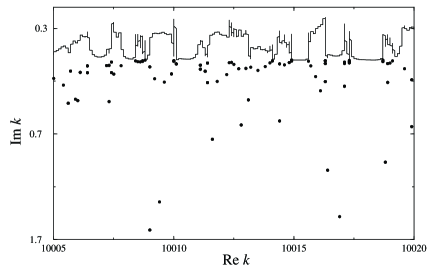
Figure 6: Quantum scattering resonances (dots) and transmission probability amplitude $T_{s_{8}s_{1}}$ (solid line) for the chain of Fig. 3 with $N=7$ unit cells.

The distribution $P(y)$ shows a peak at the origin (i.e. $y\simeq 0$) which grows with the number of unit cells, $N$. This behavior tells us that “bands” of resonances with small $y$ are created when we increase the size of the chain. In fact we have that, as for the resonances of one-dimensional open periodic potentials [26], we have $N-1$ resonances per band and that the bands converge as $\sim 1/N$ to the real axis when $N$ increases. This is consistent with the ballistic behavior that should be observed in the long-time limit.

On the other hand, the resonances with larger values of $y=|\mathrm{Im}\,k|$ are not arranged in a band structure and their number does not increase when we change the size $N$ of the system. In fact, these resonances are located at the same position in the complex plane for every value of $N$. Therefore we interpret such short-lived resonances as metastable states that decay without exploring the whole system.

In Fig. 8a, we superpose the resonance spectrum for chains with two different sizes. The figure shows that, for resonances with large values of $y=|\mathrm{Im}\,k|$, neither their position, nor their number change with $N$, but resonances with small values of $|\mathrm{Im}\,k|$ converges to the real axis as we increase $N$. Therefore, the relative number of resonances in the tail of the distribution decreases as compared to the number of resonances with small values of $y$ which increases with $N$. We can conclude that the resonance spectrum converges to the real axis in probability when we increase $N$. This behavior is in contrast with the simple systems analyzed in Ref. [26], for which we observed that each resonance converges to the real axis as $N$ increases.

Eq.(65) predicts a relative decrease of $P(y)$ as $1/N$. This law is verified as shown in Fig. 7 where we plot for clarity the function $N\times P(\mathrm{Im}\,k)$ for only a few cases. According to the theoretical distribution of Eq.(65) $N\times P(\mathrm{Im}\,k)\propto\sqrt{D}|\mathrm{Im}\,k|^{-3/2}$, where the right-hand side is independent of $N$ and moreover, the proportionality factor is determined by the diffusion coefficient of the chain. We have computed the diffusion coefficient for this graph in Ref. [9]. The continuous straight line in Fig. 7 corresponds to the diffusion coefficient of the infinite chain. The good agreement shows that the proportionality constant $a$ in Eq. (65) is of order one, as expected.

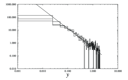
Figure 7: Superposition of the log-log plots of $N\times P(|\mathrm{Im}\,k|)$ as a function of $y=|\mathrm{Im}\,k|$ for $N=5,6,8$ and the same graph as in Fig. 3.

In Fig. 5, we observe deviations from the power law at small and large values of $|\mathrm{Im}\,k|$. The dashed lines in Fig. 5 indicate the value corresponding to the classical escape rate. We see from the figure that the distribution of imaginary parts is well described by the power law for $y=|\mathrm{Im}\,k|>\gamma_{\rm cl}/2$ and the classical escape rate $\gamma_{\rm cl}$ is near the transition to this power law. On the other hand, the tail of the distribution also deviates from the power law. The distribution follows the power law until a value which decreases when $N$ increases. Beyond this value the distribution seems to fluctuate around an almost constant value, and then drops rapidly to zero.

The region where the distribution of imaginary parts fluctuates around some value corresponds to the region where the resonances are independent (in number and in position) of the value of $N$. This can be seen in Fig. 8. In Fig. 8a, we depict the resonances for $N=7$ and $N=8$ and we draw a line which separate resonances that belongs to bands and change with $N$ from those that are independent of $N$. This line is given by $y=|\mathrm{Im}\,k|=0.5$. In Fig. 8b, we depict the density of resonances for $N=7$, the value $y=|\mathrm{Im}\,k|=0.5$ is indicated by the vertical straight line. This line marks the separation between both families of resonances and thus the limit of the power law $y^{-3/2}$.

Figure 8: (a) Resonances for the chain of Fig. 3 with $N=7$ (circles) and $N=8$ (crosses). (b) The distribution of resonance widths for the chain with $N=7$. The straight line in figure (a) and (b) separates the two families of resonances: those which depend on $N$ from those which do not. This figure shows that the change in the distribution of the imaginary parts of the resonances is associated with the different families of resonances.

7.4 Linear graph with emerging diffusion

For extended periodic open graphs, the classical decay given by the leading Pollicott-Ruelle resonance, corresponds to the decay of a diffusion process [9]. Here, we analyze the decay of the quantum staying probability for such a graph.

Here, we consider a linear periodic graph with a unit cell composed by two bonds $a$ and $b$ of incommensurate lengths $l_{a}$ and $l_{b}$, respectively. At the vertex that join these two bonds we have a scattering matrix $\sigma(\eta_{2})$ and the vertices that join two unit cells have a scattering matrix $\sigma(\eta_{1})$. These scattering matrices are of the form

$$\sigma(\eta)=\left[\begin{array}[]{cc}i\sin\eta&\cos\eta\\ \cos\eta&i\sin\eta\end{array}\right]$$ (70)

Therefore, the transmission and reflection probabilities for the classical dynamics are $T_{i}=\cos^{2}(\eta_{i})$ and $R_{i}=\sin^{2}(\eta_{i})$.

Fig. 9 depicts an open graph by considering only $N$ units cells connected to semi-infinite leads at the left-hand and right-hand side of the finite graph.

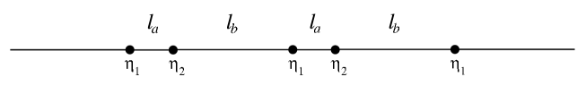
Figure 9: Open graph built out of a periodic linear chain with a unit cell made of two bonds with scattering matrices (70) at each vertex. The figure shows a chain with $N=2$ unit cells.

7.4.1 Classical diffusive behavior

In the limit $N\to\infty$ of an infinitely extended chain, the graph becomes periodic and the motion is diffusive. The diffusion coefficient can be calculated by considering the Frobenius-Perron-type matrix ${\mathsf{Q}}(s,q)$ defined in Ref. [9] in terms of the classical wavenumber $q$ and the rate $s$. For the present graph, we have that

$${\mathsf{Q}}(s,q)=\left[\begin{array}[]{cccc}0&e^{+iq}e^{-s\frac{l_{b}}{v}}T_{1}&e^{-s\frac{l_{a}}{v}}R_{1}&0\\ e^{-s\frac{l_{a}}{v}}T_{2}&0&0&e^{-s\frac{l_{b}}{v}}R_{2}\\ e^{-s\frac{l_{a}}{v}}R_{2}&0&0&e^{-s\frac{l_{b}}{v}}T_{2}\\ 0&e^{-s\frac{l_{b}}{v}}R_{1}&e^{-iq}e^{-s\frac{l_{a}}{v}}T_{1}&0\end{array}\right]$$ (71)

where the columns and rows are arranged in the following order $(a,b,\hat{a},\hat{b})$. The diffusion coefficient is obtained from the second derivative of the first branch at $q=0$. Developing $\det[{\mathsf{I}}-{\mathsf{Q}}(s,q)]$ for small values of $q$ and $s$ we get

$$\det[{\mathsf{I}}-{\mathsf{Q}}(s,q)]=2l(R_{1}T_{2}+T_{1}R_{2})\frac{s}{v}+T_{1}T_{2}q^{2}+{\cal O}(s^{2})+{\cal O}(sq^{2})+{\cal O}(q^{4})$$

The diffusion coefficient $D$ is thus given by

$$D=-\left.\frac{1}{2}\frac{\partial^{2}s_{0}(q)}{\partial q^{2}}\right|_{{\bf q}=0}=\frac{vT_{1}T_{2}}{2l(R_{1}T_{2}+T_{1}R_{2})}$$ (72)

where $l=l_{a}+l_{b}$ is the total length of the unit cell.

In Ref. [9], we have considered other examples and we have shown that the classical escape rate $\gamma_{\rm cl}(N)$ for a finite open chain of size $N$ is well approximated by Eq. (53) in the limit $N\rightarrow\infty$. For the present linear graph, Fig. 10 illustrates that the classical lifetimes of the chain are indeed determined by the diffusion coefficient according to $\tau_{\rm cl}=1/\gamma_{\rm cl}\sim N^{2}$ in the limit $N\to\infty$.

Figure 10: Plot of the lifetime $\tau_{\rm cl}(N)=1/\gamma_{\rm cl}(N)$ for the chain of Fig. 9 with $N=1$, $2$, $3$ and $4$ unit cells as a function of $N^{2}$. The dashed line corresponding to the diffusion coefficient $D=0.506v$ given by Eq.(72) is approached by the classical lifetimes for increasing size $N$ of the open graphs. We have used the parameters $\eta_{1}=0.1$ and $\eta_{2}=(\sqrt{5}-1)/2$ and $l_{a}=0.5$ and $l_{b}=\sqrt{2}$.

7.4.2 Spectrum of scattering resonances and its gap

The resonance spectrum is depicted in Fig. 11 for different chain sizes $N=1$, $2$, $3$, and $4$.

Figure 11: Scattering resonances of the chain of Fig. 9 with $N=1$, $2$, $3$ and $4$ unit cells. We have used the parameters $\eta_{1}=0.1$ and $\eta_{2}=(\sqrt{5}-1)/2$ and $l_{a}=0.5$ and $l_{b}=\sqrt{2}$.

The structures of the resonance spectrum and the presence of a gap for the sizes $N=1$ and $N=2$ can be understood thanks to the topological pressure plotted in Fig. 12 for these graphs. We see that the chains with $N=1$ and $N=2$ unit cells has a value $\tilde{P}(1/2)<0$ and, therefore, a gap empty of resonances. This gap appears in Figs. 11a and 11b. For the chains with $N=3$ and $N=4$ unit cells, $\tilde{P}(1/2)>0$ and we do not have this upper bound for Figs. 11c and 11d.

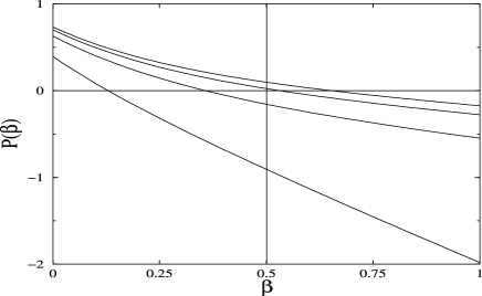
Figure 12: From bottom to top, we plotted the topological pressure for the chain of Fig. 9 with the same parameter values as in Fig. 11 and the sizes $N=1$, $2$, $3$ and $4$ unit cells, respectively.

7.4.3 Decay of the quantum staying probability

For these open graphs, we have calculated the quantum staying probability in order to illustrate the emergence of a diffusive behavior.

The quantum time evolution has been computed by using the method described in Subsection 5.4. The propagator was calculated by fast Fourier transform from the Green function. The staying probability was calculated by considering an initial Gaussian wave packet located on a bond $1$ inside the graph:

$$\psi_{1}(y,0)=\left[\sqrt{\frac{2}{\pi}}\frac{1}{\sigma(1-e^{-2\bar{E}\sigma^{2}})}\right]^{1/2}\sin(\sqrt{\bar{E}}y)e^{-\frac{(y-y_{0})^{2}}{4\sigma^{2}}}$$

This wave packet is built by the modulation of a Gaussian with a sine function of wavenumber $\sqrt{\bar{E}}$. The wave packet is thus centered at $y=y_{0}$ (and we take $y_{0}=l_{1}/2$). The wave packet is effectively on the bond 1 if $\Delta y=2\sigma<<l_{1}$.

In Fig. 13, we compare the decay of the quantum staying probability with the decay obtained from the leading Pollicott-Ruelle resonance for different sizes $N$ (see Fig. 10). This leading Pollicott-Ruelle resonance is the classical escape rate $s_{0}=-\gamma_{\rm cl}(\bar{v})$ at the velocity corresponding to the mean energy $\bar{E}$ of the Gaussian wave packet. The agreement observed in Fig. 13 for short times between the classical decay and the quantum decay shows that for short times, the quantum evolution follows a diffusion process.

The deviation that appears in Fig. 13 for longer times corresponds again to the decay determined from an isolated resonance and is therefore a pure quantum effect.

Figure 13: From bottom to top: Decay of the quantum staying probability for the chain of Fig. 9 with 1,2,3 and 4 unit cells and the same parameter values as in Fig. 11. The straight lines gives the corresponding classical decay as obtained from the Pollicott-Ruelle resonances.

8 Conclusion

We have studied dynamical and spectral properties of open quantum graphs with emphasis in their relation to the transport properties of the corresponding classical dynamics. The classical dynamics has been obtained as the classical limit of the quantum dynamics.

The time evolution of the quantum system is obtained from the propagator which is computed as the Fourier transform of the Green function. A closed expression and a multi-scattering representation for the Green function has been presented. We want to emphasize that both, classical and quantum evolution are considered with the continuous time in opposition to the discrete time evolution often considered in the literature of lattice networks.

In particular, we have computed the quantum staying probability. For short times, this quantity decay exponentially in time with the classical escape rate. This classical escape rate is obtained from the classical zeta function and correspond to the leading Pollicott-Ruelle resonance. For large open periodic graphs the leading Pollicott-Ruelle resonance determines a decay dominated by diffusion and the decay of the quantum staying probability reveals at the quantum level the emerging diffusion process.

On the other hand, the quantum spectral properties are also related to transport. The resonance spectrum reveals some features related to both, the ballistic propagation in the periodic system for the long time evolution and the diffusive classical dynamics that is an approximation for the quantum dynamics for times shorter than the Heisenberg times.

Indeed, the Fourier transform relates the long-time behavior to the variations at small energy scales. At small scales, the resonance spectrum is arranged in bands of $N-1$ resonances that converges as $\sim 1/N$ towards the real axis. Therefore the lifetime of each resonance in a band is proportional to the size of the system reflecting the ballistic transport that characterize periodic system as state the Bloch theorem [26].

Nevertheless, this ballistic propagation affects the long-time dynamics. Indeed, the Bloch theorem gives information about stationary states. The short time dynamics is determined by the large fluctuations of the resonance spectrum. At a large scale, the resonance spectrum is uniform over the $\mathrm{Re}\,k$ axis (see Fig. 4). This distribution display a power law $P(y)\sim y^{-3/2}$ early obtained in Ref. [12] and conjectured to be a general law for open quantum systems with diffusive classical limit. Our numerical results support this conjecture for multiconnected spatially extended graphs.

Moreover, we have presented an alternative derivation of the density of resonances obtained in Ref. [16], which is based on general properties of the secular equations, namely, that is an almost-periodic function which in the appropriate limit its mean motion is in the Lagrangian case. This method allows us to obtain an approximate lower bound for the distribution of $y=|\mathrm{Im}\,k|$. Moroever, an upper bound for this distribution has been obtained from the topological pressure $\tilde{P}(\beta)$. This bound creates a gap in the resonance spectrum under the condition $\tilde{P}(1/2)<0$ and is absent otherwise.

In summary, we have studied quantum properties of extended open periodic graphs. We have shown that the Pollicott-Ruelle resonances determine the decay of the quantum staying probability, which in turn shows the appearance of diffusion at the quantum level. The diffusion process is thus encoded in the distribution of scattering resonances.

References

- [1] P. Gaspard, Chaos, Scattering and Statistical Mechanics (Cambridge University Press, Cambridge UK, 1998).
- [2] T. Kottos and U. Smilansky, Phys. Rev. Lett. 79, 4794 (1997).
- [3] T. Kottos and U. Smilansky, Annals of Physics 273, 1 (1999).
- [4] H. Schanz and U. Smilansky, Philos. Mag. B 80 1999 (2000).
- [5] G. Berkolaiko and J. P. Keating, J. Phys. A: Math. & Gen. 32, 7827 (1999).
- [6] F. Barra and P. Gaspard, J. Stat. Phys. 101, 283-319 (2000); quant-ph/0011098.
- [7] E. Akkermans, A. Comtet, J. Desbois, G. Montambaux, and C. Texier, Annals of Physics 284, 10 (2000).
- [8] H. Schanz and U. Smilansky, Phys. Rev. Lett. 84, 1427 (2000).
- [9] F. Barra and P. Gaspard, Phys. Rev. E 63, 066215 (2001); nlin.CD/0011045.
- [10] G. Casati, G. Maspero, and D. L. Shepelyansky, Phys. Rev. E 56, R6233 (1997).
- [11] K. Pance, W. Lu, and S. Sridhar, Phys. Rev. Lett. 85, 2737 (2000).
- [12] F. Borgonovi, I. Guarneri, and D. L. Shepelyansky, Phys. Rev. A, 43, 4517 (1991).
- [13] J. Avron, A. Raveh, and B. Zur, Rev. Mod. Phys. 60, 873 (1988).
- [14] P. Exner and P. Seba, Rep. Math. Phys. 28 7 (1989).
- [15] P. Exner and P. Seba, Phys. Lett. A 128 493 (1988).
- [16] T. Kottos and U. Smilansky, Phys. Rev. Lett. 85, 968 (2000).
- [17] R. Balian and C. Bloch, Annals of Physics 60, 401 (1970).
- [18] P. Gaspard and S. A. Rice, J. Chem. Phys. 90, 2225, 2242, 2255; 91, E3279 (1989).
- [19] P. Gaspard, in: G. Casati, I. Guarneri, and U. Smilansky, Editors, Quantum Chaos (North-Holland, Amsterdam, 1993) pp. 307-383.
- [20] P. Gaspard, D. Alonso, and I. Burghardt, Adv. Chem. Phys. 90, 105 (1995).
- [21] P. Gaspard and I. Burghardt, Adv. Chem. Phys. 101, 491 (1997).
- [22] P. Gaspard, in: J. Karkheck, Editor, Dynamics: Models and Kinetic Methods for Nonequilibrium Many-Body Systems (Kluwer Academic Publishers, Dordrecht, 2000) pp. 425-456.
- [23] J. Sjöstrand, Duke Math. J. 60, 1 (1990).
- [24] M. Zworski, Invent. Math. 136, 353 (1999).
- [25] K. K. Lin and M. Zworski, Quantum Resonances in Chaotic Scattering (preprint, University of California at Berkeley, 2001).
- [26] F. Barra and P. Gaspard, J. Phys. A: Math. & Gen. 32 5852 (2000).
- [27] B. Jessen and H. Tornehave, Acta Mathematica 77, 137 (1945).