Replica-symmetry breaking in dynamical glasses

Abstract

Systems of globally coupled logistic maps (GCLM) can display complex collective behaviour characterized by the formation of synchronous clusters. In the dynamical clustering regime, such systems possess a large number of coexisting attractors and might be viewed as dynamical glasses. Glass properties of GCLM in the thermodynamical limit of large system sizes $N$ are investigated. Replicas, representing orbits that start from various initial conditions, are introduced and distributions of their overlaps are numerically determined. We show that for fixed-field ensembles of initial conditions all attractors of the system become identical in the thermodynamical limit up to variations of order $1/\sqrt{N}$, and thus replica symmetry is recovered for $N\rightarrow\infty$. In contrast to this, when random-field ensembles of initial conditions are chosen, replica symmetry remains broken in the thermodynamical limit.

1 Introduction

The rich collective behaviour displayed by globally coupled logistic maps (GCLM) Kan ; Kan1 has made them to become a paradigm of complex dynamical systems. Initially, GCLM were introduced as a mean field approach to coupled map lattices. Subsequently, they have been used as metaphors of neural dynamics, ecology, and cell differentiation Kbook . Understanding the properties of GCLM can be seen as a first step towards grasping the dynamics and emergent properties of real, high-dimensional systems. The dynamical equations describing the system are

$$x_{i}(t+1)=(1-\epsilon)f(x_{i}(t))+\frac{\epsilon}{N}\sum_{j=1}^{N}f(x_{j}(t))\;$$ (1)

where

$$f(x)=1-ax^{2}$$ (2)

is the logistic map. The parameter $\epsilon\in[0,1]$ gives the strength of coupling among elements. For $\epsilon=0$ the elements evolve independently, and for $\epsilon=1$ they are synchronized already after the first iteration and follow identical trajectories ever after. Between these two extreme behaviours, a broad spectrum of collective dynamics emerges. The dynamics is strongly sensitive to the control parameter $a$ of the logistic map and depends on the size $N$ of the system. Figure 1 shows a rough phase diagram of GCLM, based on the collective behaviour of the system which is reached after (sometimes, very long) transients Kan ; MM1 ; Abramson . The diagram includes both the parameter interval $a<1.4$ where dynamics of an individual map is periodic and the interval $1.4<a<2$ with chaotic individual dynamics. It contains two large domains of synchronous and turbulent phases. They are separated by a region with glass-like behaviour. In the synchronous domain the states of all elements are identical and the ensemble has the same dynamics as a single map. In the turbulent phase, the ensemble of maps is essentially desynchronized, though nontrivial correlations have been detected even there Shibata . The glass region is characterized by the formation of various dynamical clusters.

Numerical simulations of GCLM have shown that, in the dynamical glass phase, the system displays sensitivity to initial conditions. For fixed parameters $\epsilon$ and $a$ (and given $N$), a multiplicity of attractors can be reached Kan ; Chaos . This property is similar to what is observed in glassy systems, where the presence of quenched disorder causes frustration and a large number of macroscopic configurations are possible Mezard . For this reason, GCLM have been described as a dynamical counterpart to spin glasses Kanglass , Vulpiani . In a previous publication MM2 two of us have introduced a replica description for this system, defined overlaps and numerically tested replica-symmetry breaking and ultrametric properties of GCLM. Our analysis has revealed a strong size dependence of collective dynamics, indicating that replica symmetry might be recovered in the thermodynamic limit $N\rightarrow\infty$. The aim of the present paper is to investigate systematically the asymptotic statistical properties of GCLM in this limit.

Our main result is that the asymptotic behaviour observed in the thermodynamic limit is strongly dependent on how the ensemble of initial conditions is prepared. In previous studies Vulpiani ; MM2 , the procedures used for random generation of initial conditions had a special property: in the limit $N\rightarrow\infty$ all generated initial conditions were effectively identical up to order $1/\sqrt{N}$. Therefore, all explored attractors in the glass phase became equivalent up to variations of order $1/\sqrt{N}$ and the replica symmetry was recovered in the thermodynamic limit. Now we show that, if the initial conditions are prepared in such a way that the initial field always retains macroscopic fluctuations, the replica symmetry is clearly broken in the thermodynamic limit $N\rightarrow\infty$. Thus, GCLM represent the first known example of a dynamical glass with replica-symmetry breaking and, as we show, this important statistical property does not represent a finite-size effect. Our results also imply that the boundaries between different regions illustrated in Fig. 1 depend on the ensemble of initial conditions, and that, for broad ensembles and $\epsilon$ not too large, fully synchronized attractors can coexist with multi-cluster attractors.

In the next section we introduce dynamical and statistical measures needed to characterize clustered states of GCLM. They include the splitting exponent, earlier proposed by Kaneko Ksplit , and a new repulsion exponent which we suggest. Replicas and their overlaps are defined and attraction basin weights are considered here. In Section 3 we perform a detailed analysis of the role of initial conditions. Replica symmetry breaking and ultrametric properties of GCLM in the thermodynamic limit are investigated in Section 4 under a truly random choice of initial conditions. The paper ends with a discussion of the main results, which are compared to the properties of other disordered systems.

Figure 1: Rough phase space of GCLM showing the main three phases of the system.

2 Characterization of attractors

An attractor of the dynamical system (1) is characterized by the formation of a number of clusters out of the initially symmetrical ensemble of maps. This is one of the most intriguing properties of GCLM. Within each cluster all elements are completely synchronized. A partition of $N$ maps into $\mathcal{K}$ clusters is defined by indicating the numbers $N_{k}$ of elements in each cluster, $k=1,\dots\mathcal{K}$. In the following, we assume that the clusters have been ordered such that $N_{1}\geq N_{2}\geq\dots\geq N_{\mathcal{K}-1}\geq N_{\mathcal{K}}$. Even if only two clusters are present, this can correspond for $N\rightarrow\infty$ to a huge number of different partitions, since the relative sizes of clusters may vary.

In the periodic region, and for $\epsilon=0$, the elements can be trivially classified into $N/P$ groups, where $P$ is the period of the single map, and elements within each group follow the periodic orbit of the single map with different phases. At large enough $\epsilon$ the number of simultaneously stable clusters decreases and their dynamical behavior differentiates. This happens approximately in the whole area labeled “dynamical glass” in Fig. 1. For $\epsilon$ large enough, all of the maps are synchronized and the dynamics reduces to that of the single element (synchronous phase). Note that fully synchronized attractors and multi-cluster attractors can coexist in some region of parameter space.

In the glass phase, attractors of GCLM correspond to different partitions in clusters. The global dynamics of each attractor can be periodic, quasiperiodic or chaotic. The periodic collective dynamics is by far the most common, and is typically found even in the parameter region where the dynamics of a single map is chaotic.

2.1 Splitting and repulsion exponents

The route to synchronization can be easily found by studying how the distance between elements evolves in time. This is ruled by the equation

$$x_{i}(t+1)-x_{j}(t+1)=-(1-\epsilon)a\left(x_{i}^{2}(t)-x_{j}^{2}(t)\right)\,.$$ (3)

Integrating it over a time $T$, one finds

$$\left|x_{i}(t+T)-x_{j}(t+T)\right|=\exp(T\lambda_{ij})\left|x_{i}(t)-x_{j}(t)\right|\,,$$ (4)

$$\lambda_{ij}=\ln\left(a(1-\epsilon)\right)+\frac{1}{T}\sum_{t}\ln|x_{i}(t)+x_{j}(t)|\;,$$ (5)

If two elements belong to the same cluster $b$, their distance has to shrink to zero. In this case, $x_{i}(t)\approx x_{j}(t)\approx X_{b}(t)$. Kaneko Ksplit defined the splitting exponent to measure the rate of convergence to the orbit $\{X_{b}(t)\}$,

$$\lambda_{b}=\ln\left(2a(1-\epsilon)\right)+\lim_{T\to\infty}\frac{1}{T}\sum_{t}\ln|X_{b}(t)|\;,$$ (6)

and defined an orbit as transversely stable if it has $\lambda_{b}<0$ (see also Chaos ). While in the definition of the splitting exponent the partition $N_{1}\cdots N_{\cal K}$ does not enter, it is the distribution of the elements into clusters which decides whether a set of orbits is a global attractor or not. All of the stable periodic orbits of the single map have negative splitting exponent for every positive $\epsilon$. The splitting exponent can be positive for non-entrained elements (forming “clusters” of a single element) in the chaotic domain of the logistic map.

Due to the unavoidable finite precision of digital computers, the simulation of the deterministic system (1) can lead to pseudo-attractors which are not stable against transversal perturbations. In the results to be presented, we have computed $\lambda_{b}$ for all orbits and discarded unstable attractors.

There is another condition which must be required for having a stable partition and which, to our knowledge, has not been made explicit yet. On the one hand, if two elements $i$ and $j$ belong asymptotically to two different orbits $b$ and $c$, their distances (5) should remain finite. On the other hand, since the phase space is finite, the distances cannot diverge. Thus, the orbits of the two clusters have to fulfill the condition

$$\lambda_{bc}=\ln\left(a(1-\epsilon)\right)+\lim_{T\to\infty}\frac{1}{T}\sum_{t}\ln|X_{b}(t)+X_{c}(t)|=0\;.$$ (7)

For periodic orbits, this condition is just a consequence of periodicity. Nevertheless, it allows to rationalize some features of GCLM. We call $\lambda_{bc}$ repulsion exponent, since its positive value would mean that the two orbits repel each other, and define two orbits as orthogonal if their repulsion exponent vanishes. A set of orbits is stable if all of the orbits are transversely stable and all pairs of orbits are orthogonal. This condition does not depend on the partition of the $N$ elements into the $\cal K$ orbits, but a precise partition is needed so that the set of orbits is invariant under the global dynamics.

Note that, for $\epsilon=0$, the set of all periodic orbits, stable and unstable, fulfill the orthogonality condition, which is just equivalent to periodicity. Thus, if the dynamics of the single map is periodic with period $P$, the $P$ orbits obtained from the different phases of the stable periodic orbit constitute a stable set. As $\epsilon$ increases, the transversal stability condition becomes easier to fulfill even for lower periodicity orbits, but the orthogonality condition becomes more difficult (notice that the larger the number of clusters, the more demanding this condition). Thus at some point only partitions with less than $P$ clusters can be found. This is probably a reason why only very small numbers of clusters are typically observed in simulations. Additionally, since the average value $\sum_{t}\ln|X_{b}(t)+X_{c}(t)|/T$ cannot be larger than $\log(2)$, no stable two cluster system can exist for $\epsilon>1-1/2a$. This is only an upper bound, since the actual value of $\epsilon$ where multiple cluster attractors disappear is much smaller.

In Fig. 2 we show the two splitting exponents as well as the repulsion exponent for a two-cluster system with parameters $a=1.3$ and $\epsilon=0.15$. There is a continuous spectrum of partitions allowed, and for all of them the clusters move along period-two orbits, which are periodic orbits of the two variable dynamical system

$$X_{1}(t+1)=1-a\left((1-\epsilon(1-p))X_{1}^{2}(t)+\epsilon(1-p)X_{2}^{2}(t)\right)$$

$$X_{2}(t+1)=1-a\left((1-\epsilon p)X_{2}^{2}(t)+\epsilon pX_{1}^{2}(t)\right)\,,$$ (8)

where $p=N_{1}/N$ is the fraction of elements in the largest cluster and is kept fixed during the dynamics. Notice that the repulsion exponent $\lambda_{12}$ equals zero up to very high precision for all values of $p$. For these parameter values also the completely synchronized state is stable, and moves along a period-four attractor whose attraction basin covers roughly 70% of phase space for the values of $p$ where the two clusters are stable. At large $p$, the transversal exponent $\lambda_{2}$ approaches zero, and the two-orbit system becomes unstable while the synchronized attractor covers 100% of phase space.

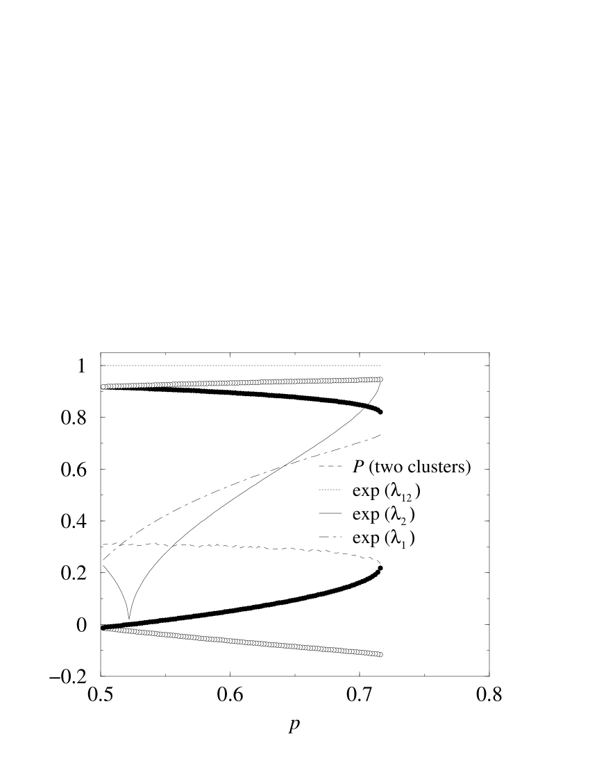
Figure 2: Possible two-cluster partitions for a system with $a=1.3$ and $\epsilon=0.15$. For different values of the relative size $p$ of the largest cluster the two clusters move along two period-two orbits represented as empty and solid circles, respectively. The fraction of initial conditions converging to two-cluster orbits is shown as a dashed line. The remaining trajectories synchronize completely to the stable period-four orbit. The two transversal exponents $\lambda_{1}$ and $\lambda_{2}$ as well as the repulsion exponent $\lambda_{12}$ are shown. Notice that $\lambda_{1}$ attains a minimum at $p\simeq 0.52$. Empty circles represent the first period two orbit, full circles represent the second one.

2.2 Replicas and overlaps

In MM2 , two of us have introduced the concept of replica in GCLM and a measure of similarity between them, the overlap $q^{\alpha\beta}$. A replica $\alpha$ is an orbit $\{x_{i}^{\alpha}(t)\}$ of the whole system, and different replicas are obtained from different realizations of the initial conditions. Thus, the overlap $q_{\alpha\beta}$ is a random variable dependent on the sets of initial conditions $\{x_{i}^{\alpha}(0)\}$ and $\{x_{i}^{\beta}(0)\}$. We investigate its distribution for specific ensembles of initial conditions, keeping the parameters $\epsilon$, $a$, and $N$ fixed.

In order to compute the overlap, we transform the orbits into binary sequences, assigning a binary number $\sigma_{i}(t)$ to each element $i$ at each time step $t$ such that $\sigma_{i}^{\alpha}(t)=1$ if $x_{i}^{\alpha}(t)>x^{*}$, and $\sigma_{i}^{\alpha}(t)=-1$ otherwise, with

$$x^{*}=\frac{-1+\sqrt{1+4a}}{2a}$$ (9)

the fixed point of a single logistic map.

Finally, the overlap $q^{\alpha\beta}$ is defined as

$$q^{\alpha\beta}=\frac{1}{NT}\sum_{t=t_{0}}^{t_{0}+T}\sum_{i=1}^{N}\sigma_{i}^{\alpha}(t)\sigma_{i}^{\beta}(t)\;.$$ (10)

This quantity is computed after a large enough transient time $t_{0}$ has elapsed, so that the two trajectories reach their asymptotic attractors, and averaged over the minimal common multiple of the two periods or, in case the asymptotic dynamics is not periodic, over a very large simulation time $T\simeq 10^{2-4}$, depending on the underlying dynamics. The overlap takes values between -1 and 1. In order for it to be a meaningful measure of similarity, the value 1 should be returned if and only if the two asymptotic attractors coincide. Even in this case, however, the above formula can take different values depending on the relative phase of the two orbits and on the permutation of elements. To avoid this, the second orbit is shifted by a number time steps with respect to the first one in order to maximize the overlap. This procedure is similar to that used in spin glasses with rotational symmetry Fischer . Finally, the degeneracy due to the arbitrary initial labelling can be avoided through a proper reordering of the elements once the stable attractor has been reached: Elements in the largest cluster are assigned labels from $1$ to $N_{1}$, those in the second largest from $N_{1}+1$ to $N_{1}+N_{2}$, and so on.

Using the previous definition, the overlap $q$ returns a finite positive value for clusters of periodic orbits and of chaotic ones in the two-band chaos, due to the regular alternation of plus one and minus one values in this region. Orbits with one-band chaos change the sign of the sequence $\sigma(t)$ in an uncorrelated fashion, implying that in the limit $T\to\infty$ their overlap with other orbits tends to zero. Our numerical simulations indeed show that this is the case. Thus, the definition of the overlap becomes problematic for orbits with one-band chaos.

2.3 Attraction basin weights

The overlap distribution gives information on the distribution of attraction basin weights for the particular ensemble of initial conditions chosen. In fact, we can write it as

$$P(q)=\sum_{\alpha\beta}W_{\alpha}W_{\beta}\delta(q-q_{\alpha\beta})\;,$$ (11)

where $\alpha$ and $\beta$ label all possible global attractors, $q_{\alpha\beta}$ is their overlap, and $W_{\alpha}$ and $W_{\beta}$ are their attraction basin weights, i.e. the fraction of initial conditions which converge to the attractors $\alpha$ and $\beta$ respectively, and whose sum is normalized to unity. The overlap distribution contains a delta distribution at $q=1$, obtained for $\alpha=\beta$, whose size is equal to the average attraction basin weight:

$$Y=\sum_{a}W_{a}^{2}\;.$$ (12)

This parameter expresses the probability that two randomly chosen initial conditions converge to the same attractor and is able to distinguish between different situations. If $Y$ is equal to or tends to one in the thermodynamic limit, it means that there is only one relevant attractor which attracts in this limit all of the phase space of the system. If $Y$ tends to zero in the thermodynamic limit, it means that the system has in this limit a diverging number of different attractors and none of them is dominant. The situation in between, when $Y$ is finite but smaller than one, means that there is a finite number of relevant attractors.

For a fixed value of $a$ and increasing $\epsilon$, the collective behaviour of GCLM changes from turbulent to glassy (multiple clusters) to finally fall into complete synchronization. This last transition can be characterized through different parameters. Kaneko proposed to use the average cluster number Kan , which grows continuously from a finite value in the dynamical glass phase to unity in the synchronous phase (for fixed $N$). An alternative measure can be the fraction $W_{\mathrm{CS}}$ of initial conditions converging to the single coherent attractor. It turns out that multiple-cluster attractors have vanishing attraction basins in the thermodynamic limit, so that the only nonvanishing contribution to $Y$ comes from the completely synchronized attractor, and we can approximate $Y\simeq W_{\mathrm{CS}}^{2}$. Thus we can also study through the parameter $Y$ the transition between complete and partial synchronization.

3 Fixed-field ensemble

To compute overlap distributions and other statistical properties of GCLM, a set of replicas corresponding to different initial conditions should be taken. Ideally, all initial conditions should be present in the set. In an actual computation, this is never possible. Instead, a large ensemble of initial conditions is randomly generated. One expects that averaging over this ensemble would be equivalent to the ideal averaging over “all” initial conditions. However, this would only be true if the employed random set is relatively uniformly sampling the full space of initial conditions. Some random sets of initial conditions may be missing this property. In previous numerical investigations Vulpiani ; MM2 of dynamical glasses, to generate a set of initial conditions the coordinate $x_{i}(0)$ of each map $i=1,...,N$ was chosen independently and with a uniform probability density from the interval $(-1,1)$. It was tacitly assumed that this procedure would yield uniform sampling of initial conditions. However, the initial conditions generated in this way become increasingly similar in the thermodynamic limit $N\to\infty$.

As follows from (1) and (2), the dynamics of GCLM is described by the equations

$$x_{i}(t+1)=1-a\left[(1-\epsilon)x_{i}^{2}(t)+\epsilon m(t)\right]$$ (13)

where

$$m(t)=\frac{1}{N}\sum_{i=1}^{N}x_{i}^{2}(t)$$ (14)

is the synchronizing field that acts on a given element $i$ and is collectively produced by the whole system.

Let us consider statistical properties of the initial synchronizing field $m=m(t=0)$ in the limit of large $N$, when the coordinates $x_{i}(0)$ of each map $i=1,...,N$ are chosen independently and with a uniform probability density from the interval $(-1,1)$. Because this field represents then a sum of a large number of independent random variables, it should obey for $N\to\infty$ a Gaussian probability distribution

$$p(m)=\frac{1}{\sqrt{2\pi\sigma}}\exp\left[-\frac{\left(m-\overline{m}\right)^{2}}{2\sigma}\right]$$ (15)

where $\overline{m}$ is the mean value of the field $m$ and $\sigma$ is its mean-square statistical variation. Using (14), we obtain

$$\overline{m}=\frac{1}{N}\sum_{i=1}^{N}\langle x_{i}^{2}(0)\rangle=\frac{1}{2N}\sum_{i=1}^{N}\int_{-1}^{1}x^{2}dx=\frac{1}{3}$$ (16)

and

$$\sigma=\langle(m-\overline{m})^{2}\rangle=\frac{1}{N^{2}}\sum_{i=1}^{N}(\langle x_{i}^{4}(0)\rangle-\langle x_{i}^{2}(0)\rangle^{2})=\frac{4}{45N}$$ (17)

Thus, in the thermodynamic limit $N\to\infty$ the initial synchronizing field approaches a constant value, independent of the realization. For large $N$’s it shows fluctuations of order $1/\sqrt{N}$. Such a set of initial conditions shall be called a fixed-field ensemble below.

Below in this section we discuss glass properties of GCLM for evolutions starting from a fixed field ensemble (to our knowledge, this is the only way in which the initial conditions have been so far modelled in the literature). As we shall see, this ensemble leads to replica symmetry, since all approached attractors are then identical up to small variations which vanish in the thermodynamic limit.

3.1 Transition to complete synchronization

At sufficiently high coupling strength $\epsilon$, GCLM become completely synchronized. We characterize the transition to complete synchronization through the probability $Y=P(q=1)$ (see Eq. (12)) that two randomly chosen initial conditions from a fixed-field ensemble fall into the same attractor, see Fig. 3. Our analysis is performed with a value of the logistic parameter $a=1.3$ where the single logistic map is periodic with period four. The coexistence of different attractors and their dynamics for this parameter choice have been previously considered in Chaos . Near the transition to complete synchronization the final stable attractors consist of two clusters following the dynamics of period two.

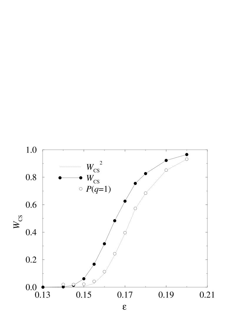
Figure 3: Transition to complete synchronization. When coupling $\epsilon$ is increased, the attraction basin of the completely synchronous state grows until all initial conditions end there.

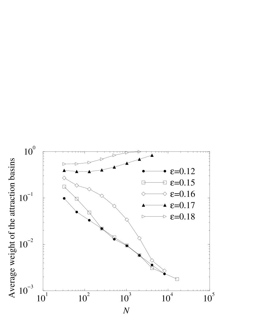
Figure 4: Average weight of an attractor basin $Y=P(1)$ as a function of the system size for $a=1.3$.

It is interesting how this transition takes place in the thermodynamic limit. Each curve in Fig. 4 represents $Y$ for a given value of $\epsilon$ as a function of $N$. Even if the completely synchronized state is stable for $\epsilon>\epsilon_{1}(a)$, the smallest value at which the synchronized state is transversally stable, this state is never observed until $\epsilon$ reaches a larger value $\epsilon>\epsilon_{2}(a)$ Chaos . The transition is discontinuous (first order) and takes place at $\epsilon\simeq 0.165$ for $a=1.3$. For smaller $\epsilon$ the system is in a phase where many different attractors coexist. All of them are two-cluster attractors. Since the average attraction basin weight $Y$ vanishes in the thermodynamic limit, the number of different attractors diverges for $N\rightarrow\infty$. The unbounded increase of the number of different attractors for $N\to\infty$ was indeed one of the first indications that GCLM might represent a glass-like system Vulpiani .

We have further examined how the number of attractors $\mathcal{M}$ visited by the system grows as the number $\mathcal{I}$ of different initial conditions used increases. Our results for $\epsilon=0.15$ and $a=1.3$ are displayed in Fig. 5. We observe an approximate power-law dependence $\mathcal{M}\propto\mathcal{I}^{\eta}$, with an exponent $\eta$ dependent on the system size $N$. For $\mathcal{I\to\infty}$, $\mathcal{M}$ should saturate at a finite value. Although the number of different attractors grows fast, the bending at large $\mathcal{I}$ for the largest size reflects the existence of an asymptotic value $\mathcal{\ M}_{\infty}(N)$.

Figure 5: The number of different attractors reached by the system increases as a power law of the number of random initial conditions used. Increasing the latter number is equivalent to exploring in higher detail the phase space. From top to bottom, $N=16384$, $4096$, $1024$, and $256$.

3.2 Distributions of overlaps

Figure 6: Data collapse of the normalized overlap distribution under increasing system size; system parameters $\epsilon=0.15$ and $a=1.3$.

To quantify the similarity between different attractors, we have calculated the overlap distributions for the same parameters, $\epsilon=0.15$ and $a=1.3$, and different system sizes $N$. As seen in Fig. 6, such distribution $P(q)$ approaches a delta-function in the thermodynamic limit $N\rightarrow\infty$. The width of the main peak in $P(q)$ goes to zero as $1/\sqrt{N}$. Some finite-size effects can be observed in the bump at the smallest size represented, and in the peaks which appear intermittently for relatively large values of $N$, showing the “locking” of the system close to prefered partitions, before reaching the asymptotic behaviour.

The finite-size behaviour can also be more complicated. Fig. 7 shows the overlap distributions obtained at the same control parameter $a=1.3$ for four different values of $\epsilon$ and systems of size $N=256$. For small $\epsilon$ (Fig. 7a), there is a large number of partititions close to the attractor with the largest basin, $N_{1}=149$, $N_{2}=107$. A second group of attractors corresponds to three-cluster families close to $N_{1}=115$, $N_{2}=85$, $N_{3}=55$. The attractors within each group are similar and their mutual overlaps are close to unity, explaining the large weight of $P(q)$ at $q\simeq 1$. The overlaps between these two groups give a second contribution around $q=0.7$. The continuous line in Fig. 7a shows the total distribution, the dashed line corresponds to the attractors with the same number of clusters, and the dotted line represents the contribution from the overlaps between two- and three-cluster attractors. The part of the distribution close to $q=1$ results from three-cluster attractors where the third cluster has only a few elements. As the coupling strength grows, the three-cluster attractors become less and less frequent, and two-cluster attractors dominate (Fig. 7b,c). For large enough coupling (an example is $\epsilon=0.17$ in Fig. 7d), the completely synchronous state appears and starts to occupy an increasingly large fraction of the phase space. Its self-overlap is unity, while its overlap with the remaining two-cluster attractors is small (three-cluster attractors are no longer present). The overlap between one- and two-cluster attractors explains the large contribution at small values of $q$ observed in Fig. 7d. If $\epsilon$ increases further, the completely synchronous state attracts more and more initial conditions, $P(q)$ tends to a delta-function at $q=1$, and the contribution at small $q$ disappears.

Figure 7: Overlap distributions for $N=256$ and $a=1.3$. (a) $\epsilon=0.05$, (b) $\epsilon=0.1$, (c) $\epsilon=0.14$, and (d) $\epsilon=0.17$.

In the chaotic domain of a single logistic map, for $a>a_{\infty}$, a similar behavior but with strong finite-size effects is observed. In a previous publication MM2 , we have studied the parameters $\epsilon=0.1$ and $a=1.55$. This point had been also analysed in Vulpiani for its glassy properties. The overlap distribution is broad here and its shape keeps almost unchanged with the system size until $N\simeq 4000$. But when $N$ increases further, the most of the distribution’s weight is shifted towards $q\simeq 1$, indicating that the attractors reached by the system indeed become very similar. For $\epsilon=0.3$ and $a=1.9$, we have observed that for sizes up to $N\simeq 3000$, the overlap distribution $P(q)$ remains almost constant (see Fig. 4 in MM2 ). If we apply rescaling similar to Fig. 6, only the two largest sizes ($N=2048$ and $N=8192$) seem to follow the expected asymptotic behaviour and collapse.

Our analysis shows that, for $N$ large enough, GCLM tend to a prefered cluster partition. It can be said that the same macroscopic state is always found in the thermodynamic limit, apart from “thermal fluctuations” of order $1/\sqrt{N}$. The origin of such fluctuations lies in the $1/\sqrt{N}$ variations of the synchronizing field.

3.3 Distributions of cluster sizes

Information similar to the overlap distribution is contained in the distribution $Q(p_{k})$ of cluster sizes $p_{k}=N_{k}/N$, i.e. of the fractions of elements belonging to a cluster (obviously, $\sum_{k}p_{k}=1$). For large sets of initial conditions (varying between $10^{4}$ and $2\times 10^{5}$ realizations) in the fixed-field ensemble, we have computed the values of $p_{k}$ for all stable partitions and thus obtained the distributions $Q(p_{k})$ of cluster sizes.

An example of such distributions for $\epsilon=0.15$ and $a=1.3$ and different system sizes is shown in Fig. 8a. We see that in this case the asymptotic attractors are always formed by two clusters of unequal size. Their dynamics is periodic with period two. As $N\to\infty$, the distribution $Q(p_{k})$ shrinks in width around the two prefered sizes, $p_{1}\simeq 0.372$ and $p_{2}=1-p_{1}$. For large enough $N$ the two peaks approach a Gaussian distribution, and its width decreases proportional to $1/\sqrt{N}$ , as shown in Fig. 8b.

Figure 8: (a) Distribution of cluster sizes for increasing system size; parameters $\epsilon=0.15$ and $a=1.3$. (b) Data collapse of the size distribution for the largest cluster, with $N_{1}\simeq 0.628N$.

A similar behaviour was observed for other parameter values. Generally, for sufficiently large $N$ the distribution of the sizes of the $k$th cluster is a Gaussian centered at a prefered value $p_{k}^{*}$. We show two more examples. In Fig. 9a ($\epsilon=0.3$ and $a=1.9)$, the system tends to attractors with two clusters of almost equal sizes, though occasionally also three-cluster attractors are observed. Fig. 9b ($\epsilon=0.1$ and $a=1.55$) gives an example where attractors with four clusters of different sizes are prefered. We show the total size distribution $Q(p_{k})$ together with the size distributions for clusters of rank one to four. Here, the prefered partition is close to $p_{1}=0.307$, $p_{2}=0.242$, $p_{3}=0.2295$, and $p_{4}=0.2215$.

Thus, we have investigated numerically the statistical properties of GCLM in the glass phase starting from initial conditions in the fixed-field ensemble. The investigations show that in the thermodynamic limit $N\rightarrow\infty$ this system has a great number of different attractors, increasing as a power law of system size $N$. However, all these attractors are very similar. Namely, the differences in their statistical properties, such as the cluster sizes, are proportional to $1/\sqrt{N}$ and thus vanish in the limit $N\rightarrow\infty$. This explains why replica-symmetry is recovered in the thermodynamic limit, when only the evolutions initiating from a fixed-field ensemble are considered.

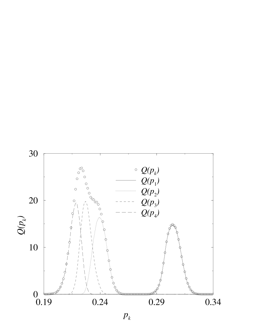
Figure 9: (a) Distribution of cluster sizes for different system sizes, $\epsilon=0.3$, and $a=1.9$. For $N$ large enough, the system chooses a partition formed by two clusters of similar sizes. (b) Distribution $Q(p_{k})$ for $N=8192$ and parameters $\epsilon=0.1$ and $a=1.55$. The whole distribution $Q(p_{k})$ and individual distributions for the largest, second, third, and fourth largest clusters are displayed.

4 Random-field ensemble

4.1 The role of initial conditions

For given parameter values $a$ and $\epsilon$, many different orbits corresponding to a continuous spectrum of two-cluster partitions and to complete synchronization are stable (see Fig. 2). Yet, only one partition is chosen in the fixed-field ensemble, up to variations of order $1/\sqrt{N}$. The selection of this prefered partition cannot be explained by a higher stability of its orbit. For instance, Fig. 2 indicates that for $a=1.3$ and $\epsilon=0.15$ the transversal stability is strongly increased at the cluster size $p_{1}\simeq 0.522$. However, the selected partition in the fixed-field ensemble has in this case the cluster size $p_{1}=0.628$ whose stability is much weaker. For parameters in the chaotic domain of a single logistic map, the situation is similar. Stable attractors with chaotic dynamics exist here, but the system often shows a preference for the periodic ones.

To examine in more detail the role of initial conditions, we use a slightly generalized version of the fixed-field ensemble. Namely, we assume now that the initial coordinates $x_{i}(0)$ of all maps are independently and uniformly distributed between $-\xi$ and $\xi$ (note that the fixed-field ensemble corresponds then to the choice $\xi=1$). Calculating again the statistical distribution of initial synchronizing fields $m$, we find that in the thermodynamic limit $N\rightarrow\infty$ it is again given by a Gaussian distribution with mean value $\overline{m}=\xi/3$ and mean-square dispersion $\sigma=(4/45)(\xi/N)$. Hence, at time $t=1$ the coordinates $x_{i}(1)$ of the maps are given by

$$x_{i}(1) = 1-a\left[(1-\epsilon)x_{i}^{2}(0)+\epsilon m\right]$$ (18)

$$= 1-a\left[(1-\epsilon)x_{i}^{2}(0)+\epsilon{\frac{\xi}{3}}+O(N^{-1/2})\right]\;.$$

Since $x_{i}(0)$ is uniformly distributed, $x_{i}^{2}(0)$ is distributed with density $1/2x$ which diverges at $x_{i}^{2}(0)=0$, so that the distribution of $x_{i}(1)$ has a pronounced maximum at $x=1-a\epsilon\xi/3$ . This initial bias drives the system towards the attractor closest to the most probable value of $x_{i}(1)$. This is shown in Fig. 10, where we represent, as a function of the fixed ensemble parameter $\xi$, the value $1-a\epsilon\xi/3$ where the maximum of $x_{i}(1)$ is expected, the actually observed maxima of $x_{i}(1)$, and the coordinate on the prefered asymptotic orbit. Varying $\xi$, the bias in the initial value $x_{i}(1)$ changes and drives the system to different asymptotic orbits (full circles in Fig. 10), in turn corresponding to different partitions of the elements. We thus find $p=0.632$ at $\xi=1$ and $p=0.717$ at $\xi=0.944$. Partitions with larger $p$ cannot lead to two transversely stable orbits, thus for $\xi<0.944$ the completely synchronized attractor is always reached.

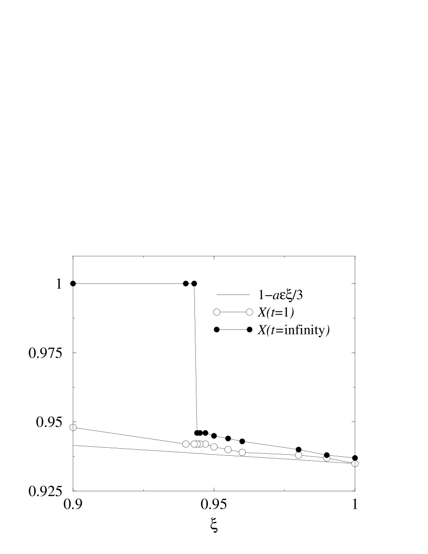
Figure 10: For different values of the initial field, the figure shows the most likely value of $x_{i}(1)$ (empty circles) and the coordinate of the prefered attractor closest to this value (full circles). For $\xi<0.944$ the prefered attractor is completely synchronized.

It is interesting, in this framework, to look at the dynamics of synchronization for $a=1.3$, $\epsilon=0.15$ and varying $\xi$ (see Fig. 11). Different examples always show the same pattern: after the first time step, the most populated region of phase space coincides with the maximum in the distribution of $x_{i}(1)$. After very few time steps, the two most populated “clusters” start to oscillate close to a stable attractor made of two periodic orbits of period two, but most elements are not synchronized yet and the partition is quite different from the final one. At the same time as oscillations around the periodic orbits are dumped, more and more elements join the two clusters, until the partition which stabilizes the periodic orbits is reached. Thus the system first chooses the orbits and only afterwards partitions which would stabilize them.

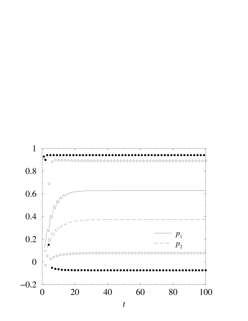
Figure 11: Dynamics of two-cluster synchronization for $a=1.3$, $\epsilon=0.15$ and $N=1000$. The solid circles represent the coordinates of the largest cluster, empty circles those of the second larger cluster, the solid and dashed lines represent their sizes respectively.

A similar route is observed even when the system tends to the completely synchronous period-four orbit. First the system approaches two period-two orbits which are very close one to each other and starts to partition on them. At some point, the smaller cluster is attracted by the larger one and disappears. For some parameter values the period-two orbit remains metastable for quite a long time, until it splits into a period-four orbit through a kind of dynamical bifurcation (see Fig. 12). Even for values of $a$ in the chaotic phase we observed synchronization first through attraction towards prefered period-two orbits and then through a bifurcation (see Fig. 13).

Figure 12: Dynamics of complete synchronization for $a=1.3$, $\epsilon=0.2$ and $N=1000$. Solid circles represent the coordinates of the largest cluster, empty circles (linked by a line to guide the eye) those of the second larger cluster, and the solid line its size $p_{2}$. The second cluster is attracted by the first one and disappears at $t\simeq 40$, but the system continues oscillating on a metastable period-two orbit until, through a dynamical bifurcation, it reaches the stable period-four orbit.

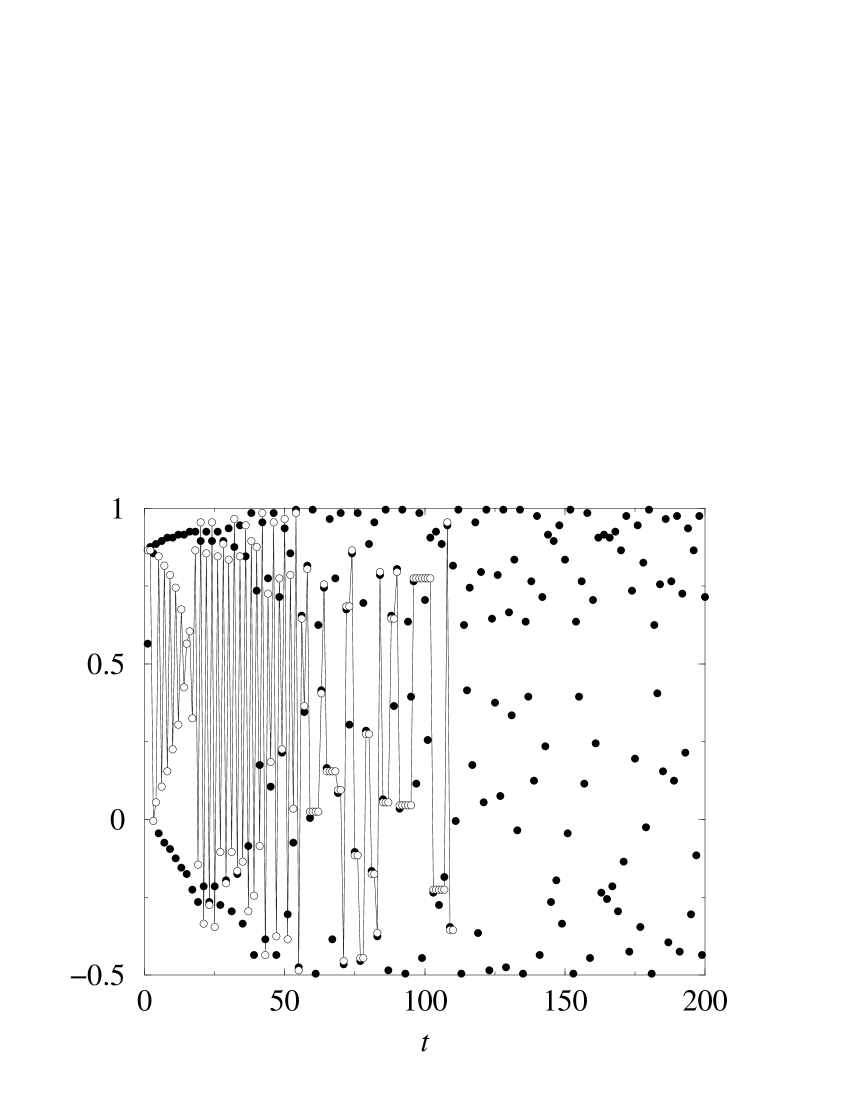
Figure 13: Dynamics of complete synchronization for $a=1.3$, $\epsilon=0.25$ and $N=1000$. Solid circles represent coordinates of the largest cluster, empty circles those of the second larger cluster. The second cluster is attracted by the first one and disappears at $t=110$. The asymptotic dynamics is chaotic, but the largest cluster approaches a metastable period-two orbit in the first stage of the dynamics.

Summaryzing the findings of this section, we can say that the initial synchronization field strongly biases the elements towards a prefered region of phase space, leading them to periodic orbits which can be either stable (and indeed stabilized through the appropriate partition of the system) or metastable (and eventually transformed to completely synchronous attractors).

4.2 Replica-symmetry breakdown in the random-field ensemble

As shown in the previous section, by varying the parameter $\xi$ we can drive the system to macroscopically different attractors. Thus an ensemble of initial conditions, where $\xi$ is randomly chosen for each initial state, is expected to lead to very different attractors. We define a random-field ensemble as a random set of initial conditions which is generated in the following way: For each realization, we first choose at random the parameter $\xi$ form the interval (0,1). Then the initial states $x_{i}(0)$ of all individual maps in the system are independently drawn from the interval $(-\xi,\xi).$

Figure 14: Distributions of overlaps for $a=1.3$ and $\epsilon=0.15$ in the random-field ensemble for different system sizes $N$. The value of $P(1)$ is not represented. It accumulates around 50% of the total weight of $P(q)$.

Figure 15: Distributions of overlaps for $a=1.55$ and $\epsilon=0.1$ in the random-field ensemble for different values of $N$. For these parameters the single map is chaotic. The value of $P(1)\simeq 0$ for all $N$.

When such random-field ensembles of initial conditions are used, overlap distributions do not shrink to a delta-function peak, but remain continuous in the thermodynamic limit. This is shown in Fig. 14, which displays overlap distributions in the random-field ensemble for $a=1.3$ and $\epsilon=0.15$ and different system sizes. In this case, the weight of the completely synchronized attractor, $Y=P(q=1)$ does not vanish in the glassy phase. We expect that the transition to complete synchronization is in this case second-order like: $Y$ tends continuosly to unity as $\epsilon$ approaches the critical coupling at which only synchronized orbits are stable.

We present also the distributions of overlaps for parameters in the chaotic domain of the single map, $\epsilon=0.1$ and $a=1.55$, and three different values of the system size $N$. There is again a qualitative difference between the fixed-field and the random-field ensemble. While in the former case the function $P(q)$ showed a systematic loss of structure for increasing $N$ (see Fig. 1 in MM2 ), in the latter situation it remains remarkably invariant with the growth of the system size.

Thus, we see that for the random-field ensembles of initial conditions the overlap distribution becomes independent of the system syze in thermodynamic limit $N\rightarrow\infty$ . The asymptotic overlap distribution is formed by a delta-peak at $q=1$ plus a broad, smooth part extending to low values of the overlap $q$. The presence of such continuous distribution is an indication of replica-symmetry breaking. The breakdown of replica symmetry means that, for each orbit of GCLM, one can find orbits of gradually varying degrees of similarity within a large ensemble of orbits generated by randomly chosen initial conditions.

4.3 Ultrametricity

Generally, the ultrametric distance $d(A,B)$ between two elements $A$ and $B$ in a hierarchy is defined as the number of steps one should go up in the hierarchy to find a common ancestor of two elements $A$ and $B$. If any three elements $A,$ $B$ and $C$ belong to a hierarchy, the inequality $d(A,C)\leq\max\{d(A,B),d(B,C)\}$ should hold. As a consequence, the two maximal distances between elements in any triad must always be equal. If overlaps $q^{\alpha\beta}$ between any two replicas $\alpha$ and $\beta$ are uniquely determined by the ultrametric distance $d(\alpha,\beta)$ between the respective states, the overlaps between any three replicas $\alpha,\beta$ and $\gamma$ must satisfy the relationship

$$q^{\alpha\gamma}\geq\min\{q^{\alpha\beta},q^{\alpha\gamma}\}\,,$$ (19)

implying that the two minimal overlaps in any triad of replicas are always equal RMP .

To check the presence of ultrametricity, we have to consider triads of replicas $\alpha$, $\beta$, and $\gamma$ and calculate the three overlaps that can be defined by combining them. If the two minimal overlaps in any triad are always equal, the ultrametricity is present. Formally, this amounts to requiring that the relationship (19) always holds. That condition can be numerically tested by generating triads of replicas and computing the distribution $H(\Delta q)$ over the differences between the two minimal overlaps, $\Delta q\equiv|q^{\alpha\beta}-q^{\alpha\gamma}|$. If $H(\Delta q)\to\delta(\Delta q)$ in the limit $N\to\infty$, then the system is ultrametric.

Figure 16: Distribution $H(\Delta q)$ of distances between the two smaller overlaps our of a triad. In the thermodynamic limit this function has a non-vanishing width. Same parameters as in Fig. 15.

Previously, such calculations have been performed for the fixed-field ensemble MM2 . In this case case the distribution $H(\Delta q)$ approaches a delta-function $\delta(\Delta q)$ in the limit of large system sizes $N$. However, as becomes clear from the analysis of overlap distributions in the present study, this behaviour simply reflects the vanishing diversity of system attractors for the fixed-field ensemble in the thermodynamic limit.

We have now repeated such calculations for the random-field ensemble. Distributions $H(\Delta q)$ of distances between the two smaller overlaps in randomly generated triads of replicas for two different system sizes are shown in Fig. 16. We see that the distributions are broad and almost do not depend on the system size. Thus, GCLM do not display ultrametric properties.

Though replica-symmetry breaking is a necessary condition for nontrivial overlap distributions, it does not imply exact ultrametricity, which is a much more demanding condition. Possible deviations from exact ultrametricity have been discussed for spin glasses RMP . Parisi and Ricci-Tersenghi Parisi99 have shown that exact ultrametricity can only hold under the conditions of stochastic stability (i.e. that each replica is in a certain sense equivalent to the others) and of separability (i.e. that all the mutual information about a pair of equilibrium configurations is already encoded in their overlap). Our numerical analysis of GCLM shows that for the random-field ensemble in the thermodynamical limit this system is characterized by replica-symmetry breaking, but exact ultrametricity is absent. Note that though exact ultrametricity, which would have corresponded to the appearance of delta-function peak at $\Delta q=0$, is not observed, the distributions $H(\Delta q)$ in Fig. 16 have a broad maximum at $\Delta q=0$. This indicates that some weaker form of organization may still be present here.

5 Discussion and conclusions

We have examined asymptotic glass properties of globally coupled logistic maps in the thermodynamic limit for two different random ensembles of initial conditions. In the fixed-field ensemble the initial value of the synchronizing field becomes identical up to variations of order $1/\sqrt{N}$ that vanish in the thermodynamic limit.Therefore, all attractors reached by the system become increasingly similar for $N\rightarrow\infty$. Dynamically, the bias due to the initial field drives the system towards the prefered attractor and then the elements partition in such a way to stabilize the prefered attractor. The overlap distribution tends to a delta-function peak at $q=1$, i.e., even when a diverging number of attractors is present, they are all macroscopically identical. Hence, replica symmetry is recoverd for the fixed-field ensemble in the thermodynamic limit.

We have also found that, in the fixed-field ensemble, the system undergoes a special phase transition when $\epsilon$ overcomes a critical value. For smaller coupling, the system is partitioned into a small number (close to the transition, usually two) of periodic orbits. Though all of the attractors reached for different initial conditions are very similar, their number diverges in the thermodynamic limit, and their average attraction basin weight goes to zero. For couplings larger than the critical one, the system synchronizes completely for nearly all initial conditions in the thermodynamic limit, and the average attraction basin weight tends to unity. This situation is reminiscent to the analogous transition in attraction basin weights observed for random boolean networks Bast1 and for asymmetric neural networks Bast2 . In both cases, the average attraction basin goes discountinuously (in the thermodynamic limit) from the value zero, when the system is in the “ordered phase”, to a finite value related to the average attraction basin of random maps REM in the chaotic phase. Though in GCLM the finite attraction basin weight is a consequence of complete synchronization, the formal analogy between this system and dynamical systems with quenched disorder is very suggestive.

The asymptotic behaviour of GCLM in the thermodynamic limit is essentially different when the random-field ensemble of initial conditions is chosen. Because initial synchronizing fields retain in this case macroscopic fluctuations even for $N\rightarrow\infty$, a broad range of attractors may still be reached. In the random-field ensemble, the transition to complete synchronization (with the average attraction basin weight $Y=1$) is expected to be continuous, more in analogy with equilibrium mean-field spin glasses. Examination of the overlap distributions has revealed that replica-symmetry breaking persists in the thermodynamic limit. Thus, GCLM reach the status of a dynamical countepart to mean-field spin glasses.

References

- (1) K. Kaneko, Physica D 41, (1990) 137-172.
- (2) K. Kaneko, Phys. Rev. Lett. 63, (1989) 219-223.
- (3) K. Kaneko and I. Tsuda, Complex systems: Chaos and Beyond (Springer-Verlag, Berlin Heidelberg 2001).
- (4) S.C. Manrubia and A.S. Mikhailov, Europhys. Lett. 50 , (2000) 580-586.
- (5) G. Abramson, Europhys. Lett. 52, (2000) 615-619.
- (6) T. Shibata, T. Chawanya, and K. Kaneko, Phys. Rev. Lett. 82, (1999) 4424-4427.
- (7) N.J. Balmforth, A. Jacobson, and A. Provenzale, Chaos 9, (1999) 738-754.
- (8) M. Mézard, G. Parisi, and M.A. Virasoro, Spin-Glasses Theory and Beyond (World Scientific, Singapore 1987).
- (9) K. Kaneko, J. Phys. A 24 (1991) 2107-2119; Physica D 124, (1998) 322-344.
- (10) A. Crisanti, M. Falcioni, and A. Vulpiani, Phys. Rev. Lett. 76, (1996) 612-615.
- (11) K. Kaneko, Physica D 77, (1994) 456-472.
- (12) S.C. Manrubia and A.S. Mikhailov, Europhys. Lett. 53, (2001) 451-457.
- (13) R. Rammal, G. Toulouse, and M.A. Virasoro, Rev. Mod. Phys. 58, (1986) 765-.
- (14) G. Parisi and F. Ricci-Tersenghi, J. Phys. A 33, (2000) 113-.
- (15) K.H. Fischer and J.A. Hertz, Spin Glasses (Cambridge University Press, Cambridge 1991).
- (16) U. Bastolla and G. Parisi, Physica D 115, (1998) 203-218; ibid. 115, (1998) 219-233.
- (17) U. Bastolla and G. Parisi, J. Phys. A: Math. Gen. 30, (1997) 5613-5631; ibid. 31, (1998) 4583-4602.
- (18) B. Derrida and H. Flyvbjerg, J. de Physique 48, (1986) 971-978.