Numerical Confirmation of Late-time $t^{1/2}$ Growth in Three-dimensional Phase Ordering

Abstract

Results for the late-time regime of phase ordering in three dimensions are reported, based on numerical integration of the time-dependent Ginzburg-Landau equation with nonconserved order parameter at zero temperature. For very large systems ($700^{3}$) at late times, $t\geq 150,$ the characteristic length grows as a power law, $R(t)\sim t^{n}$, with the measured $n$ in agreement with the theoretically expected result $n=1/2$ to within statistical errors. In this time regime $R(t)$ is found to be in excellent agreement with the analytical result of Ohta, Jasnow, and Kawasaki [Phys. Rev. Lett. 49, 1223 (1982)]. At early times, good agreement is found between the simulations and the linearized theory with corrections due to the lattice anisotropy.

PACS: 64.60.Cn 81.10.Aj 05.10.Gg

I Introduction

Phase ordering and phase separation of materials, following a rapid change in an intensive variable from a region of the phase diagram where the system is uniform to one in which two or more phases coexist, are among the oldest and most common methods of materials processing. A typical example is the temperature quenching performed by blacksmiths since antiquity, in which hot metal is suddenly cooled by immersion in water. In fact, the metallurgical term “quenching” has become common in the literature on the dynamics of phase transformations. Modern examples of the use of phase ordering as a processing technique include precipitation strengthening in metals [3] and fabrication of glasses [4].

As the domains of different phases evolve and grow after the quench, the dynamic scaling hypothesis states that their behavior over a large range of length scales can be described in terms of a single, time-dependent characteristic length, $R(t)$. For many phase-ordering processes, this characteristic length behaves as a power law for asymptotically late times,

$$R(t)\sim t^{n},$$ (1)

where the growth exponent $n$ depends on the dynamic universality class [5, 6]. The simplest of these universality classes is comprised of systems with only local relaxational dynamics and a nonconserved scalar order parameter, known as “Model A” in the classification scheme of Hohenberg and Halperin [5]. At late times the order parameter takes distinct values in the two phases, which without loss of generality can be taken as $\pm 1$. The two phases are separated by a sharp interface, where the order parameter is near zero, and the local interface velocity is proportional to the local mean curvature, $H({\bf r},t)$. In two dimensions this is simply the inverse of the local radius of curvature, $R({\bf r},t)$, while in three dimensions it is the arithmetic mean, $H({\bf r},t)=\left[1/R_{1}({\bf r},t)+1/R_{2}({\bf r},t)\right]/2$, where $R_{1}$ and $R_{2}$ are the two principal curvatures. The global characteristic length, $R(t)$, can be identified as proportional to the inverse of the average of $|H({\bf r},t)|$ over the whole interface. It thus obeys the asymptotic equation of motion,

$$\dot{R}(t)\sim 1/R(t)\;,$$ (2)

which yields $n=1/2$, independent of the spatial dimension. This result was shown early on by Lifshitz [7], Chan [8], and Allen and Cahn [9], and it is often referred to as Lifschitz-Allen-Cahn dynamics. Physical realizations of this universality class include phase ordering in anisotropic magnets [6], alloys such as Cu₃Au [10] and Fe₃Al [11], liquid crystals [12, 13], and adsorbate systems [14].

Since experimental complications due to other effects, such as strain fields and hydrodynamics, usually cannot be completely excluded, it is desirable to obtain numerical verification in a cleanly defined three-dimensional model system. Even in two dimensions direct numerical verification of the asymptotic $t^{1/2}$ growth through a direct estimate of $R(t)$ is uncommon; examples are Refs. [14, 15, 16, 17]. A more common practice is to show consistency of numerical results with the asymptotic growth, e.g. through Monte-Carlo Renormalization Group techniques [18, 19] or scaling of the correlation function [20] or structure factor [21]. However, to our knowledge only experimental verifications have so far been reported in three dimensions [10, 13]. Until now, numerical verification has been prevented by the very large systems and long simulation times needed to observe the asymptotic scaling over a sufficient time interval to provide accurate measurements of $n$. In this paper we present such unequivocal confirmation of $t^{1/2}$ growth at late times in three-dimensional numerical simulations of very large systems.

The remainder of this paper is organized as follows. In Sec. II we introduce the numerical model and discuss the numerical method used to integrate its time evolution. In Sec. III we discuss the time evolution at early times. In Sec. IV we present the main numerical results of this paper: the growth of the characteristic length at late and intermediate times. A summary and conclusions are presented in Sec. V.

II Model and Numerical Method

A generic model for the nonconserved dynamics of Model A is given by the time-dependent Ginzburg-Landau (TDGL) equation,

$$\frac{\partial\psi({\bf r},t)}{\partial t}=-\frac{\delta{\cal F}[\psi({\bf r},t)]}{\delta\psi({\bf r},t)}+\zeta({\bf r},t)\;,$$ (3)

where the functional derivative corresponds to the deterministic relaxation associated with the free-energy functional ${\cal F}[\psi({\bf r},t)]$, and $\zeta({\bf r},t)$ is a stochastic process that represents thermal fluctuations. For the local part of the free-energy functional we choose the Ginzburg-Landau-Wilson free energy [6]

$${\cal F}[\psi({\bf r},t)]=\int d{\bf r}\Bigg{[}-\frac{1}{2}\psi^{2}({\bf r},t)+\frac{1}{4}\psi^{4}({\bf r},t)+\frac{c}{2}|{\bf\nabla}\psi({\bf r},t)|^{2}\Bigg{]}\;,$$ (4)

which has minima at $\psi=\pm 1$, corresponding to the two degenerate uniform phases. The problem can be cast into this dimensionless form without loss of generality [21, 22]. The nonequilibrium process associated with a system that is quenched to a temperature far below the critical temperature is controlled by a zero-temperature fixed point [6]. Thus, the stochastic part of Eq. (3) can be ignored, and the equation of motion becomes

$$\frac{\partial\psi({\bf r},t)}{\partial t}=\left(1+c\nabla^{2}\right)\psi({\bf r},t)-\psi^{3}({\bf r},t)\;.$$ (5)

The numerical integration of Eq. (5) with $c=3/2$ [23] was performed using a finite-difference approach on cubic lattices with periodic boundary conditions and $100^{3},$ $300^{3},$ $500^{3},$ and $700^{3}$ points. Results for each system size were averaged over $5$ integrations from different initial conditions, except for the $300^{3}$ lattice, for which results were averaged over $10$ runs. The initial condition consisted of a random value of $\psi$ at each lattice point, with values chosen from a uniform distribution on $[-\psi_{0}$,$\psi_{0}]$. Unless otherwise noted, $\psi_{0}$$=$$0.1$ for results presented here. From this initial configuration, the system was integrated using a first-order Euler scheme with $\Delta t$$=$$0.01$. For early times, $t<10$, we also tried $\Delta t$ reduced by a factor of $5$, which changed $R(t)$ by only about $2\%.$ Approximate isotropy was ensured by using a $19$-point discretization of the Laplacian, analogous to the $9$-point discretization commonly used in two dimensions [24, 25].

The computational resources required for this numerical integration are large. The storage required for one array of $700^{3}$ lattice sites is more than $2.5$ Gigabytes, and two such arrays are required by the integration algorithm. Integration of the $700^{3}$ lattice over $1500$ time units took $84$ hours on $15$ four-processor nodes (5040 CPU hours) on an IBM SP3 supercomputer.

III Early-time Behavior

Immediately after the quench, the local order parameter $\psi\left({\bf r},t\right)$ is randomly distributed with values centered around $0.$ The initial response of the system is to form small regions in local equilibrium, dominated by values near $+1$ or $-1.$ This process is essentially completed by $t\approx 10$, as illustrated in Fig. 1, which shows the time evolution of $\sqrt{\langle\psi^{2}({\bf r},t)\rangle}$ for early times. For the initial condition used here $\langle\psi^{2}({\bf r},0)\rangle=\psi_{0}^{2}/3$ immediately after the quench, and it approaches unity at late times as the regions in local equilibrium come to dominate the system.

The initial relaxation away from the uncorrelated random state, towards a state dominated by regions in which the order parameter everywhere has the same sign, is well described by the linearized version of Eq. (5) (corresponding to a Cahn-Hilliard equation for nonconserved order parameter [26, 27]). The Fourier representation of the solution of this linear dynamical equation is

$$\hat{\psi}\left({\bf k},t\right)=\hat{\psi}\left({\bf k},0\right)\exp{\left[\left(1-ck^{2}\right)t\right]}\;,$$ (6)

where $\hat{\psi}\left({\bf k},t\right)$ is the spatial Fourier transform of the order-parameter field. The progress of the phase ordering at early times can be quantified by $\langle\psi^{2}({\bf r},t)\rangle,$ where $\langle\,\rangle$ represents averaging over space. By integrating $\hat{\psi}({\bf k},t)\hat{\psi}(-{\bf k},t)$ over the ${\bf k}$-space region associated with the finite system, the spatial average can be evaluated as

$$\langle\psi^{2}\left({\bf r},t\right)\rangle=\frac{\langle\psi^{2}({\bf r},0)\rangle}{(2\pi)^{d}}\int{\rm d}{\bf k}\exp{\left(2t\left[1-ck^{2}({\bf k})\right]\right)}\;,$$ (7)

where $d$ is the spatial dimension, and the integration limits are $[-\pi,\pi]$ in each Cartesian coordinate. In deriving this result, we used the fact that the uncorrelated initial condition used here gives $\hat{\psi}({\bf k},0)\hat{\psi}(-{\bf k},0)=\langle\psi^{2}({\bf r},0)\rangle$, independent of ${\bf k}$. In Eq. (7) the expression $k^{2}\left({\bf k}\right)$ takes into account the anisotropy of $k^{2}$ that results from the numerical implementation of the Laplacian. When no anisotropy exists, the integral in Eq. (7) can be evaluated analytically to yield

$$\langle\psi^{2}\left({\bf r},t\right)\rangle=\langle\psi^{2}({\bf r},0)\rangle e^{2t}\left[\frac{{\rm erf}{\left(\pi\sqrt{2ct}\right)}}{2\sqrt{2\pi ct}}\right]^{d}\;.$$ (8)

This result is shown as dashed curves in Fig. 1. For the Laplacian used in the simulations presented here, the anisotropy in the squared magnitude of the wave vector is

$$k^{2}\left({\bf k}\right)=4-\frac{4}{3}\left[\cos{k_{x}}\cos^{2}{\frac{k_{y}}{2}}+\cos{k_{y}}\cos^{2}{\frac{k_{z}}{2}}+\cos{k_{z}}\cos^{2}{\frac{k_{x}}{2}}\right]\;.$$ (9)

Using this expression for $k^{2}({\bf k})$, Eq. (7) was evaluated numerically using midpoint integration at $10^{6}$ uniformly distributed points. The results are presented as the solid curves in Fig. 1, where good agreement is seen between the simulations and the linear theory for $t\lesssim 5$. The initial decrease is due to the diffusional decay of high-wavevector modes with $k^{2}({\bf k})>c^{-1}$. During this brief period one can define a microscopic diffusion length which increases with time as $t^{1/2}$ [16]. The subsequent rapid increase is caused by the exponential growth of the modes at smaller wavevectors. Similar time dependence for $\langle\psi^{2}({\bf r},t)\rangle$ has been observed previously in two-dimensional simulations [16]. As $\psi({\bf r},t)$ approaches unity, the neglected cubic term in the TDGL equation becomes important, and the linear approximation breaks down as the order parameter saturates to its degenerate equilibrium values inside the domains.

To quantify the effects of the initial conditions on the early-time behavior, results for one simulation with $\psi_{0}$$=$$1$ on a $300^{3}$ system are also shown in Fig. 1. Even for this large value of $\psi_{0}$, the linear theory works reasonably well at the earliest times.

IV Late and Intermediate Times

The scaling ansatz associated with Eq. (1) is not valid until a clear separation has been achieved between large-scale fluctuations representing domains in which the order parameter takes values near its two degenerate equilibrium values, and microscopic fluctuations of the local order parameter about these values within the domains [11, 28, 29, 30]. While the early-time growth is completed by $t$$\approx$$10,$ the separation of length scales is not complete until a significantly later time, as is now shown.

For the large simulations presented here, it was necessary to use a computationally efficient estimate of the characteristic length $R(t)$. This was done by identifying $R(t)$ as proportional to the inverse of the interfacial area per unit volume [31, 32]. The interface area was measured by counting the number of the nearest-neighbor lattice-site pairs having values of the local order parameter with opposite signs. As a result,

$$R=\left\{2/(3N)\sum_{\langle i,j\rangle}\Theta\left[-\psi({\bf r}_{i})\psi({\bf r}_{j})\right]\right\}^{-1}-1\;.$$ (10)

Here $N$ is the number of lattice sites, the sum is over all nearest-neighbor pairs, and the Heaviside function $\Theta[x]=0$ for $x\leq 0$ and $1$ otherwise. This definition of $R(t)$ approximates the inverse $r$-derivative of the normalized two-point correlation function, $C(r,t)=C(r/R(t))$, in the small-$r$ limit. Details on the derivation of Eq. (10) are given in the Appendix. Direct comparison with the much more computationally intensive $C(r,t)$ for a 315³ system confirms this equality to within 4% for $t\geq 500$. Corrections to $R$, related to unequal volumes of the degenerate phases [31, 32], which become important at very late times, do not affect the results presented here and have been neglected. The measured values of $R$ are shown in Fig. 2 vs time on a log-log scale. The characteristic length clearly does not obey a single power law for all times. It is only at the latest times, $t\gtrsim 150$, that the asymptotic power-law regime is reached. Least-squares fitting of a power law to the $700^{3}$ data gives an exponent $0.511\pm 0.01$ for $150\leq t\leq 1500$. This result is consistent with the expected value $n=1/2$.

A more sensitive test for true power-law behavior can be made by measuring the instantaneous, effective growth exponent as a function of time. Here this is accomplished by estimating the derivative $d\ln{R}/d\ln{t}$ using 3-point central differencing. The results are presented in Fig. 3. During the early-time regime of near-exponential growth of $\sqrt{\langle\psi^{2}({\bf r},t)\rangle}$, the effective exponent for $R(t)$ falls steeply from near unity at very early times to near $0.40$ around $t\approx 10$. For $t\gtrsim 20$ the effective exponent rises again for the systems larger than $100^{3}$. This steady increase of the effective exponent in the intermediate-time regime indicates that here, too, the dynamics are not properly described by a power law. The only system for which the exponent does become constant is the $700^{3}$ lattice for $t\gtrsim 150.$ For these late times the mean exponent is $0.519\pm 0.01.$ The error on all estimates of the exponent reported here is the standard deviation of these data. Given the trends with system size observed in Figs. 2 and 3, finite-size effects are most likely affecting the late-time behavior in the other system sizes considered here.

A final test for $n=1/2$ at late times is presented in Fig. 4, where $R$ is plotted against $\sqrt{t}.$ The straight line is the least-squares fit of the $700^{3}$ data for $t\geq 150$; it has a correlation coefficient of $0.999976$. The effect of system size on the growth shows a clear trend, with progressively smaller systems departing from the common behavior at progressively earlier times.

It is informative to compare the present results for $R(t)$ to the theoretical prediction of Ohta, Jasnow, and Kawasaki (OJK)[33]. Defined such that the slope of the normalized two-point correlation function $C(r,t)$ is $-1/R(t)$ in the small-$r$ limit, the OJK result is

$$R_{\rm OJK}(t)=\frac{\pi}{2}\sqrt{4c\frac{d-1}{d}t}\;.$$ (11)

In Fig. 2, the OJK result appears as the dashed line, and the agreement with the simulation data at late times is excellent. The OJK theory is similarly successful for the two-dimensional analog of the model presented here, where both the agreement between Eqs. (10) and (11) and the resulting scaled form of the structure factor (the Fourier transform of the two-point correlation function) are excellent [21].

An alternative method to obtain the specific interface area in this system, is to consider the quantity $A(t)=1-\sqrt{\langle\psi^{2}({\bf r},t)\rangle}$, which corresponds to the interface area multiplied with an average interface thickness. Once the interface thickness has converged to a time-independent value, $A^{-1}(t)\propto R(t)$ [25]. For times later than approximately $20,$ $A^{-1}$ increases as a power law with $t$, as shown in Fig. 5. Least-squares fits to the simulation data for $150\leq t\leq 1500$ result in estimated exponents of $0.487\pm 0.01,$ $0.480\pm 0.01,$ and $0.512\pm 0.01$ for the $300^{3},$ $500^{3},$ and $700^{3},$ respectively. An average over the same interval of effective exponents for $A^{-1}(t)$, obtained by 3-point differencing in a way analogous to those discussed above for $R(t)$, give an estimate of $0.511\pm 0.01$ for the 700³ system. These 700³ results, in particular, are thus consistent with $n$=1/2.

V Summary and Conclusions

From the numerical data obtained in this study, we find that the time evolution of the three-dimensional Model A system defined by Eq. (5) can be divided into four time regimes. The time regimes and the evolution behavior in each are summarized as follows.

1. For very early times, before the order parameter has saturated to near its two degenerate equilibrium values inside distinct domains, the time evolution is well described by the linearized version of Eq. (5), as seen in Fig. 1. During this stage, and until $t\approx 10$, the effective exponent of $R(t)$ falls steeply from near unity to near 0.45, as seen in Fig. 3.

2. In the intermediate-time regime, for $10\lesssim t\lesssim 150$, both $R(t)$ and $A^{-1}(t)$ as they are defined here become reasonable measures of a characteristic length, and least-squares fits to log-log plots, such as Fig. 2 and Fig. 5, in this time regime yield apparent exponent estimates near 0.45. However, inspection of Fig. 3 shows that the effective exponent is not constant in this regime: for the systems larger than 100³ it increases steadily back towards the vicinity of 0.5. Thus, the growth of the characteristic length in this intermediate-time regime is also clearly not well described by a simple power law.

3. For late times, $t\gtrsim 150$, and for the largest system studied, 700³, the effective exponent for $R(t)$ [and also for $A^{-1}(t)$] levels off to fluctuate near 0.5. A least-squares fit to $R(t)$ (Fig. 2) over a full decade, $150\lesssim t\lesssim 1500$, yields an estimate of $0.511\pm 0.01$, while an average over the effective exponents (Fig. 3) in the same interval yields $0.519\pm 0.01$. The corresponding estimates for $A^{-1}(t)$ are $0.512\pm 0.01$ and $0.511\pm 0.01$, respectively. These estimates are all consistent with the theoretical expectation of $n$=1/2.

4. For some $t>1500$ for the 700³ system, and indeed for much smaller times for the smaller systems, finite-size effects made observation of $t^{1/2}$ growth impossible. In this very-late-time regime, which is pushed out to later times for larger systems, $R(t)$ becomes on the order of the system size, and the order parameter selects one or the other of its two degenerate values. In Fig. 2, and even more clearly in Fig. 4, it can be seen how $R(t)$ for progressively smaller systems deviates from the asymptotic behavior at progressively earlier times.

We emphasize that, although we see four different time regimes in the domain growth, it is only in the late-stage Lifshitz-Allen-Cahn regime ($150\lesssim t\lesssim 1500$ for the 700³ system) that true power-law growth is observed. While naïve least-squares fits to Fig. 2 indeed yield apparent exponents at early and intermediate times, similar to those recently published by Fialkowski et al. [17], those regimes are not properly described by simple power laws. We also observe from our data that, in disagreement with what is claimed in Ref. [17], the $t^{1/2}$ growth in general is observed at times before the final deviation of the average order parameter from zero. This final loss of symmetry is a finite-size effect, and it occurs only in the very-late-time regime.

In conclusion, we have presented the first unequivocal results confirming $t^{1/2}$ domain growth for integration of a three-dimensional numerical instance of Model A, describing phase ordering in a system with nonconserved order parameter. In this late-time regime of $t^{1/2}$ growth we found excellent agreement between the observed characteristic length and the analytic result of Ohta, Jasnow, and Kawasaki [33]. In order to obtain these solid numerical results, very long simulations of very large systems were necessary.

Appendix

In this Appendix we sketch the derivation of Eq. (10) for the characteristic length $R(t)$ in terms of the total number of bonds between positive and negative nearest-neighbor $\psi({\bf r}_{i})$.

In a $d$-dimensional system with infinitely thin, randomly oriented interfaces, the inverse $r$-derivative of the normalized order-parameter correlation function $C(r,t)$ is [31, 32]

$$R(t)=\left(1-\langle\psi\rangle^{2}\right)V/\left(S\gamma_{d}\right)\;,$$ (12)

where $V$ is the total system volume, $S$ is the total interface area, and the geometric factor $\gamma_{d}$ equals four times the ratio of the volume of a ($d$$-$1)-dimensional sphere to the surface area of a $d$-dimensional sphere of the same radius. On a $d$-dimensional hypercubic lattice of unit lattice constant, the number of bonds broken by the surface of a $d$-dimensional sphere of radius $R$ equals $2d$ times the corresponding discrete approximation to the volume of a $(d-1)$-dimensional sphere of the same radius. The interface area per unit volume, $S/V$, is therefore related to the total number of broken bonds, which is given by the sum in Eq. (10) and here called $\Sigma$, as $S/V=2\Sigma/\left(Nd\gamma_{d}\right)$. The relative error in this estimate comes from the discrete approximation to the $(d-1)$-dimensional volume and is $\propto 1/R$.

The order-parameter dependent factor in Eq. (12) is insignificantly different from unity for the times studied here, and it is therefore ignored. Inserting the expression for $S/V$ in terms of $\Sigma/N$ in Eq. (12) and choosing $d$=3 yields the first term in Eq. (10). The subtraction of unity is included to make $R(t)$ vanish for the random initial condition.

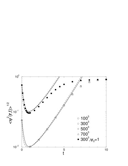
FIG. 1.: Average magnitude of the local order parameter at early times, $\sqrt{\langle\psi^{2}({\bf r},t)\rangle}$, averaged over space and trials, shown vs time on a log-linear scale. The intial decrease at the earliest times is due to diffusional relaxation on short length scales. The near-exponential increase which follows is due to the local relaxation towards one or the other of the degenerate values, $\psi({\bf r},t)\approx\pm 1.$ The solid curves are numerical solutions of the linear theory for the slightly anisotropic Laplacian used here, while the dashed curves correspond to the fully isotropic analytical result, Eq. (8). The solid squares represent a $300^{3}$ simulation with a very wide distribution of initial values, $\psi_{0}=1.$

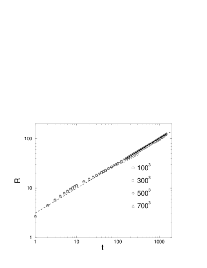
FIG. 2.: The characteristic length $R$ from Eq. (10), shown vs time $t$, on a log-log scale. The dependence of $R(t)$ on the system size indicates that finite-size effects influence the late-time growth exponent. A least-squares fit (the solid line) for the $700^{3}$ system, which should display minimal finite-size effects for the times shown here, yields an exponent estimate of $n$ $=$ $0.511\pm 0.01$ for $t\geq 150.$ The dashed line is the predicted $R(t)$ from Ref. [33], Eq. (11).

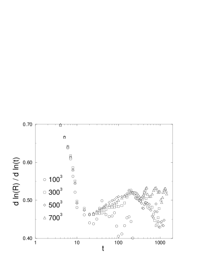
FIG. 3.: Estimate of the instantaneous effective growth exponent vs the central time of the data used for the estimate. See text for details. Simple power-law growth with a constant exponent is seen only for $t>150$ for $700^{3}$, the largest system considered here. Earlier times are clearly not associated with a constant exponent.

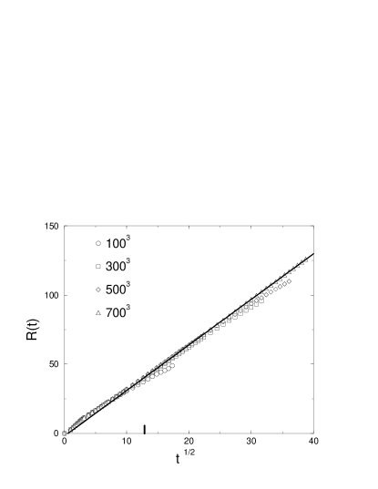
FIG. 4.: A graphical test for $t^{1/2}$ growth in the late-time regime. The onset of finite-size effects occurs at progressively later times as the system size grows. For the $700^{3}$ lattice the finite-size effects are unimportant for the times considered here. The straight line is a least-squares fit to the 700³ data for $t\geq 150$, to the right of the large tick mark.

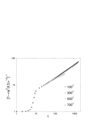
FIG. 5.: The quantity $A^{-1}(t)=\left[1-\sqrt{\langle\psi^{2}({\bf r},t)\rangle}\right]^{-1}$, which at late times is proportional to the characteristic length $R(t)$. The solid line is a least-squares fit to the 700³ data for $t\geq 150$, which yields an estimate for $n$ of $0.512\pm 0.01$.

REFERENCES

- [1] Electronic address: browngrg@csit.fsu.edu
- [2] Electronic address: rikvold@csit.fsu.edu
- [3] H. W. Zandbergen, S. J. Andersen and J. Jansen, Science 277, 1221 (1997).
- [4] M. Tomozawa, in Encyclopedia of Materials Science and Engineering, edited by M. B. Bever (Pergamon, Oxford, 1986), p. 3493.
- [5] P. C. Hohenberg and B. I. Halperin, Rev. Mod. Phys. 49, 435 (1977).
- [6] J. D. Gunton, M. San Miguel and P. S. Sahni, in Phase Transitions and Critical Phenomena, Vol. 8, edited by C. Domb and J. L. Lebowitz (Academic, London, 1983).
- [7] I. M. Lifshitz, Sov. Phys. JETP 15, 939 (1962) [Zh. Éksp. Teor. Fiz. 42, 1354 (1962)].
- [8] S. K. Chan, J. Chem. Phys. 67, 5755 (1977).
- [9] S. M. Allen and J. W. Cahn, Acta Metall. 27, 1085 (1979).
- [10] R. F. Shannon, S. E. Nagler, C. R. Harkless, and R. M. Nicklow, Phys. Rev. B 46, 40 (1992).
- [11] B. Park, G. B. Stephenson, S. M. Allen, and K. F. Ludwig, Phys. Rev. Lett. 68, 1742 (1992).
- [12] N. Mason, A. N. Pargellis, and B. Yurke, Phys. Rev. Lett. 70, 190 (1993).
- [13] I. Dierking, J. Phys. Chem. B 104, 10642 (2000).
- [14] S. J. Mitchell, G. Brown, and P. A. Rikvold, Surf. Sci. 471, 125 (2001).
- [15] O. G. Mouritsen and E. Praestgaard, Phys. Rev. B 38, 2703 (1988).
- [16] F. Corberi, A. Coniglio, and M. Zannetti, Phys. Rev. E 51, 5469 (1995).
- [17] M. Fialkowski, A. Aksimentiev, and R. Holyst, Phys. Rev. Lett. 86, 240 (2001).
- [18] J. Viñals, M. Grant, M. San Miguel, J. D. Gunton, and E. T. Gawlinski, Phys. Rev. Lett. 54, 1264 (1985).
- [19] S. Kumar, J. Viñals, and J. D. Gunton, Phys. Rev. B 34, 1908 (1986).
- [20] A. J. Bray, Adv. Phys. 43, 357 (1994).
- [21] G. Brown, P. A. Rikvold, and M. Grant, Phys. Rev. E 58, 5501 (1998).
- [22] G. Brown, P. A. Rikvold, M. Sutton, and M. Grant, Phys. Rev. E 56, 6601 (1997).
- [23] The coefficient =3/2 was inadvertently introduced through our discretization of the Laplacian. Additional numerical integrations with , performed after this was discovered, did not show any better agreement with the analytic results, nor did they result in a significantly earlier cross-over to the late-time scaling regime. The effect of a value of different from unity is the rescaling of lengths by a factor [21, 22]. This is here taken into account by the inclusion of in Eq. (11).
- [24] Y. Oono and S. Puri, Phys. Rev. Lett. 58, 836 (1987).
- [25] H. Tomita, Prog. Theor. Phys. 85, 47 (1991).
- [26] H. E. Cook, Acta Metall. 18, 297 (1970). Most of the early literature, including this paper, actually considers the linearized equation for conserved order parameter.
- [27] N. A. Gross, W. Klein, and K. Ludwig, Phys. Rev. E 52, 5160 (1997) and references therein.
- [28] C. Billotet and K. Binder, Z. Phys. B 32, 195 (1979).
- [29] G. F. Mazenko, O. T. Valls, and M. Zannetti, Phys. Rev. B 38, 520 (1988).
- [30] B. Morin, K. R. Elder, and M. Grant, Phys. Rev. B 47, 2487 (1993).
- [31] P. Debye, H. R. Anderson, and H. Brumberger, J. Appl. Phys. 28, 679 (1957).
- [32] H. Tomita, in Formation Dynamics and Statistics of Patterns, edited by K. Kawasaki, M. Suzuki, and A. Onuki (World Scientific, Singapore, 1990).
- [33] T. Ohta, D. Jasnow, and K. Kawasaki, Phys. Rev. Lett. 49, 1223 (1982).