Proximity effects at ferromagnet-superconductor interfaces

Abstract

We study proximity effects at ferromagnet superconductor interfaces by self-consistent numerical solution of the Bogoliubov-de Gennes equations for the continuum, without any approximations. Our procedures allow us to study systems with long superconducting coherence lengths. We obtain results for the pair potential, the pair amplitude, and the local density of states. We use these results to extract the relevant proximity lengths. We find that the superconducting correlations in the ferromagnet exhibit a damped oscillatory behavior that is reflected in both the pair amplitude and the local density of states. The characteristic length scale of these oscillations is approximately inversely proportional to the exchange field, and is independent of the superconducting coherence length in the range studied. We find the superconducting coherence length to be nearly independent of the ferromagnetic polarization.

I Introduction

In recent years, technological advances in materials growth and fabrication techniques have made it possible to create heterostructures including high quality ferromagnet/superconductor (F/S) interfaces. These systems have great intrinsic scientific importance and potential device applications, including quantum computers and magnetic information storage[3, 4, 5]. This has led to renewed interest in proximity effects involving magnetic and superconducting compounds. Understanding how proximity effects modify electronic properties near F/S interfaces is constantly becoming more important as the rapid growth of nanofabrication technology continues.

The juxtaposition of a ferromagnet and a superconductor can result[6] in a spatial variation of magnetic and superconducting correlations in both materials. The leakage of superconducting correlations into the non-superconducting material is an example of the superconducting proximity effect. Similarly, the spin polarization may extend into the superconductor and modify its properties, creating a magnetic proximity effect.

In general, if one is interested in a microscopic solution of the F/S proximity effect problem valid at all length scales, one must solve the appropriate equations, e.g. the Gor’kov[7], or Bogoliubov-de Gennes[8] (BdG) equations in a self-consistent manner and with as few approximations as possible. In practice, approximations are often made in the basic equations. Further, in many cases a simple form for the pair potential $\Delta({\bf r})$ is assumed, usually a constant in the superconductor region, and zero elsewhere is used. Such crude non self-consistent treatments have been widely applied because of their simplicity. However they are valid typically only for length scales much longer than the superconducting coherence length, which characterizes the depletion of the pair potential in the superconductor near the interface, or in the case where the non-superconductor is very thin.[9] The superconducting proximity effect is linked to the phenomenon of Andreev reflection[10]. This is the process where at the interface, an electron is reflected as a hole, transmitting a Cooper pair into the superconductor and vice versa. The inhomogeneity in $\Delta({\bf r})$ creates a potential well for quasiparticles, causing electon-hole scattering, and subsequent bound states below the maximum value of $\Delta({\bf r})$.

There are several quantities that can be studied, theoretically or experimentally, in the context of characterizing proximity effects. The traditional description[6] of the superconducting proximity effect is through a characteristic proximity length which can be associated with the behavior of the pair amplitude, $F({\bf r})$, the probability amplitude to find a Cooper pair at point ${\bf r}$. This quantity does not vanish identically inside the non-superconductor. This is in contrast to the pair potential $\Delta({\bf r})$, which is of limited use, since it is zero inside the non-superconducting material unless it is arbitrarily assumed that a small nonvanishing pairing interaction exists there. An additional important quantity, which is now experimentally accessible thanks to improved STM technology[11] which allow local spectroscopy to be performed, is the local density of states (DOS). This quantity reflects the one-particle energy spectrum, and therefore one aspect of the proximity effect.

For a nonmagnetic normal metal in contact with a superconductor, the proximity effect has been much studied and well understood for many years.[6] For clean systems, if the non self-consistent step function for the pair potential is used, solutions to the microscopic equations are relatively easy to obtain.[12, 13, 14, 15] Other approaches involve first simplifying the basic equations. One can, for example, integrate out the energy variable in the Gor’kov equations. The resultant (quasiclassical) Eilenberger[16] equations have the advantage of being first order, and therefore easier to solve. They can be extended to systems of arbitrary impurity concentration.[17] Results that calculate the pair potential self-consistently are more sparse. The Eilenberger equations have been solved numerically, [18] and the DOS was calculated, with comparisons made between self-consistent and non-self-consistent results. For systems in which the electron mean free path is much shorter than the superconducting coherence length, when the Eilenberger equations can be reduced to the simpler Usadel equations[19], a calculation of the DOS[20] has been performed. Numerical approaches which do not require simplifying the starting equations are possible, although rare. Numerical self consistent solutions of the full Gor’kov equations in heterogeneous systems have been obtained,[21, 22] and from these the density of states and pair potential of normal metal-superconductor bilayers and multilayers were calculated.[22]

When the normal metal is replaced by a ferromagnet, the theoretical situation is much less satisfactory. The presence of the exchange field in the ferromagnet makes the overall physical and mathematical picture of the proximity effect in F/S systems quite different from its non-magnetic counterpart. Since on the magnetic side Fermi surface quasiparticles with different spins have different wavevectors, numerical solution becomes much more difficult, as matrices in wavevector space become more complicated, and approximate diagonalization methods such as those employed in Refs. ([21, 22]) cannot be used. The only existing microscopic numerical self-consistent calculations[23, 24] addressing the proximity effect at an F/S interface, are based on an extended Hubbard model in real space. This is adequate only when the coherence length is very short, and the material parameters used[23] were unrealistic. Analytic work is similarly hampered. The traditional[6] way out is to conjecture a dependence of the proximity length on the exchange field, but the underlying assumption, while plausible, has never been proved and has been recently labeled[25] as being just ad hoc. Physically, the spin imbalance in F results in a modified Andreev process, since the electron and hole occupy opposite spin bands.[26] The exchange field causes the quasiparticles comprising a singlet Cooper pair to have different wavevectors, so that the pair amplitude in the ferromagnet becomes spatially modulated.[27] Such oscillations were first investigated long ago by Fulde and Ferrell[28] and Larkin and Ovchinnikov.[29] The resulting oscillations in $F({\bf r})$ induce oscillations (about the normal state value) in the local density of states (DOS) as a function of distance from the interface. These oscillations have been studied theoretically[30] (but non self-consistently) by using the Eilenberger equations, and good agreement was found with experiment.[31] The Usadel equations revealed similar behavior.[32] Quasiclassical approaches are clearly no substitute for a microscopic analysis which is required to study the case when the correlation length is not small.

Thus, the theoretical situation for the F/S interface problem is unsatisfactory. In this paper, we attack this problem by obtaining numerical, fully self-consistent solutions for the continuum BdG equations for a ferromagnet in contact with an $s$-wave superconductor. Our numerical iterative methods overcome the technical difficulties associated with the different Fermi wavevectors, alluded to above, and allow us to focus on the case of longer superconducting coherence lengths in the clean limit. We are able also to allow for different bandwidths in the two materials (Fermi wavevector mismatch[33]). The full BdG equations that are our starting point provide a rigorous, microscopic method for studying inhomogeneous superconductors and their interfacial properties, and have the advantage that their solution provides the quasiparticle amplitudes and excitation energies. The resulting wave functions and energies are used to compute physically relevant quantities. We extract the relevant lengths from analysis of $F(\bf r)$ and investigate the local DOS as a function of position on both sides of the F/S interface. Our results put the entire theory of the F/S proximity effect on firmer grounds, confirm some of the features previously obtained approximately, and uncover new ones.

This paper is organized as follows. In Sec. II, we introduce the spin-dependent BdG equations, and the methods we employ to extract the pair potential, the pair amplitude, and the local DOS. In Sec. III we discuss the physical parameters we will use and present the results. Finally in Sec. IV, we summarize the results and discuss future work.

II Method

In this section we present the basic equations we use for a system containing a ferromagnet/superconductor (F/S) interface and the methods we employ for their self-consistent solution. After self-consistency for the pair potential is achieved, we can then calculate other physically relevant quantities such as the pair condensation amplitude and the local DOS.

The system we consider is semi-infinite and uniform in the $x,y$ directions and confined to the region $0<z<d$, with the F/S interface located at $z=d^{\prime}$ and the superconductor in the region $z>d^{\prime}$. We will take here $d$ and $d^{\prime}$ larger than the other relevant lengths in the problem in order to study the interface between two bulk materials.

We begin with a brief review of the starting equations in order to clarify our notation and conventions, including spin and choice of parameters. For a spatially inhomogeneous system, a complete description of the quasiparticle excitation spectrum along with the quasiparticle amplitudes is given by the BdG equations[8]. In the absence of an applied magnetic field, the system is described, using the usual second quantized form, by an effective mean field Hamiltonian,

$${\cal{H}}_{\rm eff}=\sum_{\sigma,\sigma^{\prime}}{\int{d^{3}r\Bigl{\{}\widehat{\psi}^{\dagger}_{\sigma}({\bf r}){\cal H}_{0}({\bf r})\widehat{\psi}_{\sigma}({\bf r})+\widehat{\psi}^{\dagger}_{\sigma}({\bf r}){h}_{\sigma\sigma^{\prime}}({\bf r})\widehat{\psi}_{\sigma^{\prime}}({\bf r})}}$$ (1)

$$+\frac{1}{2}\eta_{\sigma\sigma^{\prime}}[\Delta({\bf r})\widehat{\psi}^{\dagger}_{\sigma}({\bf r})\widehat{\psi}^{\dagger}_{\sigma^{\prime}}({\bf r})+\Delta^{*}({\bf r})\widehat{\psi}_{\sigma}({\bf r})\widehat{\psi}_{\sigma^{\prime}}({\bf r})]\Bigr{\}},$$ (2)

where $\Delta({\bf r})$ is the pair potential, to be calculated self-consistently, greek indices denote spin, $\widehat{\eta}=i\widehat{\sigma}_{y}$ (the $\widehat{\sigma}$’s are the usual Pauli matrices), and $\widehat{h}({\bf r})=-h_{0}\widehat{\sigma}_{z}\Theta(d^{\prime}-z)$ is the magnetic exchange matrix. The step function in this term reflects the assumption that the exchange field arises from the electronic structure in the F side. The single-particle Hamiltonian is given by,

$${\cal H}_{0}({\bf r})=-\frac{1}{2m}\nabla^{2}+U_{0}({\bf r})-\mu.$$ (3)

Here $\mu$ is the chemical potential, $U_{0}$ is the spin independent mean field term, and we have set $\hbar=k_{B}=1$.

The BdG equations are derived by setting up the diagonalization of the effective Hamiltonian via a Bogoliubov transformation, which in our notation is written as

$$\widehat{\psi}_{\uparrow}({\bf r}) = \sum_{n}{[u_{n\uparrow}({\bf r})\widehat{\gamma}_{n}-{v^{*}_{n\uparrow}({\bf r})\widehat{\gamma}^{\dagger}_{n}]}},$$ (5)

$$\widehat{\psi}_{\downarrow}({\bf r}) = \sum_{n}{[u_{n\downarrow}({\bf r})\widehat{\gamma}_{n}+{v^{*}_{n\downarrow}({\bf r})\widehat{\gamma}^{\dagger}_{n}]}},$$ (6)

where $\widehat{\gamma}$ and $\widehat{\gamma}^{\dagger}$ are Bogoliubov quasiparticle annihilation and creation operators respectively, and $n$ labels the relevant quantum numbers. The quasiparticle amplitudes $u_{n\alpha}$ and $v_{n\alpha}$ are to be determined by requiring that Eqs.(II) diagonalize Eq.(1). The resulting[8] BdG equations read,

$$({\cal H}_{0}+h_{\sigma\sigma})u_{n\sigma}+\sum_{\sigma^{\prime}}{\rho_{\sigma\sigma^{\prime}}\Delta({\bf r})v_{n\sigma^{\prime}}({\bf r})} = \epsilon_{n}u_{n\sigma}({\bf r}),$$ (8)

$$-({\cal H}_{0}+h_{\sigma\sigma})v_{n\sigma}+\sum_{\sigma^{\prime}}{\rho_{\sigma\sigma^{\prime}}\Delta^{*}({\bf r})u_{n\sigma^{\prime}}({\bf r})} = \epsilon_{n}v_{n\sigma}({\bf r}),$$ (10)

where $\widehat{\rho}\equiv\widehat{\sigma}_{x}$, and the $\epsilon_{n}$ are the quasiparticle energy eigenvalues measured with respect to the chemical potential. Equations (II) must be supplemented by the self consistency condition for the pair potential, $\Delta({\bf r})=g({\bf r})\langle\widehat{\psi}_{\uparrow}({\bf r})\widehat{\psi}_{\downarrow}({\bf r})\rangle$, which in terms of the quasiparticle amplitudes reads,

$$\Delta({\bf r})=\frac{g({\bf r})}{2}\sum_{\sigma,\sigma^{\prime}}{\rho_{\sigma\sigma^{\prime}}}{\sum_{n}}^{\prime}{u_{n\sigma}({\bf r})v^{*}_{n\sigma^{\prime}}({\bf r})\tanh(\epsilon_{n}/2T)},$$ (12)

where $g({\bf r})$ is the effective superconducting coupling. We take this quantity to be a constant in the superconductor, and to vanish outside of it. This is analogous to the assumption made for $\widehat{h}$. Our method does not require that a small nonzero value of $g$ be assumed in the non-superconducting side. The prime on the sum in (12) reflects that the sum is only over eigenstates with $|\epsilon_{n}|\leq\omega_{D}$, where $\omega_{D}$ is the cutoff (Debye) energy. The normalization condition for the quasiparticle amplitudes in our geometry is,

$$\sum_{\sigma}\int^{d}_{0}{d^{3}r[|u_{n\sigma}({\bf r})|^{2}+|v_{n\sigma}({\bf r})|^{2}]}=1.$$ (13)

The Hamiltonian is translationally invariant in any plane parallel to the interface, therefore the component of the wavevector perpendicular to the $z$ direction, $k_{\perp}$, is a good quantum number. We can then write

$$u_{n\sigma}({\bf r})=u^{\sigma}_{n}(z)e^{i{\bf k}_{\perp}\cdot{\bf r}},$$ (15)

$$v_{n\sigma}({\bf r})=v^{\sigma}_{n}(z)e^{i{\bf k}_{\perp}\cdot{\bf r}},$$ (16)

where ${\bf k}_{\perp}=(k_{x},k_{y},0)$. Eqs.(II) then become one dimensional BdG equations,

$$\Bigl{[}-\frac{1}{2m}\frac{\partial^{2}}{\partial z^{2}}+\varepsilon_{\perp}+h_{\sigma\sigma}(z)-{\mu}\Bigr{]}u^{\sigma}_{n}(z)$$ (18)

$$+\sum_{\sigma^{\prime}}{\rho_{\sigma\sigma^{\prime}}\Delta(z)v^{{\sigma}}_{n}(z)}=\epsilon_{n}u^{\sigma}_{n}(z),$$ (19)

$$-\Bigl{[}-\frac{1}{2m}\frac{\partial^{2}}{\partial z^{2}}+\varepsilon_{\perp}+h_{\sigma\sigma}(z)-{\mu}\Bigr{]}v^{{\sigma}}_{n}(z)$$ (20)

$$+\sum_{\sigma^{\prime}}{\rho_{\sigma\sigma^{\prime}}\Delta(z)u^{\sigma}_{n}(z)}=\epsilon_{n}v^{{\sigma}}_{n}(z),$$ (21)

where $\varepsilon_{\perp}$ is the transverse kinetic energy, and we have absorbed the mean field term by a shift in the zero of the energies. One can assume $\Delta(z)$ to be real without loss of generality.

We can now solve Eq. (II) by expanding the quasiparticle amplitudes in terms of a complete set of functions $\phi_{m}(z)$,

$$u^{\sigma}_{n}(z) = \sum_{m=1}^{N}u^{\sigma}_{nm}\phi_{m}(z),$$ (23)

$$v^{\sigma}_{n}(z) = \sum_{m=1}^{N}v^{\sigma}_{nm}\phi_{m}(z).$$ (24)

A set of functions appropriate for our setup and geometry is that of the normalized free particle wavefunctions of a one-dimensional box,

$$\phi_{m}(z)=\sqrt{\frac{2}{d}}\sin(k_{m}z),\qquad k_{m}=\frac{m\pi}{d}.$$ (25)

If there was only one Fermi wavevector in the problem, the upper limit in the sum, $N$, would be determined by that wavevector and $\omega_{D}$ in the usual way.[21] But since this is not the case some care is required. The appropriate cutoff for this problem is given by

$$N=[(k_{FX}d/\pi)\sqrt{1+\omega_{D}/\mu}],$$ (26)

where $k_{FX}$ is the largest Fermi wavevector in either the S or F side (see below) and the brackets denote the integer value of the expression they enclose. In a similar way, we can also expand the pair potential,

$$\Delta(z)=\sum_{q=1}^{N}\Delta_{q}\phi_{q}(z).$$ (27)

After inserting these expansions into Eqs.(II) and making use of the orthogonality of the chosen basis, we obtain the following equations for the the matrix elements,

$$\Bigl{[}\frac{k^{2}_{q}}{2m}+\varepsilon_{\perp}\Bigr{]}u^{\sigma}_{nq}-\sum_{q^{\prime}}{\Bigl{[}(E_{FM}-h_{\sigma\sigma})F_{qq^{\prime}}+E_{FS}S_{qq^{\prime}}\Bigr{]}u^{\sigma}_{nq^{\prime}}}$$ (29)

$$+\sum_{\sigma^{\prime}}{\sum_{p,p^{\prime}}}{\rho_{\sigma\sigma^{\prime}}\Delta_{p}J_{pp^{\prime}q}\,v^{{\sigma}}_{np^{\prime}}}=\epsilon_{n}u^{\sigma}_{nq}$$ (30)

$$-\Bigl{[}\frac{k^{2}_{q}}{2m}+\varepsilon_{\perp}\Bigr{]}v^{{\sigma}}_{nq}+\sum_{q^{\prime}}{\Bigl{[}(E_{FM}-h_{\sigma\sigma})F_{qq^{\prime}}+E_{FS}S_{qq^{\prime}}\Bigr{]}v^{{\sigma}}_{nq^{\prime}}}$$ (31)

$$+\sum_{\sigma^{\prime}}{\sum_{p,p^{\prime}}}{\rho_{\sigma\sigma^{\prime}}\Delta_{p}J_{pp^{\prime}q}\,u^{\sigma}_{np^{\prime}}}=\epsilon_{n}v^{{\sigma}}_{nq}.$$ (32)

In writing each term in Eq. (27) we have taken care to measure the chemical potential from the same origin (bottom of the same band) as the corresponding energies. Because of the magnetic polarization and possible differences in carrier densities between the ferromagnet and superconductor, there are up to three different Fermi wavevectors involved in the problem, the two corresponding to spin up and and spin down on the F side, and one in the superconductor. On the F side we have introduced $E_{FM}$ through ${k^{2}_{F\uparrow}}/{2m}\equiv E_{F\uparrow}\equiv E_{FM}+h_{0}$, ${k^{2}_{F\downarrow}}/{2m}\equiv E_{F\downarrow}\equiv E_{FM}-h_{0}$. On the S side, we have ${k^{2}_{FS}}/{2m}=E_{FS}$, where $E_{FS}$ is the appropriate bandwidth. It has been shown,[33] that Fermi wavevector mismatch in F/S tunneling junction spectroscopy leads to nontrivial differences in the conductance spectrum. The matrix elements in (27) are given by,

$$F_{qq^{\prime}} = C_{q^{\prime}-q}(d^{\prime})-C_{q^{\prime}+q}(d^{\prime}),$$ (34)

$$S_{qq^{\prime}} = \delta_{qq^{\prime}}-F_{qq^{\prime}},$$ (35)

$$J_{pp^{\prime}q} = -\frac{1}{\sqrt{2d}}\Bigl{[}E_{q+p^{\prime}-p}(d)-E_{q+p^{\prime}-p}(0)+E_{p+p^{\prime}-q}(d)$$ (36)

$$- E_{p+p^{\prime}-q}(0)+E_{p+q-p^{\prime}}(d)-E_{p+q-p^{\prime}}(0)$$ (37)

$$- E_{p+p^{\prime}+q}(d)+E_{p+p^{\prime}+q}(0)\Bigr{]},$$ (38)

where we have defined $C_{m}(z)\equiv\sin(k_{m}z)/(\pi m)$, $E_{m}(z)\equiv\cos(k_{m}z)/(\pi m)$, for $m\neq 0$, and $E_{0}(z)\equiv 1$. The self-consistency condition now reads,

$$\Delta_{q}=\frac{g}{2}\sum_{p,p^{\prime}}{K_{pp^{\prime}q}\sum_{\sigma,\sigma^{\prime}}{{\sum_{n}}^{\prime}{}\rho_{\sigma\sigma^{\prime}}{u^{\sigma}_{np}v^{{\sigma^{\prime}}}_{np^{\prime}}}\tanh(\epsilon_{n}/2T)}},$$ (39)

where the quantum numbers $n$ include $\varepsilon_{\perp}$ and a longitudinal index $m$, the sum being limited by the restriction mentioned below Eq.(12), and we have,

$$K_{pp^{\prime}q} = -\frac{1}{\sqrt{2d}}\Bigl{[}E_{q+p^{\prime}-p}(d)-E_{q+p^{\prime}-p}(d^{\prime})+E_{p+p^{\prime}-q}(d)$$ (40)

$$- E_{p+p^{\prime}-q}(d^{\prime})+E_{p+q-p^{\prime}}(d)-E_{p+q-p^{\prime}}(d^{\prime})$$ (41)

$$- E_{p+p^{\prime}+q}(d)+E_{p+p^{\prime}+q}(d^{\prime})\Bigr{]}.$$ (42)

Finally, the normalization condition, Eq.(13), in terms of the expansion coefficients, is

$$\sum_{\sigma}\sum_{m}[|u^{\sigma}_{nm}|^{2}+|v^{\sigma}_{nm}|^{2}]=1.$$ (43)

It is very difficult to solve Eqs.(27) numerically as they stand, for large sizes. The required effort can be considerably reduced by solving for $u_{nq}^{\uparrow},v_{nq}^{\downarrow}$ only, allowing for both positive and negative energies. The solutions for $u_{nq}^{\downarrow},v_{nq}^{\uparrow}$ are then obtained via the transformation: $u_{nq}^{\uparrow}\rightarrow v_{nq}^{\uparrow},v_{nq}^{\downarrow}\rightarrow-u_{nq}^{\downarrow},\epsilon_{n}\rightarrow-\epsilon_{n}.$ This simplification follows from the form of the exchange matrix, below Eq.(1). Formally, the exchange field breaks the rotational invariance in spin space,[34] however, there are no spin flip effects, so that the four equations (27) split into two equivalent sets of equations.

For any fixed $\varepsilon_{\perp}$ we can now cast Eqs. (27) as a $2N\times 2N$ matrix eigenvalue problem,

$$\left[\begin{array}[]{cc}H^{+}&D\\ \\ D&H^{-}\end{array}\right]\Psi_{n}=\epsilon_{n}\,\Psi_{n},$$ (47)

where $\Psi_{n}$ is the column vector corresponding to $\Psi_{n}^{T}=(u^{\uparrow}_{n1},\ldots,u^{\uparrow}_{nN},v^{\downarrow}_{n1},\ldots,v^{\downarrow}_{nN}).$ The matrix elements are

$$H^{+}_{qq^{\prime}} = [\frac{k^{2}_{q}}{2m}+\varepsilon_{\perp}]\delta_{qq^{\prime}}-E_{F\uparrow}F_{qq^{\prime}}-E_{FS}S_{qq^{\prime}},$$ (49)

$$H^{-}_{qq^{\prime}} = -[\frac{k^{2}_{q}}{2m}+\varepsilon_{\perp}]\delta_{qq^{\prime}}+E_{F\downarrow}F_{qq^{\prime}}+E_{FS}S_{qq^{\prime}},$$ (50)

$$D_{qq^{\prime}} = \sum_{p}{\Delta_{p}J_{pqq^{\prime}}}.$$ (51)

The basic method of self consistent solution of Eqs. (47) and (39) works as follows: we first choose an initial trial form for the $\Delta_{p}$. We then find, by numerical diagonalization, all the eigenvectors and eigenvalues of the matrix in Eq.(47), for every value of $\varepsilon_{\perp}$ consistent with the energy cutoff (see Eq. (26)). The formally continuous variable $\varepsilon_{\perp}$ is discretized for numerical purposes. The calculated eigenvectors and eigenvalues are then summed according to Eq.(39), and a new pair potential is found. This new pair potential is then substituted[35] into the entire set of eigenvalue equations, and a new set of eigenvalues and eigenvectors is obtained, from which in turn a new pair potential is constructed. The whole process is repeated until convergence is obtained, that is, until the maximum relative change in the pair potential between successive iterations is sufficiently small (see below). As an initial guess for the pair potential one can use, in the first instance, a step function of the bulk value, $\Delta_{0}$, in the superconductor. The initial $\Delta_{p}$ are then obtained by inverting (27). After self-consistent results for $\Delta_{p}$ for one set of parameter values have been obtained, those results can be used as the initial guess for a case involving a nearby set of parameter values. This process reduces the number of required iterations considerably. The final self-consistent result is insensitive to the initial choice. By using these methods, it is then possible, as we shall see, to obtain results even when the coherence length is long.

This general procedure immediately yields the self consistent results for the pair potential. As mentioned in the introduction, this quantity gives valuable information regarding superconducting correlations on the S side ${\it only}$, since it vanishes on the F side where $g({\bf r})=0$. Insight into the superconducting correlations on the F side, and the extraction of the proximity effect in the ferromagnet, is most easily obtained by considering [6, 36] the pair amplitude,

$$F({\bf r})=\Delta({\bf r})/g({\bf r}),$$ (52)

which has a finite value on both sides of the interface. One can also study proximity effects through another quantity which is directly related to observation. This is the local density of states (DOS), given by[37]

$${N}(z,\epsilon)=\sum_{\sigma}{}{\sum_{n}}^{\prime}{[u^{2}_{n\sigma}(z)\delta(\epsilon-\epsilon_{n})+v^{2}_{n\sigma}(z)\delta(\epsilon+\epsilon_{n})]}.\\$$ (53)

In the next section we will first consider the relevant set of dimensionless parameters in the problem, and how we implement the general procedures discussed above for a wide range of the values of these parameters. We then discuss our results, and investigate the length scales relevant to the variation of the pair potential, the pair amplitude and the DOS.

III Results

Before discussing our numerical techniques and results for the model outlined in the previous section, we have to introduce a convenient set of dimensionless parameters for the problem. First, there are two dimensionless ratios arising from the three material parameters $E_{FS}$, $E_{FM}$ and $h_{0}$. We choose the ratio $I\equiv h_{0}/E_{FM}$ as the dimensionless exchange field parameter we will vary to study different degrees of polarization for the F side. $I$ varies between $I$ = 0 when one has a normal (nonmagnetic) metal and $I$ = 1, the half-metallic limit. In this work we choose the second ratio so that $E_{F\uparrow}/E_{FS}$ = 1 at the value of $I$ under consideration. Next, we have to consider the superconducting parameters. We have chosen to present here results for $T=0$, postponing the study of temperature effects for future work. We then need to specify the dimensionless Debye frequency $\omega\equiv\omega_{D}/E_{FS}$ and the dimensionless length scale $k_{FS}\xi_{0}$, where $\xi_{0}$ is the usual zero-temperature coherence length related to other quantities by the BCS relation, $k_{FS}\xi_{0}=(2/\pi)(E_{FS}/\Delta_{0})$. Throughout, we will keep the relatively unimportant parameter $\omega$ fixed at $0.1$, and present results for two different values of $k_{FS}\xi_{0}$, $50$ and $200$. Thus, our method can handle coherence lengths two orders of magnitude larger than what has been achieved through the use[23] of tight binding methods.

We also have to consider the purely computational parameters. These are determined by the overall size of the system, measured in terms of $k_{FS}d$, and the ratio $d^{\prime}/d$. Our two choices of $\xi_{0}$ demand different system sizes, since the length scale over which the pair potential reaches its bulk value in S is determined (see below) by $\xi_{0}$. Thus, we need $d\gg\xi_{0}$ in order to study an interface between bulk systems. Thus, we take $k_{FS}d=1000$, $d^{\prime}/d=600/1000$, for $k_{FS}\xi_{0}=50$, and $k_{FS}d=1700$, $d^{\prime}/d=750/1700$ for $k_{FS}\xi_{0}=200$. These slab widths allow us to investigate fully the bulk proximity effects that occur on both sides of the interface.

The computational work required is chiefly determined by the system size. As outlined in the previous section, we must numerically diagonalize the Hamiltonian matrix and calculate the eigenenergies and eigenvectors for each $\varepsilon_{\perp}$. Each value of $\varepsilon_{\perp}$ requires diagonalizing a matrix of size $2N\times 2N$, where $N$ is defined in Eq. (26). For the large values of $d$ required by our assumed values of $\xi_{0}$ this matrix size exceeds 1100. The number of discretized transverse energies, $N_{\perp}$, must be chosen large enough so that the results are not affected by it. The required value depends on the quantity being studied. For $\Delta(z)$, and $F(z)$, a value of $N_{\perp}=500$ was found to be sufficient even for the longer coherence length. For the local DOS, we used $N_{\perp}=1000$ in both cases. These diagonalizations must be performed at each step in the iteration process described below Eq.(II). The basic diagonalization process employed a procedure whereby the symmetric matrix, Eq.(47), is transformed into tridiagonal form, and then the eigenvalues and eigenvectors are computed by the QL[38] algorithm. The iteration process was concluded when the maximum relative error between successive iterations of the pair potential at any point was less than $10^{-3}$. A smaller relative error would require more computation time, but we verified that no appreciable difference in the results ensued. A number of checks were performed, including reproducing the correct wavefunctions and energies for the limiting case of a single semi-infinite superconductor, ferromagnet or normal metal, and also verifying that in the limit of an entirely superconducting sample the correct finite size oscillations[39, 40] of the pair potential were obtained, with the correct $\xi_{0}$ dependence.[21]

A Pair potential

We begin by presenting in Fig.1 our self consistent results for the pair potential, $\Delta(z)$ (normalized to the bulk value $\Delta_{0}$), which we plot as a function of the dimensionless variable $Z\equiv k_{FS}z$. In the four panels of the left column we show results for $k_{FS}\xi_{0}=50$ for four evenly spaced values of $I$ ranging from zero to unity. In the corresponding panels in the right column we have results

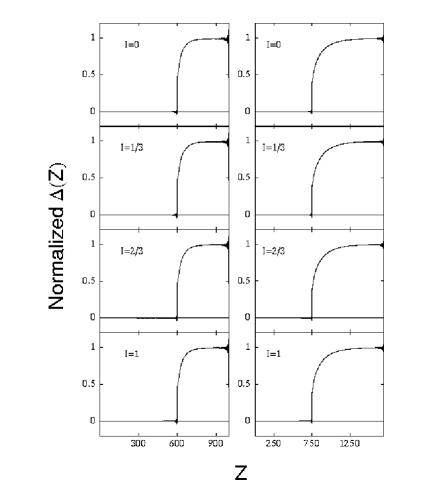
FIG. 1.: The self consistent pair potential $\Delta(z)$, normalized to the bulk value $\Delta_{0}$, is plotted as a function of dimensionless distance $Z\equiv k_{FS}z$. The left column is for $k_{F}\xi_{0}=50$, with the F/S interface at $Z=600$. The right column is for $k_{F}\xi_{0}=200$, the interface is then at $Z=750$. In both cases results for the same four exchange fields (indicated by the labels) are shown.

for $k_{FS}\xi_{0}=200$ at the same values of the exchange field. The pair potential always vanishes on the F side since we assumed $g({\bf r})=0$ in that region. All of the panels show that on the S side, the normalized pair potential rises near the interface and then eventually reaches its bulk value over a length scale determined by the coherence length $\xi_{0}$. Comparing the top panels in each column, where $I=0$, with the others in the figure, where the exchange field can be large, we see that for all four values of $I$ and a given value of $\xi_{0}$, the characteristic depletion near the interface is nearly independent of $I$. It can be concluded therefore, that the magnitude of the exchange field has little effect on $\Delta(z)$ and that the effective coherence length in the superconducting side of the F/S interface is only an extremely weak function of the strength of the ferromagnetic exchange field. Similar findings were obtained in Ref.[23], in the short $\xi_{0}$ limit. The general shape of the curves is the same for both values of $\xi_{0}$, indicating that the effect of this quantity is merely a rescaling of the relevant length which governs the interface depletion. Near the surface-vacuum boundary in S, the pair potential exhibits atomic scale (a distance of order $1/k_{FS}$) oscillations as seen in previous work[21], as a result of pair-breaking by the surface.

B Pair amplitude

The above study of $\Delta(z)$ illustrates the detail, and quality of the results. However, since $\Delta(z)$ vanishes in the F side, this quantity cannot be used to study superconducting proximity effects in the magnet. For this purpose we now turn our attention to the pair amplitude $F(z)$, a quantity that directly reflects[6] the superconducting correlations in both F and S. The main panels in Figure 2, which repeat the arrangement of Fig. 1, show eight sets of results for $F(z)$, four for each of our two values of $k_{FS}\xi_{0}$, for the same values of $I$ as in Fig.1.

FIG. 2.: The pair amplitude $F(z)$ (defined in Eq.(52)), normalized to its bulk value in the superconductor, plotted as a function of dimensionless distance $Z\equiv k_{FS}z$. Results are for the same coherence lengths and exchange fields as in Fig.1, and with the same panel arrangements.

We have normalized $F(z)$ to its bulk value in the superconductor. In the S region the curves are the same as those for the corresponding $\Delta(z)$, seen above in Fig. 1.

Turning our attention to the F side of the interface ($z<d^{\prime}$) in Fig.2, we first look at the normal metal limit ($I=0$) in the top panels. We see that as expected[6, 40] $F(z)$ decays only extremely slowly in the normal region at $T=0$. In effect, there is no mechanism to disrupt the Cooper pairs from drifting across the interface[40], therefore the decay is very slow and occurs over a length scale that is much larger than $\xi_{0}$. The most rapid change occurs near the interface, where $F(z)$ decays very quickly before flattening out.

In the remaining panels of Fig.2 the effects of a finite exchange field are seen. The situation is now very different and $F(z)$ decays to zero rather quickly close to the interface, with a slope that increases with larger $I$. We will see below that the length that characterizes this fast decay varies approximately as $1/I$. This $1/I$ behavior was suggested long ago[6] on the intuitive grounds that the exchange potentials seen by up and down spin quasiparticles differ by $\pm I$, but this argument has been criticized[25] as being merely an ad hoc assumption. Our results show that the intuitive assumption gives the correct result. However, this fast decay is far from the whole story, as slightly away from the interface a much slower oscillatory behavior can be seen (note in particular the $I=1/3$ panel). This is not a finite size effect. We have replotted this behavior in an expanded horizontal scale in Fig.3.

FIG. 3.: Detail of the behavior of the normalized pair amplitude $F(z)$ near the interface, on the magnetic side. The six panels shown correspond to the lower six panels of Fig. 2, but the horizontal scale is expanded so that the oscillatory behavior can be seen.

The wavelength of these oscillations clearly decreases with increased $I$. Furthermore, the magnitude of $F(z)$ also attenuates with increasing $I$. This is in qualitative agreement with past works employing tight-binding[23] or quasiclassical[27] methods.

Before we consider this behavior in more detail let us examine the $\xi_{0}$ dependence of these results for $F(z)$, by comparing the right and left column of Fig. 2. The spatial extent in which the changes in $F(z)$ take place is greater in the right column, since we are dealing now with a length scale given by a longer $\xi_{0}$. Apart from that, the differences are hardly discernible, the only exception being the very slow decay for $I=0$, where the difference can be attributed to the smaller value of $d^{\prime}/\xi_{0}\approx 4$ compared with $d^{\prime}/\xi_{0}\approx 12$ for the case of $k_{FS}\xi_{0}=50$. Thus we conclude that the role of $\xi_{0}$ is, in this range, that of setting an overall scale. This should hold only when $\xi_{0}$ is much larger than the microscopic lengths in the problem and smaller than the geometrical dimensions. It should break down in any other case. The exchange field tends to disrupt superconducting correlations over a length scale that is typically much smaller than $\xi_{0}$, so that the oscillations and characteristic decay of $F(z)$ in the magnetic region are nearly independent of the $\xi_{0}$ considered here.

We are then led to conclude that when there is an exchange field present, there are two phenomena to consider in describing the spatial variations of $F(z)$ in the ferromagnet. The first is the short distance decay at the interface, to the point at which the pair amplitude first goes to zero. This is the region where $F(z)$ changes most rapidly. This decay can be characterized by a length scale which we will denote by $\xi_{1}$, and define as $\xi_{1}\equiv d^{\prime}-z_{1}$, where $z_{1}$ is the first point inside the magnet where $F(z_{1})=0$. The other important phenomenon is the damped oscillations of $F(z)$ in the region $z<z_{1}$ (Fig. 3). These oscillations cannot be fit to an exponentially damped form. Instead, we find that in all cases a much better fit to our results is afforded by the following expression:

$$F(z)=\alpha\frac{{\sin[(z-d^{\prime})/{\xi_{2}}]}}{(z-d^{\prime})/{\xi_{2}}},$$ (54)

where $\alpha$ is a constant, and the characteristic length $\xi_{2}$, which in principle must be distinguished from $\xi_{1}$, can be extracted from the results. Since the previously defined length, $\xi_{1}$, is small, the expression (54) is valid for most of the ferromagnet region. To illustrate the range of its validity, in Fig.4 we give one example of a fit of the form Eq.(54) to the pair amplitude.

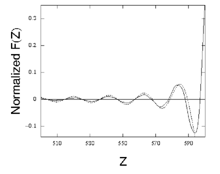
FIG. 4.: Example of a fit of the results for the normalized $F(z)$ (solid curve) to the expression in Eq. (54) (dashed line). The data displayed are for $k_{FS}\xi_{0}=50$ and $I=1/3$ (as shown in Figs. 2 and 3

We see that Eq.(54) is an adequate fit for the oscillatory region, however, within a distance $\xi_{1}$ of the interface, Eq.(54) breaks down. At this point, $F(z)$ rises upwards monotonically to match its value at the interface. In the spatial region where Eq.(54) is valid, the quality of the fits deteriorates somewhat for larger exchange fields ($0.4\lesssim I<1$) because the spatial modulation of $F(z)$ slightly deviates from the simple periodic sine curve given by Eq.(54). This small discrepancy can be glimpsed in the lower panels of Fig.3. The spatial structure becomes slightly nonperiodic, but overall the functional form given by Eq.(54) is still satisfactory.

The oscillatory behavior of the pair amplitude as given by (54) is physically the result[27] of the exchange field, which creates electron and hole excitations in opposite spin bands. The pair amplitude involves products of these particle and hole quasiparticle amplitudes (see Eq.(12)). The superposition of these wavefunctions then creates oscillations on a length scale set by the difference between the spin up and spin down wavevectors in the ferromagnet. One then expects[27] a decay of the form (54) with $\xi_{2}\approx(k_{F\uparrow}-k_{F\downarrow})^{-1}$. We can then write:

$$\xi_{2} \approx \left[\sqrt{2m(E_{FM}+h_{0})}-\sqrt{2m(E_{FM}-h_{0})}\right]^{-1}$$ (55)

$$= k_{FS}^{-1}\frac{\sqrt{1+I}}{\sqrt{1+I}-\sqrt{1-I}},$$ (56)

where in the last step we have used, as previously mentioned, $E_{F\uparrow}/E_{FS}=1$. For small $I$, Eq.(55) can be simplified to $k_{FS}\xi_{2}\approx 1/I$, showing that $\xi_{2}$ is then inversely proportional to the exchange field. At larger values of $I$ there are deviations, but these are small since in the $I=1$ limit both Eq. (56) and the approximate expression coincide. These oscillations are also related to those responsible for oscillatory coupling in structures involving magnetic layers and superconducting spacers, [41] and the nonmonotonic behavior in the critical temperature, $T_{c}$, versus the F-layer thickness in S/F/S junctions.[34] In particular, the sign change in the pair amplitude has the same physical origin as the so called “$\pi$ phase” that exists in F/S multilayers,[42, 43] and the nonmonotonic variation of the Josephson current with exchange field.[44]

Having introduced the two length scales $\xi_{1}$ and $\xi_{2}$ characterizing the superconducting proximity effect in the magnetic region, it is useful to compare their magnitude and behavior as functions of $I$. The result of doing this is shown in Fig.5.

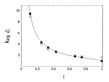
FIG. 5.: Exchange field, $I$, dependence of the lengths $\xi_{i},i=1,2$, defined in the text. The circles are $\xi_{1}$, and the squares represent $\xi_{2}$. The curve is the expression in Eq.(56). The results plotted are for $k_{FS}\xi_{0}=50$ but these quantities are nearly independent of $\xi_{0}$.

Data at additional values of $I$, not displayed in previous Figures, is included. For comparison, Eq.(55) is shown as the solid curve. We find that $\xi_{2}$ follows very closely the expected theoretical expression, and that the other length, $\xi_{1}(I)\approx\xi_{2}(I)$. This is because, as mentioned above, the expression[6] $k_{FS}\xi_{1}=1/I$ nearly coincides numerically with the more complicated result for $\xi_{2}$ as given above. Thus it turns out that the fast decay and the spatial period of the oscillations are characterized by lengths that are virtually identical.

C Local density of states

To further investigate the F/S proximity effects, we focus now on another experimentally accessible quantity, the local DOS. Advances in STM technology[11] have made it possible to perform localized spectroscopic measurements with atomic scale resolution. We therefore present now the local DOS as a function of energy and position, as calculated from Eq.(53) and the self-consistent spectra. All results below are normalized to the normal-state DOS in the S side and convolved with a Gaussian of width $0.01\Delta_{0}$, to eliminate the spectrum discretization resulting from the finite size of the computational sample. We focus only on results for positive energies, since those for negative ones can be obtained by symmetry. We plot the results in terms of the normalized energy variable $\varepsilon/\Delta_{0}$. The locations chosen are given by the dimensionless position measured relative to the interface in terms of the quantity $Z^{\prime}\equiv k_{FS}(z-d^{\prime})$. Thus, a positive value of $Z^{\prime}$ denotes a location within the superconductor.

We consider first the limit where the exchange field $I$ is zero. In Fig.6, we show the DOS for four different positions at each of the two values $k_{FS}\xi_{0}=50$ (left column) and $k_{FS}\xi_{0}=200$ (right column).

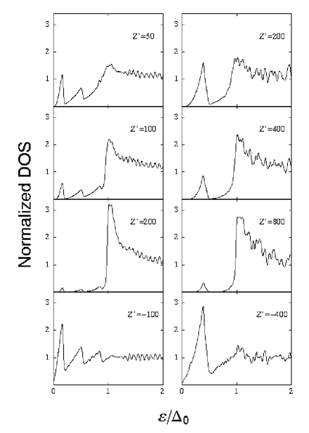
FIG. 6.: Normalized local DOS (see Eq.(53)), plotted versus the dimensionless energy $\varepsilon/\Delta_{0}$ at $I=0$ for $k_{FS}\xi_{0}=50$ (left column) and $k_{FS}\xi_{0}=200$ (right column). The values of the dimensionless quantity $Z^{\prime}\equiv k_{FS}(z-d^{\prime})$ shown by the labels are positions relative to the interface. Each position displayed is a multiple of the coherence length: from top to bottom the rows correspond to $Z^{\prime}=\xi_{0}$, $Z^{\prime}=2\xi_{0}$, $Z^{\prime}=4\xi_{0}$, and $Z^{\prime}=-2\xi_{0}$.

The three top rows in Fig.6 show the DOS on the S side. For the shorter coherence length results for the locations $Z^{\prime}=50,100$, and $200$ are shown. These are multiples of the coherence length, and the same multiples are shown in the right column. Several pronounced peaks are visible inside the gap, due to a finite number of bound states existing for $\varepsilon/\Delta_{0}<1$. These states were predicted long ago in a non self-consistent treatment by de Gennes and Saint-James[13]. These peaks diminish at greater distances inside the superconductor. On the corresponding panels in the right column, we see that the number of de Gennes Saint-James peaks have been reduced. This is because the number of bound states depends upon the coherence length $\xi_{0}$, as well as on the superconductor and normal metal widths[12]. In general, the number of such peaks decreases as $\xi_{0}/d^{\prime}$ increases. The patterns seen at $\varepsilon/\Delta_{0}>1$ are discussed below.

On the normal metal side, we see on the bottom panels of Fig.6, that there is no evidence of a gap, but a pattern of jagged peaks appears in the DOS for $\varepsilon/\Delta_{0}\lesssim 1$. At larger energies, interference patterns are seen, similar to those in the S side. At longer coherence lengths this pattern is more coarse. This coarseness (which is also seen in subsequent figures) arises from the finite value of $N_{\perp}$. If this quantity is increased, the pattern becomes smoother and more regular, as in the left column. The remaining regular oscillations ultimately vanish as $d$ and $d^{\prime}$ tend to infinity. We have chosen to display only one position in the F side for $I=0$ since the overall behavior is nearly identical for all points in the normal metal. This is in agreement with our observation in connection with the $I=0$ panels in Fig.2, that the pair amplitude has a very slow rate of change.

We now turn to the case of a finite exchange field. Figure 7 shows the DOS for $k_{FS}\xi_{0}=50$ (left column), and $k_{FS}\xi_{0}=200$ (right column) at $I=1/3$ for four positions very near the interface, within the magnetic material.

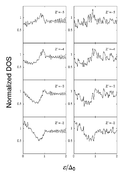
FIG. 7.: Normalized local DOS for $I=1/3$ at four positions in the ferromagnetic side, near the interface. The left column corresponds to $k_{FS}\xi_{0}=50$ and the right one to $k_{FS}\xi_{0}=200$. $Z^{\prime}$ is defined as in the previous Figure.

This is done to illustrate how changes in the local DOS with distance are correlated with the rapid change in $F(z)$ near the interface. Consider first the distance $Z^{\prime}=-5$ (top panels). This corresponds to the location where $F(z)$ has its more prominent minimum (see Fig. 3). There is a weak minimum for the DOS at $\varepsilon/\Delta_{0}=0$, which is more prominent at the smaller $\xi_{0}$, and with increasing energy the DOS rises, until about $\varepsilon/\Delta_{0}\approx 1$ at which point a peak occurs. For energies larger than $\Delta_{0}$ the DOS quickly settles down to its normal state value, unity in our normalization. At $Z^{\prime}=-4$, as $F(z)$ begins to rise, we see, focusing on the range of energies less than $\Delta_{0}$, that the minimum of the DOS has begun to shift away from zero. At $Z^{\prime}=-3$, in the next row of panels, the DOS has now a marked minimum at finite energies within the gap, at $\varepsilon/\Delta_{0}\approx 0.6$. The next position (last row) in Fig.7 shows a clear minimum of the DOS at energies just below the gap. By comparing the top and bottom rows of Fig.7, we see that (for $\varepsilon/\Delta_{0}\lesssim 1$) what were once dips and peaks in the DOS have now reversed roles. Fig.5 shows that the length characterizing the fast rise of $F(z)$ is $k_{FS}\xi_{1}\approx 3.5$ at $I=1/3$. The DOS starts the reversal process, as the interface is approached, at around $Z^{\prime}\approx-3.5$, as seen in Fig. 7. The similarity between right and left columns in this Figure reflects that the length scale $\xi_{1}$, defining the inversion point, is the same in both cases. The behavior of the DOS at larger values of $|Z^{\prime}|$ is qualitatively similar, but as the oscillations die down it becomes much less discernible.

We show also (see Fig.8) the local DOS for three different positions in the superconductor side for the same $I=1/3$ and the shorter $\xi_{0}$.

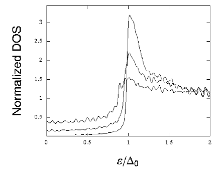
FIG. 8.: Local DOS at three positions inside the superconductor, for $I=1/3$ and $k_{FS}\xi_{0}=50$. The curves shown correspond to (from top to bottom at small energy) $Z^{\prime}=50$, $Z^{\prime}=100$, and $Z^{\prime}=200$. These are the same values as in the top three panels of the left column of Fig. 6.

The de Gennes-Saint James peaks are now gone, with just a hint of small structure for $\varepsilon/\Delta_{0}<1$ remaining at $Z^{\prime}=50$. This structure starts to become washed out at a distance of about $2\xi_{0}$ from the interface. Finally, at $Z^{\prime}=200$, the DOS is of the familiar BCS form, with a well defined gap and pronounced peak at $\varepsilon/\Delta_{0}=1$. In what follows, we focus only on the ferromagnetic region, since the overall behavior of the DOS in S at larger values of $I$ is quite similar to that seen in Fig.8.

In Fig.9, we show the DOS for $I=2/3$.

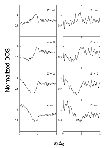
FIG. 9.: Normalized local DOS for $I=2/3$. The panel arrangement is the same as in Fig. 7.

As in Fig.7, we consider four spatial positions for each value of $\xi_{0}$, however the range is now closer to the interface, since the larger exchange field reduces the spatial extent of the superconducting correlations and the length $\xi_{1}$. Beginning at $Z^{\prime}=-4$, Fig.9 (top) illustrates the formation of a small dip at low energies, and a continual rise up to $\varepsilon/\Delta_{0}\approx 1$, after which we recover the bulk DOS limit for a ferromagnet with this polarization. With our normalization, this value is smaller than unity. This is due to the decrease in the number of spin down states with increasing exchange field. In Fig.9 (second row), the minimum in the DOS has moved, while the peak still remains at $\varepsilon/\Delta_{0}\approx 1$. At $Z^{\prime}=-2$, (third row) the DOS is already rising upwards at low energies. The previous dip in the DOS has shifted to a higher energy, while a peak forms around zero energy. We again find consistency with the $\xi_{1}$ values given in Fig.5, where for $I=2/3$, $k_{FS}\xi_{1}\approx 2.2$. Thus, as in the previous case, a reversal of the DOS behavior occurs in the $\xi_{1}$ range. The bottom panel of Fig. 9 shows the DOS at $Z^{\prime}=-1$. We see that the zero energy maximum has increased slightly from the previous row and the minimum has shifted to energy $\Delta_{0}$. Again, this qualitative behavior is independent of $\xi_{0}$ reflecting the independence of $\xi_{1}$ from $\xi_{0}$. Thus, we see here the same behavior we found for $I=1/3$ the only change being the different value of $\xi_{1}$.

We finally consider in Fig.10 the DOS for a fully polarized (half metallic) ferromagnet ($I=1.0$).

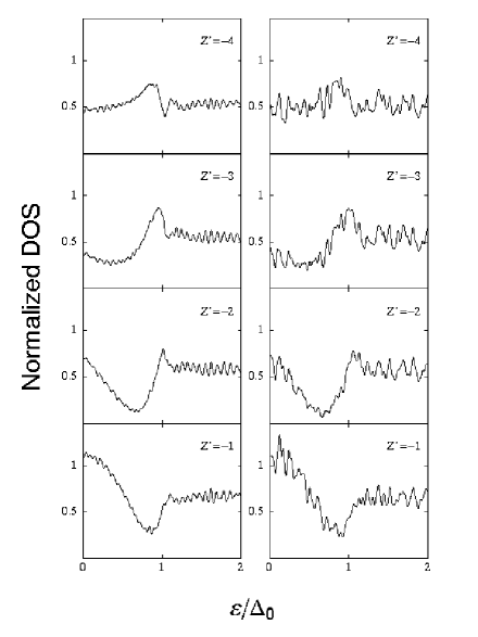
FIG. 10.: Normalized local DOS for a fully polarized ferromagnet ($I=1.0$). Again, results for $k_{FS}\xi_{0}=50$ are in the left column, and those for $k_{FS}\xi_{0}=200$ in the right column, and positions with respect to the interface are indicated.

The locations $Z^{\prime}$ are the same as in Fig.9. The structure of the DOS at energies below the gap for all positions has become smoother. Because of the large exchange field, the reversal of the occupation of states occurs over a length scale $\xi_{1}$ which is now small (see Fig.3). Based on the previous fit in Fig.5, we find this point to be $Z^{\prime}\approx 1.7$. Again, we find consistency between the pair amplitude and the DOS. Note that as one moves away from the interface, the DOS tends to 1/2 at higher energies. This is due to the total absence of the down band in this half metallic limit. These remarks apply to both values of $\xi_{0}$.

The above pertains to the proximity effect in the F side. We now investigate further whether the presence of the ferromagnet has any effect on the superconducting correlations. That any effect is small is shown already by Fig. 2. The influence of the magnet on S will be reflected in a nonzero value of the difference in the density of states for spin-up and spin-down electrons, $\delta N\equiv N_{\uparrow}-N_{\downarrow}$, where $N_{\uparrow}$ and $N_{\downarrow}$ are the spin up and spin down terms in Eq.(53) respectively. One might view this as a self consistent determination of an effective parameter $I(z)$ which may extend into the superconductor. We focus here only on the case of a half metallic ferromagnet ($I=1$), and for illustration take $k_{FS}\xi_{0}=50$. Figure 11 shows that there is in fact a small proximity effect into the superconductor, since very close to the interface the effective polarization is nonzero.

FIG. 11.: Leakage of magnetism into the superconductor: the quantity plotted difference between spin up and spin down values of the local DOS, $\delta N\equiv N_{\uparrow}-N_{\downarrow}$, normalized as in previous Figures. This quantity is displayed at several positions just inside the superconductor. All results shown in this Figure are for $k_{FS}\xi_{0}=50$. The values of $Z^{\prime}$ are indicated in the panels.

This effect is however short ranged, and we see that it nearly dies out before $Z^{\prime}=5$. At very small exchange fields (of order of the superconducting gap), we have found also a longer range proximity effect in the superconductor, similar to that found for dirty systems.[45]

IV conclusions

We have introduced in this paper numerical techniques to accurately and self-consistently solve the continuum BdG equations. We have shown how one can use these methods to perform a detailed study of F/S interfacial properties. Our procedures allow us to consider superconducting and magnetic proximity effects in a bulk system containing an F/S interface, even when the superconducting coherence length is orders of magnitude larger than the interparticle distance. In this work, we have used these techniques to investigate the proximity effects for a clean F/S system. We have extracted the relevant characteristic lengths through a careful analysis of the pair potential and the pair amplitude, and we have shown how, near the interface, the behavior of the pair amplitude correlates with that of the local DOS. Our work extends well beyond previous numerical computations in the tight-binding case, valid only for very short values of $\xi_{0}$, and beyond theoretical work limited by quasiclassical approximations or restricted to regimes where the mean free path or $\xi_{0}$ are very short.

On the S side we have found, near the interface, a depletion of both the pair potential and the pair amplitude. This depletion extends over a length scale determined essentially by $\xi_{0}$, and hence nearly independent of the exchange field $I$. For the bulk heterostructures we considered, the effect of varying $\xi_{0}$ in the range studied ($k_{FS}\xi_{0}=50$ to $k_{FS}\xi_{0}=200$) was an effective rescaling of the characteristic length that determines this depletion. In the F region, for finite values of the exchange field, the pair amplitude exhibited a sharp monotonic decline near the interface, followed by damped oscillations. The fast decay was found to take place over a length scale $\xi_{1}$ approximately inversely proportional to $I$, independent of the $\xi_{0}$, according the the expression[6] $k_{FS}\xi_{1}\approx 1/I$. The oscillatory part of the spatial variation of the pair amplitude could be fit to a simple sine function with an amplitude decaying as the inverse of distance from the interface. We found that the spatial period of the oscillations is determined by the length difference $\xi_{2}=(k_{F\uparrow}-k_{F\downarrow})^{-1}$ (the inverse of the difference between spin up and spin down Fermi wavevectors) provided that $I$ is not too large. This is in reasonable agreement with previous theoretical expectations[27]. We have presented extensive results for the local DOS, as a function of position and energy, as obtained via the self-consistent quasiparticle amplitudes and energies. The periodic sign change in the pair amplitude is found to be correlated with oscillations in the local DOS relative to its normal state values. Finally, we verified also from the local DOS that the effect of the exchange field on superconducting correlations in S is minimal (although nonzero): the difference in the local DOS of spin up and spin down quasiparticles vanishes except very close to the interface, at least for $I\geq 1/3$.

Clearly, the powerful methods and techniques for the self-consistent solution of the BdG equations presented here open new vistas and possibilities for use in the study of many other aspects of the F/S interface and similar problems. A thorough investigation of the physical quantities and characteristic lengths studied in this paper, incorporating other parameter regimes and the effects of finite temperature is needed, and it can be straightforwardly carried out. Interface scattering, and superconductors with nodes in the pair potential (unconventional pair potentials), can be also easily considered. Spin-flip effects, and disorder in both F and S materials can also be incorporated. By suitably changing the boundary conditions, self consistent solutions of the tunneling spectroscopy problem in the long $\xi_{0}$ regime will be obtainable. Our numerical methods are particularly suitable to the study of mesoscopic structures involving F/S multilayers of differing thickness, where size effects may come into play. The study of tunneling phenomena in non-equilibrium situations is also feasible by extension of our method to the time-dependent BdG equations.

- [1] Electronic address: khalter@physics.umn.edu
- [2] Electronic address: otvalls@tc.umn.edu
- [3] G. Blatter, V.B. Geshkenbein, and L.B. Ioffe, Phys. Rev. B63, 174511 (2001)
- [4] S. Oh, D. Youm, and M.R. Beasley, Appl. Phys. Lett. 16, 2376 (1997)
- [5] L.R. Tagirov, Phys. Rev. Lett.83, 2058 (1999)
- [6] G. Deutscher and P.G. de Gennes, in Superconductivity, edited by R.D. Parks (Marcel Dekker, New York, 1969), p. 1005.
- [7] A.L. Fetter and J.D. Walecka, Quantum Theory of Many Particle Systems (McGraw-Hill, New York, 1971).
- [8] P.G. de Gennes, Superconductivity of Metals and Alloys (Addison-Wesley, Reading, MA, 1989).
- [9] G.B. Arnold, Phys. Rev. B18, 1076 (1978)
- [10] A.F. Andreev, Zh. Eksp. Teor. Fiz. 46, 1823 (1964) [Sov. Phys. JETP 19, 1228 (1964)].
- [11] N. Moussy, H Courtois, and B. Pannetier, Rev. Sci. Instrum.,72, 128 (2001).
- [12] M.P. Zaitlin, Phys. Rev. B25, 5729 (1982).
- [13] P.G. de Gennes and D. St.-James, Phys. Lett. 4, 151 (1963).
- [14] W.L. McMillan, Phys. Rev. B175, 559 (1968).
- [15] O. Entin-Wohlman and T. Bar-Sagi, Phys. Rev. B18, 3174 (1978).
- [16] G. Eilenberger, Z. Phys. 214, 195 (1968).
- [17] S. Pilgram, W. Belzig, and C. Bruder, Phys. Rev. B62, 12462 (2000).
- [18] G. Kieselmann, Phys. Rev. B35, 6762 (1987).
- [19] K.D. Usadel, Phys. Rev. Lett.25, 507 (1970).
- [20] W. Belzig, C. Bruder, and G. Schön, Phys. Rev. B54, 9443 (1996).
- [21] B.P. Stojković, and O.T. Valls, Phys. Rev. B47, 5922 (1993).
- [22] B.P. Stojković, and O.T. Valls, Phys. Rev. B50, 3374 (1994).
- [23] J-X Zhu and C.S. Ting, Phys. Rev. B61, 1456 (2000).
- [24] K. Kuboki, Journal Phys. Soc. Japan 68, 3150 (1999).
- [25] M.D. Lawrence and N. Giordano J. Phys. Cond. Matt. 11 1089 (1998).
- [26] M.J.M de Jong, and C.W.J. Beenakker, Phys. Rev. Lett.9, 1657 (1995).
- [27] E.A. Demler, G.B. Arnold, and M.R. Beasley, Phys. Rev. B55,15 174 (1997).
- [28] P. Fulde and A. Ferrell, Phys. Rev. 135, A550 (1964).
- [29] A. Larkin and Y. Ovchinnikov, Sov. Phys. JETP 20, 762 (1965).
- [30] M. Zareyan, W. Belzig, and Y.V. Nazarov, Phys. Rev. Lett.86,308 (2001).
- [31] T. Kontos, M. Aprili, J. Lesueur, and X. Grison, Phys. Rev. Lett.86,304 (2001).
- [32] A. Buzdin, Phys. Rev. B62,11 377 (2000).
- [33] I. Žutić and O.T. Valls, Phys. Rev. B61, 1555 (2000)
- [34] Z. Radović et al, Phys. Rev. B44, 759 (1991)
- [35] In some cases it is more efficient to modify the result of the previous iteration before using it as the next input.
- [36] P.G. De Gennes, Rev. Mod. Phys. 36, 225 (1964).
- [37] See e.g. F. Gygi and M. Schlüter, Phys. Rev. B41,822 (1990).
- [38] The implementation of the subroutine was that in the IBM Engineering and Scientific Subroutine Library (ESSL).
- [39] C.J. Thompson and J.M. Blatt, Phys. Lett. 5, 6 (1963).
- [40] D.S. Falk, Phys. Rev. 132, 1576 (1963).
- [41] O. Šipr and B.L. Györffy, J. Phys.: Condens. Matter 7,5239 (1995).
- [42] A.V. Andreev, A.I. Buzdin, and R.M. Osgood III, Phys. Rev. B43, 10124 (1991).
- [43] I. Baladié, A. Buzdin, N. Ryzhanova, and A. Vedyayev, Phys. Rev. B63,54518 (2001).
- [44] V. Prokić, A.I. Buzdin, and L. Dobrosavljević-Grujić, Phys. Rev. B59,587 (1999).
- [45] R. Fazio and C. Lucheroni, Europhys. Lett. 45, 707 (1999).