XY frustrated systems: continuous exponents in discontinuous phase transitions.

Abstract

XY frustrated magnets exhibit an unsual critical behavior: they display scaling laws accompanied by nonuniversal critical exponents and a negative anomalous dimension. This suggests that they undergo weak first order phase transitions. We show that all perturbative approaches that have been used to investigate XY frustrated magnets fail to reproduce these features. Using a nonperturbative approach based on the concept of effective average action, we are able to account for this nonuniversal scaling and to describe qualitatively and, to some extent, quantitatively the physics of these systems.

I Introduction

After twenty-five years of intense activity, the physics of XY and Heisenberg frustrated systems is still the subject of a great controversy concerning, in particular, the nature of their phase transitions in three dimensions (see for instance Ref. diep94, for a review). On the one hand, a recent high-order perturbative calculation pelissetto00 ; pelissetto01a predicts in both cases a stable fixed point in three dimensions and, thus, a second order phase transition. On the other hand, a nonperturbative approach, the effective average action method, based on a Wilson-like Exact Renormalization Group (ERG) equation, leads to first order transitions tissier00 . Actually, it turns out that, in the Heisenberg case, these two theoretical approaches are almost equivalent from the experimental viewpoint (see however Ref. tissier02b, ). Indeed, within the ERG approach, the transitions are found to be weakly of first order and characterized by very large correlation lengths and pseudo-scaling associated with pseudo-critical exponents close to the exponents obtained within the perturbative approach. This occurence of pseudo-scaling and quasi-universality has been explained within ERG approaches by the presence a local minimum in the speed of the flow zumbach94 ; tissier00 , related to the presence of a complex fixed point with small imaginary parts, called pseudo-fixed pointzumbach94 .

XY frustrated magnets are rather different from this point of view since their nonperturbative RG flows display neither a fixed point nor a minimum. We show in this article that they nevertheless generically exhibit large correlation lengths at the transition and thus, pseudo-scaling, but now without quasi-universality. More precisely, we show that quantities like correlation length and magnetization behave as powers of the reduced temperature on several decades. A central aspect of our approach is that, although the RG flow displays neither a fixed point nor a minimum, it remains sufficiently slow in a large domain in coupling constant space to produce generically large correlation lengths and scaling behaviors. We argue that our approach allows to account for the striking properties of the XY frustrated magnets like the XY Stacked Triangular Antiferromagnets (STA) such as CsMnBr₃, CsNiCl₃, CsMnI₃, CsCuCl₃, as well as XY helimagnets such as Ho, Dy and Tb, which display scaling at the transition without any evidence of universality. Our conclusions are in marked contrast with those drawn from the perturbative approach of Pelissetto et al.  pelissetto00 ; pelissetto01a which leads to predict a second order phase transition for XY frustrated magnets.

II The STA model and its long distance effective hamiltonian

The prototype of XY frustrated systems is given by the STA model. It consists of spins located on the sites of stacked planar triangular lattices. Its hamiltonian reads:

$$H=\sum_{\langle ij\rangle}J_{ij}\vec{S}_{i}.\vec{S}_{j}$$ (1)

where the $\vec{S}_{i}$ are two-component vectors and the sum runs on all pairs of nearest neighbors. The spins interact antiferromagnetically inside the planes and either ferromagnetically or antiferromagnetically between planes, the nature of this last interaction being irrelevant to the long distance physics. Due to the intra-plane antiferromagnetic interactions the system is geometrically frustrated and the spins exhibit a 120^∘ structure in the ground state (see FIG. 1.a).

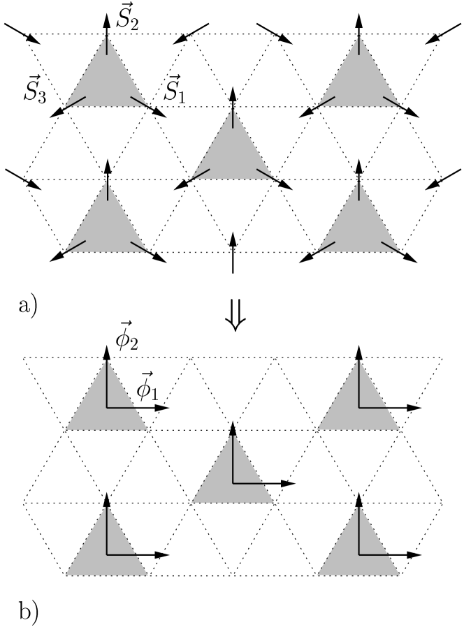
Figure 1: The ground state configurations a) of the spins on the triangular lattice and b) of the order parameter made of two orthonormal vectors. The three-dimensional structure of the ground state is obtained by piling these planar configurations.

As $H$ is invariant under rotation, other ground states can be built by rotating simultaneously all the spins.

Let us describe the symmetry breaking scheme of the STA model in the continuum limit. In the high-temperature phase, the hamiltonian (1) is invariant under the $SO(2)\times{{\mathchoice{\hbox{$\sf\textstyle Z\kern-3.99994ptZ$}}{\hbox{$\sf\textstyle Z\kern-3.99994ptZ$}}{\hbox{$\sf\scriptstyle Z\kern-2.10002ptZ$}}{\hbox{$\sf\scriptscriptstyle Z\kern-0.99998ptZ$}}}}_{2}$ group acting in the spin space and the $O(2)$ group associated to the symmetries of the triangular lattice. In the low-temperature phase, the residual symmetries are given by the group $O(2)_{\hbox{diag}}$ which is a combination of the group acting in spin space and of the lattice group. The symmetry breaking scheme is given byyosefin85 ; kawamura88 :

$$G=O(2)\times SO(2)\times{{\mathchoice{\hbox{$\sf\textstyle Z\kern-3.99994ptZ$}}{\hbox{$\sf\textstyle Z\kern-3.99994ptZ$}}{\hbox{$\sf\scriptstyle Z\kern-2.10002ptZ$}}{\hbox{$\sf\scriptscriptstyle Z\kern-0.99998ptZ$}}}}_{2}\to H=O(2)_{\hbox{diag}}$$ (2)

and thus consists in a fully broken $SO(2)\times{\mathchoice{\hbox{$\sf\textstyle Z\kern-3.99994ptZ$}}{\hbox{$\sf\textstyle Z\kern-3.99994ptZ$}}{\hbox{$\sf\scriptstyle Z\kern-2.10002ptZ$}}{\hbox{$\sf\scriptscriptstyle Z\kern-0.99998ptZ$}}}_{2}$ group. The ${{\mathchoice{\hbox{$\sf\textstyle Z\kern-3.99994ptZ$}}{\hbox{$\sf\textstyle Z\kern-3.99994ptZ$}}{\hbox{$\sf\scriptstyle Z\kern-2.10002ptZ$}}{\hbox{$\sf\scriptscriptstyle Z\kern-0.99998ptZ$}}}}_{2}$ degrees of freedom are known as chirality variables.

Due to the 120^∘ structure, the local magnetization, defined on each elementary plaquette as:

$$\vec{\Sigma}=\vec{S}_{1}+\vec{S}_{2}+\vec{S}_{3}$$ (3)

vanishes in the ground state and cannot constitute the order parameter. In fact, as in the case of colinear antiferromagnets, one has to build the analogue of a staggered magnetization. It is given by a pair of two-component vectors $\vec{\phi}_{1}$ and $\vec{\phi}_{2}$ — defined at the center $\boldsymbol{\sf x}$ of each elementary cell of the triangular lattice — that are orthonormal in the ground state garel76 ; yosefin85 ; kawamura88 (see FIG. 1.b). They can be conveniently gathered into a square matrix:

$$\Phi(\boldsymbol{\sf x})=(\vec{\phi}_{1}(\boldsymbol{\sf x}),\vec{\phi}_{2}(\boldsymbol{\sf x}))\ .$$ (4)

Once the model is formulated in terms of the order parameter, the interaction, originally antiferromagnetic, becomes ferromagnetic. It is thus trivial to derive the effective low-energy hamiltonian relevant to the study of the critical physics which writes:

$$H=-{J\over 2}\int d^{d}\boldsymbol{\sf x}\,\hbox{Tr}\left(\partial^{\;t}\!\Phi(\boldsymbol{\sf x}).\partial\Phi(\boldsymbol{\sf x})\right)$$ (5)

where ${}^{\;t}\!\Phi$ denotes the transpose of $\Phi$.

It is convenient to consider, in the following, a generalization of the models (1) and (5) to $N$-component spins. The order parameter consists in this case in a $N\times 2$ matrix and the symmetry-breaking scheme is thus given by $O(N)\times O(2)\to O(N-2)\times O(2)_{\hbox{diag}}$. Frustrated magnets thus correspond to a symmetry breaking scheme isomorphic to $O(N)\to O(N-2)$ that radically differs from that of the usual vectorial model which is $O(N)\to O(N-1)$. The matrix nature of the order parameter together with the symmetry breaking scheme led naturally in the 70’s to the hypothesis of a new universality class  garel76 ; yosefin85 ; kawamura88 — the “chiral” universality class — gathering all materials supposed to be described by the hamiltonian (1): STA and helimagnets. As we now show, examining the current state of the experimental and numerical data, there is, in fact, no clear indication of universality in the critical behavior of XY frustrated magnets.

III The experimental and numerical context

III.1 The experimental situation

Two kinds of materials are supposed to undergo a phase transition corresponding to the symmetry breaking scheme described above: the STA — CsMnBr₃, CsNiCl₃, CsMnI₃, CsCuCl₃ — (see Ref. perez98, for RbMnBr₃) and the helimagnets: Ho, Dy and Tb. The corresponding critical exponents are given in Table 1.

Note first that, concerning all these data, only one error bar is quoted in the literature, which merges systematic and statistical errors. We start by making the hypothesis that these error bars have a purely statistical origin. Under this assumption, we have computed the — weighted — average values of the exponents and their error bars. This is the meaning of the numbers we give in the following. This hypothesis is however too naïve, and we have checked that, if we attribute a large part of the error bars quoted in Table 1 to systematic bias — typically 0.1 for $\beta$ and 0.2 for $\nu$ —, our conclusions still hold. We also make the standard assumptions that the measured exponents govern the leading scaling behavior, i.e. the determination of the critical exponents is not significantly affected by corrections to scaling. This is generically assumed in magnetic materials where corrections to scaling are never needed to reproduce the theoretical results in the range of reduced temperature reachable in experiments . This is different for fluids where the scaling domain can be very large. Moreover, since the error bars in frustrated systems are much larger than in the usual ferromagnetic systems — by a factor five to ten, see Table 1 — neglecting corrections to scaling should not bias significantly our analysis.

CsMnBr3	$\alpha$=0.39(9), 0.40(5), 0.44(5)
	$\beta$=0.21(1), 0.21(2), 0.22(2), 0.24(2), 0.25(1)
	$\gamma$=1.01(8), 1.10(5); $\nu$=0.54(3), 0.57(3)
CsNiCl3	$\alpha$=0.342(5), 0.37(6), 0.37(8); $\beta$=0.243(5)
CsMnI3	$\alpha$=0.34(6)
CsCuCl3	$\alpha$=0.35(5); $\beta$=0.23(2), 0.24(2), 0.25(2)
Tb	$\alpha$=0.20(3); $\beta$=0.21(2), 0.23(4); $\nu$=0.53
Ho	$\beta$=0.30(10), 0.37(10), 0.39(3),
	0.39(2), 0.39(4), 0.39(4), 0.41(4)
	$\gamma$=1.14(10), 1.24(15); $\nu$=0.54(4), 0.57(4)
Dy	$\beta$=0.38(2), 0.39(1), 0.39${}^{+0.04}_{-0.02}$
	$\gamma$=1.05(7); $\nu$=0.57(5)
STA	$\alpha$= 0.34(6), 0.43(10), 0.46(10)
Monte Carlo	$\beta$= 0.24(2), 0.253(10); $\gamma$=1.03(4), 1.13(5)
	$\nu$=0.48(2), 0.50(1), 0.54(2)
six-loop	$\alpha$=0.29(9); $\beta$=0.31(2); $\gamma$=1.10(4); $\nu$=0.57(3)

Table 1: Critical exponents of the XY frustrated models, from Refs. 2,11-15 and references therein. For CsCuCl₃ the transition has been found of first order and the exponents mentioned here hold only for a reduced temperature larger that 5.10^-3 (see Ref. 16).

Under these assumptions we can analyze the data. We find that there are three striking facts:

i) there are two groups of incompatible exponents. The average value of $\beta$, the best measured exponent, for CsMnBr₃, CsNiCl₃ and Tb — called group 1 — is given by $\beta\sim 0.23$. It is incompatible with that of Ho and Dy — group 2 — which is $\beta\sim 0.39$ (see Table 1 for details). Note that for CsCuCl₃, whose exponents are compatible with those of group 1, the transition has been found to be very weakly of first order weber96 .

ii) the exponents vary much from compound to compound in group 1. For instance, the values of $\alpha$ for CsNiCl₃ and CsMnBr₃ are only marginally compatible.

iii) the anomalous dimension $\eta$ is significantly negative for group 1. For CsMnBr₃, the value of $\eta$ determined by the scaling relation $\eta=2\beta/\nu-1$ with $\beta=0.227(6)$ and $\nu=0.555(21)$ is $\eta=-0.182(38)$. The inclusion of the data coming from CsNiCl₃ and Tb does not change qualitatively this conclusion.

Several conclusions follow from the analysis of the data. From point i), it appears that materials that are supposed to belong to the same universality class differ as for their critical behavior. There are essentially three ways to explain this. In the first one, the two sets of exponents correspond to two true second order phase transitions, each one being described by a fixed point. In the second, one set corresponds to a true second order transition and the other to pseudo-critical exponents associated to weakly first order transitions. In the third, all transitions are weakly of first order.

The first scenario can be ruled out since $\eta$ is negative for group 1 (point iii)) while it cannot be so in a second order phase transition when the underlying field theory is a Ginzburg-Landau $\varphi^{4}$-like theory zinn_eta_pos , as it is the case here yosefin85 . The transition undergone by CsMnBr₃, CsNiCl₃ and Tb is therefore very likely not continuous but weakly of first order. This would explain the lack of universality for the exponents of group 1 (point ii)).

In the second scenario, the materials of group 2 undergo a second order phase transition — $\eta$ is found positive there — while those of group 1 all undergo weakly first order transitions with pseudo-scaling and pseudo-critical exponents. Note that although this scenario cannot be excluded, it is quite unnatural in terms of the usual picture of a second order phase transition. Indeed, it would imply a fine-tuning of the microscopic coupling constants — i.e. of the initial conditions of the flow — for the materials of group 1 in such a way that they lie out of, but very close to, the border of the basin of attraction of the fixed point governing the critical behavior of materials of group 2.

The third scenario, that of generic weak first order behaviors for the two groups of materials, seems even more unnatural, at least in the usual explanation of weak first order phase transitions.

Actually, we shall provide arguments in favor of this last scenario. Also, as we shall see in the framework of the effective average action, the generic character of pseudo-scaling in this scenario has a natural explanation, not relying on the concept of fixed point. Then, no fine-tuning of parameters is required to explain generically weak first order behaviors in frustrated systems.

III.2 The numerical situation

There are no convincing numerical data concerning helimagnets. For the STA system, three different versions have been simulated:

1) the STA itself kawamura92 ; plumer94 ; boubcheur96 .

2) The STAR (Ref. loison98, ) — with R for rigid — which consists in a STA where the fluctuations of the spins around their ground state 120^∘ structure have been frozen. This is realized by imposing the rigidity constraint $\vec{\Sigma}=\vec{S}_{1}+\vec{S}_{2}+\vec{S}_{3}=0$ at all temperatures.

3) A discretized version of the hamiltonian (5), called the Stiefel $V_{2,2}$ model loison98 . There, one considers a system of dihedrals interacting ferromagnetically, which is represented on FIG. 1.b.

At this stage, we emphasize that the rigidity constraint $\vec{\Sigma}=0$ which is imposed in the STAR, as well as the formal manipulations leading to the Stiefel $V_{2,2}$ model affects only the massive — non critical — modes. Thus, all the STA, STAR and Stiefel models have the same critical modes, the same symmetries and thus the same order parameter. One thus could expect a priori that they all exhibit the same critical behavior.

For the STA system, scaling laws are foundkawamura92 ; plumer94 ; boubcheur96 so that a second order behavior could be inferred. The STAR and $V_{2,2}$ models both undergo first order transitionsloison98 . Therefore, by changing microscopic details to go from the STA model to the STAR or $V_{2,2}$ models, the nature of transitions appears to change drastically. This situation indicates that if STA undergoes a genuine second order phase transition, the critical behavior of frustrated magnets in general is characterized by a low degree of universality, a conclusion already drawn from the experimental situation.

With these behaviors one is brought back to the two last scenarios proposed in the previous section: i) the behavior of the STA system is controlled by a fixed point while the STAR and Stiefel models lie outside its basin of attraction ii) all systems undergo first order phase transitions.

In fact, as shown in Ref. loison98, , using the two scaling relations $\eta=2\beta/\nu-1$ and $\eta=2-\gamma/\nu$, $\eta$ is found to be negative in STA systems — although less significantly than in experiments — for all simulations where these calculations can be performed. One can thus suspect a (weak) first order behavior even for the STA system. This hypothesis is strengthened by a recent work of Itakura who has employed Monte Carlo RG techniques in order to investigate the critical behavior of both the STA system and the Stiefel model itakura03 . Using systems with lattice sizes up to $126\times 144\times 126,$ he has provided evidences for weak first order behaviors.

Let us draw first conclusions from the experimental and numerical situations. It appears that the critical physics of frustrated magnets cannot be explained in terms of a single — universal — second order phase transition. A careful analysis of the experimental and numerical data seems to indicate that a whole class of materials undergo (weak) first order phase transitions. At this stage, no conclusion can be drawn about the existence or absence of a true fixed point controlling the physics of some realizations of frustrated magnets. To clarify this issue, we now present the theoretical situation.

IV The theoretical situation

The early RG studies of the STA and helimagnets — and its generalization to $N$-component spins — was performed in a double expansion in coupling constant and in $\epsilon=4-d$ on the Ginzburg-Landau-Wilson (GLW) version of the model in Refs. jones76, ; bak76, ; garel76, ; yosefin85, . It has appeared that, for a given dimension $d$, there exists a critical number of spin component, called $N_{c}(d)$, above which the transition is of second order and below which it is of first order. Naturally, a great theoretical challenge in the study of frustrated magnets, has been the determination of $N_{c}(d)$. Its value has been determined within perturbative computation at three-loop order pelissetto01b :

$$N_{c}(4-\epsilon)=21.8-23.4\epsilon+7.09\epsilon^{2}+O(\epsilon^{3})\ .$$ (6)

Unfortunately, this series is not well behaved since the coefficients are not decreasing fast. It has been conjectured by Pelissetto et al. pelissetto01b that $N_{c}(2)=2$. Using this conjecture, these authors have reexpressed (6) in the form:

$$N_{c}(4-\epsilon)=2+(2-\epsilon)(9.9-6.77\epsilon+0.16\epsilon^{2})+O(\epsilon^{3})\ .$$ (7)

The coefficients of this expression are now rapidly decreasing so that it can be used to estimate $N_{c}(d)$. For $d=3$ it provides $N_{c}(3)=5.3$ and leads to the conclusion that the transition is of first order in the relevant Heisenberg and XY cases.

In agreement with this result, the perturbative approaches performed at three loops, either in $4-\epsilon$ or directly in three dimensions, lead to a first order phase transition for XY systems with a $N_{c}(3)$ given respectively by $N_{c}(3)=3.91$ (Ref. antonenko94, ) and $N_{c}(3)=3.39$ (Ref. antonenko95, ). However, according to the authors, these computations are not well converged. It is only recently that a six-loop calculation has been performed pelissetto00 ; pelissetto01a directly in three dimensions which is claimed to be converged in the Heisenberg and XY cases. Note that, for values of $N$ between $N\simeq 5$ and $N\simeq 7$, the resummation procedures do not lead to converged results, forbidding the authors to compute $N_{c}(3)$ in this way. For $N=2$ and $N=3$ a fixed point is found. The exponents associated to the $N=2$ case are given in Table 1. Note that $\gamma$ and $\nu$ compare reasonably well with the experimental data of group 1. However, as we already stressed, the existence of a fixed point implies $\eta>0$ — $\eta=0.08$ in Ref. pelissetto01a, — and is thus incompatible with the negative value of $\eta$ found for the group 1. Moreover, the value $\beta=0.31(2)$ found in Ref. pelissetto01a, is far — 4 standard deviations — from the average experimental value $\beta=0.237(6)$ for group 1 and also far — 3.7 standard deviations — from that obtained from group 2, Ho and Dy: $\beta=0.388(7)$. It is thus incompatible with the two sets of experimental values. This point strongly suggests that the six-loop fixed point neither describes the physics of materials belonging to group 2 that, in the simplest hypothesis, should also undergo a first order phase transition.

The preceding discussion does not rule out the existence of the fixed point found in Ref. pelissetto01a, . This just shows that, if it exists, it must have a very small basin of attraction, and that the initial conditions corresponding to the STA and helimagnets lie out of it. In fact, as we argue in the following, this fixed point probably does not exist at all so that we expect that all transitions are of (possibly very weak) first order.

V The exact RG approaches

There exists an alternative theoretical approach to the perturbative RG calculations which explains well, qualitatively and to some extent quantitatively, all the preceding facts. It relies on the Wilsonian RG approach to critical phenomena, based on the concept of block spins and scale dependent effective theorieskadanoff66 ; wilson74 . Although it has been originally formulated in terms of hamiltonians, its most recent and successful implementation involves the effective (average) actionwetterich93c ; ellwanger94c ; morris94a . In the same way as in the original Wilsonian approach, one constructs an effective action, noted $\Gamma_{k}$, that only includes high-energy fluctuations — with momenta $q^{2}>k^{2}$ — of the microscopic system. At the lattice scale $k=\Lambda=a^{-1}$, $\Gamma_{k}$ corresponds to the classical Hamiltonian $H$ since no fluctuation has been taken into account. When the running scale $k$ is lowered, $\Gamma_{k}$ includes more and more low-energy fluctuations. Finally, when the running scale is lowered to $k=0$, all fluctuations have been integrated out and one recovers the usual effective action or Gibbs free energy $\Gamma$. To summarize one has:

$$\left\{\begin{array}[]{ll}\Gamma_{k=\Lambda}=H\\ \\ \Gamma_{k=0}=\Gamma\ .\end{array}\right.$$ (8)

Note also that the original hamiltonian depends on the original spins while the effective action — at $k=0$ — is a function of the order parameter. At an intermediate scale $k$, $\Gamma_{k}$ is a function of an average order parameter at scale $k$ noted $\phi_{k}(q)$ — or more simply, $\phi(q)$ — that only includes the fluctuations with momenta $q^{2}>k^{2}$. Thus $\Gamma_{k}$ has the meaning of a free energy at scale $k$.

At a generic intermediate scale $k$, $\Gamma_{k}$ is given as the solution of an exact equation that governs its evolution with the running scale tetradis94 :

$${\frac{\partial\Gamma_{k}[\phi]}{\partial t}}=\frac{1}{2}\hbox{Tr}\left\{\left(\Gamma_{k}^{(2)}[\phi]+R_{k}\right)^{-1}\frac{\partial R_{k}}{\partial t}\right\}\;,$$ (9)

where $t=\ln\displaystyle{(k/\Lambda)}$ and the trace has to be understood as a momentum integral as well as a summation over internal indices. In Eq.(9), $\Gamma_{k}^{(2)}[\phi]$ is the exact field-dependent inverse propagator i.e. the second functional derivative of $\Gamma_{k}$. The quantity $R_{k}$ is the infrared cut-off which suppresses the propagation of modes with momenta $q^{2}<k^{2}$. A convenient cut-off, that realizes the constraints (8), is provided by litim00 :

$$R_{k}(q^{2})=Z(k^{2}-q^{2})\theta(k^{2}-q^{2})$$ (10)

where $Z$ is the $k$-dependent field renormalization.

Ideally, in order to relate the thermodynamical quantitites to the microscopic ones, one should integrate the flow equation starting from $k=\Lambda$ with the microscopic hamiltonian $H$ as an initial condition and decrease $k$ down to zero. However, Eq.(9) is too complicated to be solved exactly and one has to perform approximations. To render Eq.(9) manageable, one truncates the effective action $\Gamma_{k}[\phi]$ to deal with a finite number of coupling constants. The most natural truncation, well suited to the study of the long distance physics of a field theory, is to perform a derivative expansion tetradis94 of $\Gamma_{k}[\phi]$. This consists in writing an ansatz for $\Gamma_{k}$ as a series in powers of $\partial\phi$. The physical motivation for such an expansion is that since the anomalous dimension $\eta$ is small, terms with high numbers of derivatives should not drastically affect the physics.

Actually, another truncation is performed. It consists in expanding the potential, which involves all powers of the $O(N)\times O(2)$ invariants built out of $\vec{\phi}_{1}$ and $\vec{\phi}_{2}$, in powers of the fields. This kind of approximation allows to transform the functional equation (9) into a set of ordinary coupled differential equations for the coefficients of the expansion. It has been shown during the last ten years that low order approximations in the field expansion give very good results (see Ref. berges02, for a review and Ref. bagnuls01, for an exhaustive bibliography). The simplest such truncation is tissier00 :

$$\begin{split}\Gamma_{k}=\int d^{d}x\Bigg{\{}&\frac{Z}{2}\hbox{Tr}\left(\partial^{\;t}\!\Phi.\partial\Phi\right)+\frac{\omega}{4}(\vec{\phi}_{1}.\partial\vec{\phi}_{2}-\vec{\phi}_{2}.\partial\vec{\phi}_{1})^{2}+\\ &+\frac{{\lambda}}{4}\left({\rho\over 2}-{\kappa}\right)^{2}+\frac{{\mu}}{4}\tau\Bigg{\}}\ .\end{split}$$ (11)

Let us first discuss the different quantities involved in this expression. One recalls that $\Phi$ is the $N\times 2$ matrix gathering the $N$-component vectors $\vec{\phi}_{1}$ and $\vec{\phi}_{2}$ (see Eq.(4)). There are two independent $O(N)\times O(2)$ invariants given by $\rho={\hbox{Tr}}\,^{t}\Phi\Phi$ and $\tau=\frac{1}{2}{\hbox{Tr}}\,(^{t}\Phi\Phi)^{2}-\frac{1}{4}({\hbox{Tr}}\ ^{t}\Phi\Phi)^{2}$. The set $\left\{\kappa,\lambda,\mu,Z,\omega\right\}$ denotes the scale-dependent coupling constants which parametrize the model at this order of the truncation. The first quantity in Eq.(11) corresponds to the standard kinetic term while the third and fourth correspond to the potential part. Actually, apart from the second term — called the current term —, $\Gamma_{k}$ in Eq.(11) looks very much like the usual Landau-Ginzburg-Wilson action used to study perturbatively the critical physics of the $O(N)\times O(2)$ model, up to trivial reparametrizations. There is however a fundamental difference since we do not use $\Gamma_{k}$ within a weak-coupling perturbative approach. This allows the presence of the current term which corresponds to a non-standard kinetic term. This term is irrelevant by power counting around four dimensions since it is quartic in the fields and quadratic in derivatives. However its presence is necessary around two dimensions to recover the results of the low-temperature approach of the nonlinear sigma (NL$\sigma$) model since it contributes to the field renormalization of the Goldstone modes. Being not constrained by the usual power counting we include this term in our ansatz. Note also that we have considered much richer truncations than that given by Eq.(11) by putting all the terms up to $\Phi^{10}$ and by adding all terms with four fields and two derivatives. This has allowed us to check the stability of our results with respect to the field expansion.

We do not provide the details of the computation. The general technique is given in several publications and its implementation on the specific $O(N)\times O(2)$ model will be given in a forthcoming articletissier02b . The $\beta$ functions for the different coupling constants entering in (11) are given by:

$$\begin{split}\frac{d\kappa}{dt}=&-(d-2+\eta)\kappa+4v_{d}\bigg{[}\frac{1}{2}l_{01}^{d}(0,0,\kappa\omega)+(N-2)l_{10}^{d}(0,0,0)+\frac{3}{2}l_{10}^{d}(\kappa\lambda,0,0)+\left(1+2\frac{\mu}{\lambda}\right)l_{10}^{d}(\kappa\mu,0,0)+\\ &+\frac{\omega}{\lambda}l_{01}^{2+d}(0,0,\kappa\omega)\bigg{]}\end{split}$$ (12a)

$$\begin{split}\frac{d\lambda}{dt}=&(d-4+2\eta)\lambda+v_{d}\bigg{[}2\lambda^{2}(N-2)l_{20}^{d}(0,0,0)+\lambda^{2}l_{02}^{d}(0,0,\kappa\omega)+9\lambda^{2}l_{20}^{d}(\kappa\lambda,0,0)+2(\lambda+2\mu)^{2}l_{20}^{d}(\kappa\mu,0,0)+\\ &+4\lambda\omega l_{02}^{2+d}(0,0,\kappa\omega)+4\omega^{2}l_{02}^{4+d}(0,0,\kappa\omega)\bigg{]}\end{split}$$ (12b)

$$\begin{split}\frac{d\mu}{dt}=&(d-4+2\eta)\mu-2v_{d}\mu\bigg{[}-\frac{2}{\kappa}l_{01}^{d}(0,0,\kappa\omega)+\frac{3(2\lambda+\mu)}{\kappa(\mu-\lambda)}l_{10}^{d}(\kappa\lambda,0,0)+\frac{8\lambda+\mu}{\kappa(\lambda-\mu)}l_{10}^{d}(\kappa\mu,0,0)+\\ &+\mu l_{11}^{d}(\kappa\mu,0,\kappa\omega)+\mu(N-2)l_{20}^{d}(0,0,0)\bigg{]}\end{split}$$ (12c)

$$\begin{split}\eta=&-\frac{d\;\ln Z}{dt}=2\frac{v_{d}}{d\kappa}\bigg{[}(4-d)\kappa\omega l_{01}^{d}(0,0,\kappa\omega)+2\kappa^{2}\omega^{2}l_{02}^{2+d}(0,0,\kappa\omega)+2m_{02}^{d}(0,0,\kappa\omega)-4m_{11}^{d}(0,0,\kappa\omega)+\\ &+2(-2+d)\kappa\omega l_{10}^{d}(0,0,0)+2m_{20}^{d}(0,0,\kappa\omega)+2\kappa^{2}\lambda^{2}m_{2,2}^{d}(\kappa\lambda,0,0)+4\kappa^{2}\mu^{2}m_{2,2}^{d}(\kappa\mu,0,0)+\\ &+4\kappa\omega n_{02}^{d}(0,0,\kappa\omega)-8\kappa\omega n_{11}^{d}(0,0,\kappa\omega)+4\kappa\omega n_{20}^{d}(0,0,\kappa\omega)\bigg{]}\end{split}$$ (12d)

$$\begin{split}\frac{d\omega}{dt}=&(d-2+2\eta)\omega+\frac{4v_{d}}{d\kappa^{2}}\bigg{[}\kappa\omega\bigg{\{}\frac{(4-d)}{2}l_{01}^{d}(0,0,\kappa\omega)+\frac{(d-16)}{2}l_{01}^{d}(\kappa\lambda,0,\kappa\omega)+\kappa\omega l_{02}^{2+d}(0,0,\kappa\omega)-\\ &-3\kappa\omega l_{02}^{2+d}(\kappa\lambda,0,\kappa\omega)+(d-2)l_{10}^{d}(0,0,0)-(d-8)l_{10}^{d}(\kappa\lambda,0,0)+8\kappa\lambda l_{11}^{d}(\kappa\lambda,0,\kappa\omega)+2\kappa\omega l_{20}^{2+d}(\kappa\mu,0,0)\\ &+2\kappa\omega(N-2)l_{20}^{2+d}(0,0,0)\bigg{\}}+m_{02}^{d}(0,0,\kappa\omega)-m_{02}^{d}(\kappa\lambda,0,\kappa\omega)-2m_{11}^{d}(0,0,\kappa\omega)+2m_{11}^{d}(\kappa\lambda,0,\kappa\omega)+\end{split}$$ (12e)

$$\begin{split}&+m_{20}^{d}(0,0,\kappa\omega)-m_{20}^{d}(\kappa\lambda,0,\kappa\omega)+\kappa^{2}\lambda^{2}m_{22}^{d}(\kappa\lambda,0,0)+2\kappa^{2}\mu^{2}m_{22}^{d}(\kappa\mu,0,0)+2\kappa\omega n_{02}^{d}(0,0,\kappa\omega)-\\ &-4\kappa\omega n_{02}^{d}(\kappa\lambda,0,\kappa\omega)-4\kappa\omega n_{11}^{d}(0,0,\kappa\omega)+8\kappa\omega n_{11}^{d}(\kappa\lambda,0,\kappa\omega)+2\kappa\omega n_{20}^{d}(0,0,\kappa\omega)-4\kappa\omega n_{20}^{d}(\kappa\lambda,0,\kappa\omega)\bigg{]}\end{split}$$

In these equations appear the dimensionless functions $l_{n1,n2}^{d},m_{n1,n2}^{d},n_{n1,n2}^{d}$, called threshold functions, since they govern the decoupling of the massive modes entering in the action (11). They encode the nonperturbative content of the flow equations (12). They are complicated integrals over momenta and are explicitly given in the Appendix.

VI Results and physical discussion

VI.1 Checks of the method

We have first proceeded to all possible checks of our method by comparing our results with all available data obtained within the different pertubative approaches. Our method fulfills all these checks.

1) Around $d=4$, we have checked that, in the limit of small coupling constant, our equations degenerate in those obtained from the weak coupling expansion at one loopjones76 ; bak76 ; garel76 :

$$\left\{\begin{aligned} {d\lambda\over dt}&=(d-4)\lambda+\frac{1}{16\pi^{2}}\left(4\lambda\mu+4\mu^{2}+\lambda^{2}(N+4)\right)\\ {d\mu\over dt}&=(d-4)\mu+\frac{1}{16\pi^{2}}\left(6\lambda\mu+N\mu^{2}\right).\end{aligned}\right.$$ (13)

This can be easily verified considering the asymptotic expressions of the threshold functions that are given in the Appendix.

2) Also, around $d=2$, performing a low-temperature expansion — corresponding to a large $\kappa$ expansion — of our equations and making the change of variables:

$$\left\{\begin{aligned} \eta_{1}&=2\pi\kappa\\ \eta_{2}&=4\pi\kappa(1+\kappa\omega)\\ \end{aligned}\right.$$ (14)

one recovers the $\beta$-functions found in the framework of the nonlinear $\sigma$ model at one loopazaria93 :

$$\left\{\begin{aligned} \beta_{1}&=-(d-2)\eta_{1}+N-2-\frac{\eta_{2}}{2\eta_{1}}\\ \beta_{2}&=-(d-2)\eta_{2}+\frac{N-2}{2}\left(\frac{\eta_{2}}{\eta_{1}}\right)^{2}\ .\ \end{aligned}\right.$$ (15)

This shows that our method allows to recover the perturbative results both near $d=2$ and $d=4$. This is not a surprise since, as well known, Eq.(9) has a one-loop structure. However, for frustrated magnets, and contrary to the $O(N)$ case, the matching with the results of the NL$\sigma$ model is not trivial since it requires to incorporate the non trivial current term which is irrelevant around $d=4$, and thus absent in a LGW approach.

3) Our method also matches with the leading order results of the $1/N$ expansion of $\nu$ and $\eta$. In the $O(N)\times O(2)$ model these exponents have also been computed at order $1/N^{2}$ in $d=3$. They are given by pelissetto01b :

$$\left\{\begin{aligned} \nu&=1-\frac{16}{\pi^{2}}\frac{1}{N}-\left(\frac{56}{\pi^{2}}-\frac{640}{3\pi^{4}}\right)\frac{1}{N^{2}}+O(1/N^{3})\\ \eta&=\frac{4}{\pi^{2}}\frac{1}{N}-\frac{64}{3\pi^{4}}\frac{1}{N^{2}}+O(1/N^{3})\ .\end{aligned}\right.$$ (16)

We have computed $\nu$ and $\eta$ for a large range of values of $N$ to compare our results with those obtained within the $1/N$ expansion. We meet an excellent agreement — better than 1$\%$ — for $\nu$ already for $N>10$ where the $1/N$ expansion is reliable.

4) For $N=6$, a Monte Carlo simulation has been performed on the STA modelloison00 . A second order phase transition has been found without ambiguity with exponents given in Table 2. Our results compare very well with the Monte Carlo data. Although the case $N=6$ does not correspond to any physical system this constitutes a success of our approach from a methodological point of view. Let us recall that, in this case, the six loop weak coupling calculation is not converged.

	$\alpha$	$\beta$	$\gamma$	$\nu$	$\eta$
MC	-0.100(33)	0.359(14)	1.383(36)	0.700(11)	0.025(20)
P.W.	-0.121	0.372	1.377	0.707	0.053

Table 2: Critical exponents for the $N=6$ STA system. The first row corresponds to Monte Carlo data loison00 and the second (P.W.) to the present work.

5) In agreement with the weak coupling perturbative results, we have found by varying $N$ in a given dimension $d$ that, below a critical value $N_{c}(d)$ of $N$, no fixed point exists tissier00 (see FIG. 2). Our value of $N_{c}(d)$ agrees within ten percents for all dimensions with the values obtained from Eq.(7). In $d=3$ we have found $N_{c}(3)=5.1$ which almost coincides with that obtained using Eq.(7) that leads to $N_{c}(3)=5.3$.

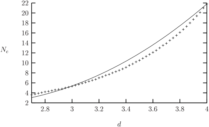
Figure 2: The full line represents the curve $N_{c}(d)$ obtained by the three-loop result improved by the constraint $N_{c}(2)=2$, Eq.(7). The crosses represent our calculation.

All these checks show the consistency between our computation and most of the previous theoretical approaches. It is in contradiction with the six loop calculation of Pelissetto et al.. Note that the result $N_{c}(3)>3$ does not exclude a priori the existence of a fixed point not analytically related — in $N$ and $\epsilon=4-d$ — to those found above $N_{c}(d)$. This is, in fact, the position advocated by Pelissetto et al. pelissetto01b . However, we have numerically searched for this fixed point with our equations without success. This implies three possibilities. The first one is that our method is not able — in principle — to find this kind of fixed point. Let us emphasize that, although it is not possible to exclude this case, it is improbable that a method which recovers all previous results in a convincing way, misses such a fixed point. Another possibility is that it has a so small basin of attraction that we have systematically missed it in our numerical investigation of our equations. This would mean that it probably does not play any role in the physics of frustrated magnets. The transitions should therefore be of first order for almost all real systems. It would then be very difficult to explain the occurence of generic weak first order phase transitions. Finally, there remains the possiblity that the fixed point does not exist at all which now appears as the most probable solution.

VI.2 Scaling without fixed and pseudo-fixed point

The hypothesis of the absence of fixed point immediately raises the theoretical challenge to explain the occurence of scaling in absence of a fixed point. For Heisenberg spins, this question has been addressed by Zumbachzumbach93 using a local potential approximation (LPA) of the Polchinski equationpolchinski84 and by the present authors beyond LPA in the framework of the effective average action methodtissier00 . It has been realized that, when $N$ is lowered from $N>N_{c}(3)$ to $N<N_{c}(3)$, although the stable fixed point disappears, there is no major change in the RG flow.

This can be understood by considering a domain ${\cal E}$ of initial conditions of the flow corresponding to all systems we are interested in — STA, STAR, $V_{N,2}$, real materials, etc — and studying the RG trajectories starting in ${\cal E}$. One finds that there exists a domain ${\cal D}\subseteq{\cal E}$ such that all trajectories emerging from ${\cal D}$ are attracted towards a small domain ${\cal R}$ in which the flow is very slow. Since the flow is very slow in ${\cal R}$ the RG time spent in this region is long and, thus, the correlation lengths of the systems in ${\cal D}$ are very large. One therefore partly recovers scaling for systems in ${\cal D}$ (that aborts only for very small reduced temperatures). Moreover, the smallness of ${\cal R}$ ensures the existence of (pseudo-)universality. Consequently ${\cal R}$ mimics a true fixed point.

This idea has been formalized through the concept of pseudo-fixed point, corresponding to the point in ${\cal{R}}$ where the flow is the slowest, the minimum of the flowzumbach93 . At this point it has been possible to compute (pseudo-)critical exponents characterizing the pseudo-scaling (and pseudo-universality) encountered in Heisenberg frustrated spin systemszumbach93 ; tissier00 .

Within our approach, we confirm the existence, for values of $N$ just below $N_{c}(3)$, of a minimum of the flow leading indeed to pseudo-scaling and quasi-universality (see Ref. tissier00, and, for details, Ref. tissier02b, ). However, when $N$ is lowered, the minimum of the flow is less and less pronounced and, for some value of $N$ between 2 and 3, it completely disappears. Since (pseudo-)scaling is observed in experiments and numerical simulations in XY systems this means that the minimum of the flow does not constitute the ultimate explanation of scaling in absence of a fixed point. At this stage, one reaches the limits of the notion of minimum of the flow as the quantity playing the role of (pseudo-)fixed point. First, it darkens the important fact that the notion relevant to scaling is not the existence of a minimum of the flow but that of a whole region ${\cal{R}}$ in which the flow is slow, i.e. the $\beta$ functions are small. Put it differently, the existence of a minimum of the flow does not guarantee that the flow is slow, i.e. that the correlation length is large compared with the lattice spacing. Reciprocally, it can happen that the RG flow is slow, the correlation length being large, and that scaling occurs even in absence of a minimum. Second, reducing $\cal{R}$ to a point, one rules out the possibility to test the violation of universality. Clearly, the degree of universality is related to the size of $\cal{R}$. The smaller $\cal{R}$ the more universal is the behavior.

Qualitatively — thanks to continuity arguments — one expects that, for $N$ close to $N_{c}(3)$, all systems in $\cal E$ exhibit pseudo-scaling — ${\cal D}={\cal E}$ — and ${\cal{R}}$ is almost pointlike so that the transitions are extremely weakly of first order and universality almost holds. When $N$ is sufficiently decreased, two phenomena occur. First, ${\cal{D}}$ gets smaller than ${\cal E}$ and thus the transitions become of strong first order for all systems that belong to ${\cal E}$ but not to ${\cal D}$. Second, ${\cal{R}}$ gets wider and thus a whole spectrum of exponents is observed and pseudo-universality breaks down. Note that these two phenomena are not obligatorily simultaneous so that, for intermediate values of $N$, scaling still holds while pseudo-universality is already significantly violated. These two phenomena are observed numerically in the Heisenberg and XY systems: STA, STAR and $V_{N,2}$ models. For $N=3$, all these models display scaling but with $\beta$ exponents that are almost incompatible [$\beta_{STA}$=0.285(11),mailhot94 $\beta_{STAR}$=0.221(9) and $\beta_{V_{3,2}}$=0.193(4) (see Ref. loison00b, )] which means that one probably starts leaving the pseudo-universal regime. For $N=2$, scaling is only observed for STA — $\beta=0.24(2)$ here — while the transitions for STAR and $V_{2,2}$ are found to be of first order.

From a theoretical point of view, the Heisenberg case has been already treated in Ref. tissier00, . We now concentrate on the XY case.

VI.3 Our results

In practice, we numerically integrate the flow equations (12) and compute physical quantities like correlation length and magnetization as a function of the reduced temperature $t_{r}=(T-T_{c})/T_{c}$. Since one expects the behavior of frustrated magnets to be nonuniversal, one should study each system independently of the others. Thus, ideally, one should consider as initial conditions of the RG flow all the microscopic parameters characterizing a specific lattice system. This program would require to identify and to deal with an infinite number of coupling constants. This remains a theoretical challenge. Rather than doing this, we have chosen to address the question of scaling in absence of a fixed point independently of a given microscopic system, using for $\Gamma_{k}$ a finite ansatz similar to, but richer than, Eq.(11).

Since our truncations forbid us to relate precisely the thermodynamical quantities to the microscopic couplings, we have chosen, as initial conditions, the simplest temperature dependence of the parameters at the scale $k=\Lambda$. This consists in fixing all coupling constants to temperature-independent values and in taking the usual ansatz for the quadratic term of $\Gamma_{k}$:

$$\kappa_{k=\Lambda}=a+b\,T$$ (17)

where $a$ and $b$ are parameters that we have varied to test the robustness of our conclusions. For each temperature we have integrated the flow equations and deduced the $t_{r}$-dependence of the physical quantities around the critical temperature.

Let us now review the main results obtained by the integration of the RG flow.

1) The integration of the flow equations leads generically to good power laws in reduced temperature for the magnetization, the correlation length (see FIG. 3) and the susceptibility. We are thus able to extract pseudo-critical exponents varying typically, for $\beta$ between 0.25 and 0.38 and for $\nu$ between 0.47 and 0.58. This phenonomenon holds for a wide domain ${\cal D}$ in coupling constant space.

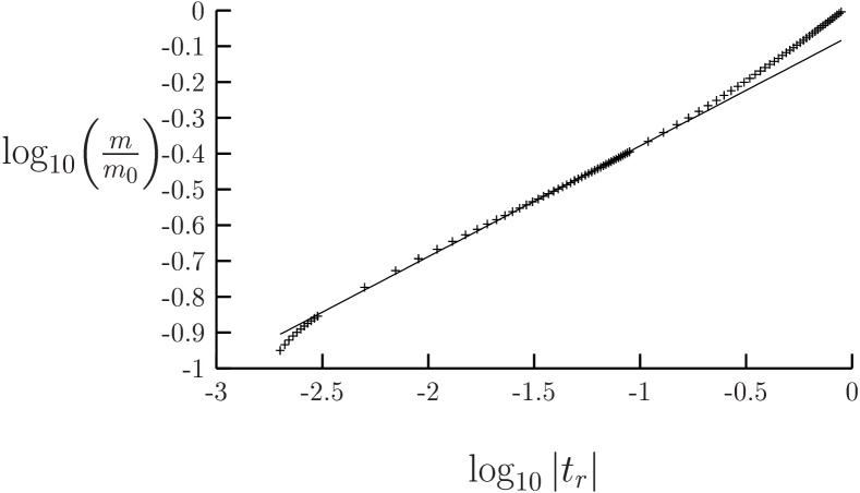
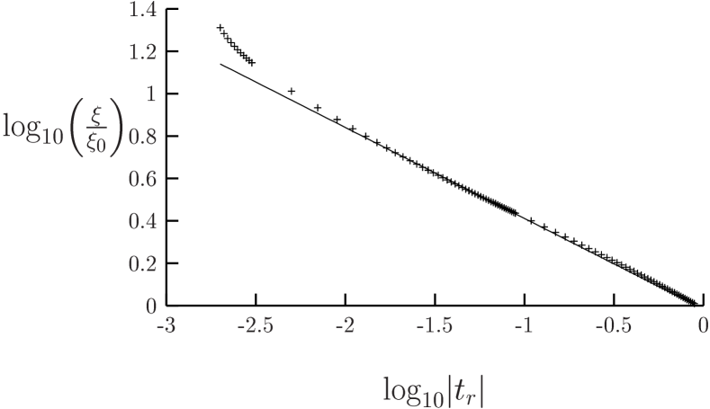
Figure 3: Log-log plots of the magnetization $m$ and of the correlation length $\xi$ for $N=2$ as functions of the reduced temperature $t_{r}$ for parameters corresponding to materials of group 1. The straight lines correspond to the best power law fit of the data. The power-law behavior observed breaks down for small $t_{r}$.

2) We easily find initial conditions leading to pseudo-exponents close to those of group 2: $\beta=0.38$, $\nu=0.58$ and $\gamma=1.13$ (see Ho and Dy in Table 1 for comparison). We have checked that the previous result is quite stable to both variations of the microscopic parameters and to a change of the $T$-dependence of the microscopic coupling constants. This is in agreement with the stability of $\beta$ in group 2. In the region of parameters leading to this behavior, correlation lengths as large as 5000 lattice spacings are found.

3) We also easily find initial conditions leading to $\beta\simeq 0.25$, corresponding to group 1. The power laws then hold on smaller range of temperature and the critical exponents are more sensitive to the determination of $T_{c}$ and to the initial conditions, in agreement with point ii) of Section III-A. For such values of $\beta$, we find a range of values of $\nu$ — $0.47\leq\nu\leq 0.49$ — which is somewhat below the value found for CsMnBr₃ (see Table 1). Also, the corresponding $\eta$ deduced from the scaling relation $\eta=2\beta/\nu-1$ is always positive and, at best, zero. Finally, it is very interesting to notice that when we find $\beta$ of order 0.25 (group 1) we also find correlation lengths at the transition of the order of a few hundreds lattice spacings which coincide rather well with the first size where a direct evidence of a first order transition has been seen in Monte Carlo RG simulations (lattice sizes around 100) itakura03 .

4) For $\beta\simeq 0.3$ we find critical exponents in good agreement with those obtained by the six-loop calculation of Ref. pelissetto01a, (see Table 1). For instance, for $\beta=0.33$ we find $\nu\simeq 0.56$ and $\gamma\simeq 1.07$.

VII Conclusion

On the basis of their specific symmetry breaking scheme it has been proposed garel76 ; yosefin85 ; kawamura88 that the critical physics of XY frustrated systems in three dimensions could undergo a second order phase transition characterized by critical exponents associated with a new universality class. We have given convincing arguments that rather favor the occurence of — generically weak — first order transitions for all XY frustrated magnets with a spreading of (pseudo-)critical exponents. This is supported by experimental and numerical results that do not agree with a second order behavior. Moreover we have shown, using a nonperturbative approach, that this generic but nonuniversal scaling finds a natural explanation in terms of slowness and “geometry” of the flow. Our approach appears to explain the main puzzling features of XY frustrated magnets.

We now propose several tests to confirm our approach. On the experimental side, more accurate determinations of critical exponents could lead to a definitive answer on the nature of the transition, at least if no drastically new physics emerges (as it could be the case for Helimagnets). In particular, it is important to check that $\eta$ is negative for CsMnBr₃, and therefore to refine the determination of $\nu$. It would also be of utmost interest to have more precise determinations of $\alpha$ in CsMnBr₃, CsNiCl₃ and CsMnI₃ which are, up to now, only marginally compatible. In case they are different, this would corroborate the lack of universality that we predict. The existence of a continuous spectrum of critical exponents could be directly tested by simulating, for example, a family of models, extrapolating continuously from STA to STAR.

On the theoretical side, it would be of interest to push the derivative expansion to refine the value of $\eta$ for group 1, which is, as usual, overestimated tetradis94 . This would allow to reproduce its observed negative value. Moreover, it would be interesting to clarify the discrepancy between the nonperturbative approach and the six loop result. The ability of our approach to reproduce exactly the whole set of exponents found by Pelissetto et al. suggests that their fixed point does not correspond to a true fixed point but, in fact, to a region where the flow is very slow. One can thus question the convergence of the perturbative result which is not Borel summable. A detailed analysis of this problem of convergence could reveal that the real fixed point found in the perturbative approach is, actually, a complex one.

Finally, the major characteristics of XY-frustrated magnets i.e. the existence of scaling laws with continuously varying exponents are probably encountered in other physical contexts, generically systems with a critical value $N_{c}$ of the number of components of the order parameter, separating a true second order behavior and a naïvely first order one.

Appendix A Threshold functions

We discuss in this appendix the different threshold functions $l_{n_{1},n_{2}}^{d}$, $m_{n_{1},n_{2}}^{d}$ and $n_{n_{1},n_{2}}^{d}$ appearing in the flow equations (12).

The threshold functions are defined as:

$$l_{n_{1},n_{2}}^{d}(w_{1},w_{2},a) =-\frac{1}{2}\int_{0}^{\infty}dy\;y^{d/2-1}\tilde{\partial}_{t}\left\{\frac{1}{(P_{1}(y)+w_{1})^{n_{1}}(P_{2}(y)+w_{2})^{n_{2}}}\right\},$$ (18a)

$$m_{n_{1},n_{2}}^{d}(w_{1},w_{2},a) =-\frac{1}{2}\int_{0}^{\infty}dy\;y^{d/2-1}\tilde{\partial}_{t}\left\{\frac{y(\partial_{y}P_{1}(y))^{2}}{(P_{1}(y)+w_{1})^{n_{1}}(P_{2}(y)+w_{2})^{n_{2}}}\right\},$$ (18b)

$$n_{n_{1},n_{2}}^{d}(w_{1},w_{2},a) =-\frac{1}{2}\int_{0}^{\infty}dy\;y^{d/2-1}\tilde{\partial}_{t}\left\{\frac{y\partial_{y}P_{1}(y)}{(P_{1}(y)+w_{1})^{n_{1}}(P_{2}(y)+w_{2})^{n_{2}}}\right\}\$$ (18c)

with:

$$P_{1}(y) =y(1+r(y)+a)$$ (19)

$$P_{2}(y) =y(1+r(y))\ .$$ (20)

In all the previous expressions $y$ is a dimensionless quantity: $y=q^{2}/k^{2}$ where $q$ is the momentum variable over which the integral in Eq.(9) is performed. As for $r(y)$, it corresponds to the dimensionless renormalized infrared cut-off:

$$r(y)=\frac{R_{k}(q^{2})}{Zq^{2}}=\frac{R_{k}(yk^{2})}{Zk^{2}y}\ .$$ (21)

In Eqs. 18a–18c, $\tilde{\partial}_{t}$ means that only the $t$-dependence of the function $R_{k}$ is to be considered and not that of the coupling constants. Therefore one has:

$$\tilde{\partial}_{t}P_{i}(y) =\frac{\partial R_{k}}{\partial t}\frac{\partial}{\partial R_{k}}P_{i}(y)$$ (22)

$$=-y(\eta r(y)+2yr^{\prime}(y)).$$ (23)

Now the threshold functions can be expressed as explicit integrals if we compute the operation of $\tilde{\partial}_{t}$. To this end, it is interesting to notice the equality: $\partial_{y}\tilde{\partial}_{t}P_{i}(y)=\tilde{\partial}_{t}\partial_{y}P_{i}(y)$, so that:

$$\tilde{\partial}_{t}\partial_{y}r=-\eta(r+yr^{\prime})-2y(2r^{\prime}+yr^{\prime\prime})$$ (24)

We then get:

$$\begin{split}l_{n_{1},n_{2}}^{d}(w_{1},w_{2},a)=-\frac{1}{2}\int_{0}^{\infty}dy\;y^{d/2}\;&\frac{\eta r+2yr^{\prime}}{(P_{1}(y)+w_{1})^{n_{1}}(P_{2}(y)+w_{2})^{n_{2}}}\left(\frac{n_{1}}{P_{1}(y)+w_{1}}+\frac{n_{2}}{P_{2}(y)+w_{2}}\right)\end{split}$$ (25)

$$\begin{split}n_{n_{1},n_{2}}^{d}(w_{1},w_{2},a)=-&\frac{1}{2}\int_{0}^{\infty}dy\;y^{d/2}\frac{1}{(P_{1}(y)+w_{1})^{n_{1}}(P_{2}(y)+w_{2})^{n_{2}}}\Bigg{\{}y(1+a+r+yr^{\prime})(\eta r+2yr^{\prime})\times\\ &\left(\frac{n_{1}}{P_{1}(y)+w_{1}}+\frac{n_{2}}{P_{2}(y)+w_{2}}\right)-\eta(r+yr^{\prime})-2y(2r^{\prime}+yr^{\prime\prime})\Bigg{\}}\end{split}$$ (26)

$$\begin{split}m_{n_{1},n_{2}}^{d}(w_{1},w_{2},a)=-&\frac{1}{2}\int_{0}^{\infty}dy\;y^{d/2}\frac{1+a+r+yr^{\prime}}{(P_{1}(y)+w_{1})^{n_{1}}(P_{2}(y)+w_{2})^{n_{2}}}\Bigg{\{}y(1+a+r+yr^{\prime})(\eta r+2yr^{\prime})\times\\ &\Bigg{(}\frac{n_{1}}{P_{1}(y)+w_{1}}+\frac{n_{2}}{P_{2}(y)+w_{2}}\Bigg{)}-2\eta(r+yr^{\prime})-4y(2r^{\prime}+yr^{\prime\prime})\Bigg{\}}\ .\end{split}$$ (27)

References

- (1) H. T. Diep, ed., Magnetic systems with competing interactions (World Scientific, 1994).
- (2) A. Pelissetto, P. Rossi, and E. Vicari, Phys. Rev. B 63, 140414 (2001).
- (3) A. Pelissetto and E. Vicari, Phys. Rep. 368, 549 (2002).
- (4) M. Tissier, B. Delamotte, and D. Mouhanna, Phys. Rev. Lett. 84, 5208 (2000).
- (5) M. Tissier, B. Delamotte, and D. Mouhanna, in preparation .
- (6) G. Zumbach, Nucl. Phys. B 413, 771 (1994).
- (7) M. Yosefin and E. Domany, Phys. Rev. B 32, 1778 (1985).
- (8) H. Kawamura, Phys. Rev. B 38, 4916 (1988).
- (9) T. Garel and P. Pfeuty, J. Phys. C: Solid St. Phys. 9, L245 (1976).
- (10) F. Pérez, T. Werner, J. Wosnitza, H. von Löhneysen, and H. Tanaka, Phys. Rev. B 58, 9316 (1998).
- (11) M. F. Collins and O. A. Petrenko, Can. J. Phys. 75, 605 (1997).
- (12) V. P. Plakhty, J. Kulda, D. Visser, E. V. Moskvin, and J. Wosnitza, Phys. Rev. Lett. 85, 3942 (2000).
- (13) P. de V. Du Plessis, A. M. Venter, and G. H. F. Brits, J. Phys.: Condens. Matter 7, 9863 (1995).
- (14) R. Deutschmann, H. von Löhneysen, J. Wosnitza, R. K. Kremer, and D. Visser, Euro. Phys. Lett. 17, 637 (1992).
- (15) D. Loison and K. D. Schotte, Euro. Phys. J. B 5, 735 (1998).
- (16) H. B. Weber, T. Werner, J. Wosnitza, H. von Löhneysen, and U. Schotte, Phys. Rev. B 54, 15924 (1996).
- (17) J. Zinn-Justin, Quantum Field Theory and Critical Phenomena (Oxford University Press, New York, 1989), pp. 151, 578, 3rd ed.
- (18) H. Kawamura, J. Phys. Soc. Japan 61, 1299 (1992).
- (19) M. L. Plumer and A. Mailhot, Phys. Rev. B 50, 16113 (1994).
- (20) E. H. Boubcheur, D. Loison, and H. T. Diep, Phys. Rev. B 54, 4165 (1996).
- (21) M. Itakura, J. Phys. Soc. Jap. 72, 74 (2003).
- (22) D. T. R. Jones, A. Love, and M. A. Moore, J. Phys. C: Solid St. Phys. 9, 743 (1976).
- (23) P. Bak, S. Krinsky, and D. Mukamel, Phys. Rev. Lett. 36, 52 (1976).
- (24) A. Pelissetto, P. Rossi, and E. Vicari, Nucl. Phys. B [FS] 607, 605 (2001).
- (25) S. A. Antonenko and A. I. Sokolov, Phys. Rev. B 49, 15901 (1994).
- (26) S. A. Antonenko, A. I. Sokolov, and V. B. Varnashev, Phys. Lett. A 208, 161 (1995).
- (27) L. P. Kadanoff, Physics 2, 263 (1966).
- (28) K. G. Wilson and J. Kogut, Phys. Rep. C 12, 75 (1974).
- (29) C. Wetterich, Phys. Lett. B 301, 90 (1993).
- (30) U. Ellwanger, Z. Phys. C 62, 503 (1994).
- (31) T. R. Morris, Int. J. Mod. Phys. A 9, 2411 (1994).
- (32) N. Tetradis and C. Wetterich, Nucl. Phys. B [FS] 422, 541 (1994).
- (33) D. Litim, Phys. Lett. B 486, 92 (2000).
- (34) J. Berges, N. Tetradis, and C. Wetterich, Phys. Rep. 363, 223 (2002).
- (35) C. Bagnuls and C. Bervillier, Phys. Rep. 348, 91 (2001).
- (36) P. Azaria, B. Delamotte, F. Delduc, and T. Jolicœur, Nucl. Phys. B [FS] 408, 485 (1993).
- (37) D. Loison, A. Sokolov, B. Delamotte, S. A. Antonenko, K. D. Schotte, and H. T. Diep, JETP Lett. 72, 337 (2000).
- (38) G. Zumbach, Phys. Rev. Lett. 71, 2421 (1993).
- (39) J. Polchinski, Nucl. Phys. B 231, 269 (1984).
- (40) A. Mailhot, M. L. Plumer, and A. Caillé, Phys. Rev. B 50, 6854 (1994).
- (41) D. Loison and K. D. Schotte, Euro. Phys. J. B 14, 125 (2000).
- (42) H. W. Blöte, E. Luijen, and J. R. Heringa, J. Phys. Math. Gen. 28, 6289 (1995).