Deceptive signals of phase transitions in small magnetic clusters

Abstract

We present an analysis of the thermodynamic properties of small transition metal clusters and show how the commonly used indicators of phase transitions like peaks in the specific heat or magnetic susceptibility can lead to deceptive interpretations of the underlying physics. The analysis of the distribution of zeros of the canonical partition function in the whole complex temperature plane reveals the nature of the transition. We show that signals in the magnetic susceptibility at positive temperatures have their origin at zeros lying at negative temperatures.

Experiments on Bose-Einstein condensation Anderson et al. (1995); Bradley et al. (1995); Davis et al. (1995) or the experimental determination of structural, electronic and thermal properties of clusters Schmidt et al. (1997, 1998, 2001) are prototypes of physical investigations of transitions in small systems. Intuitively phase transitions in such systems do exist. While the atomic structure at low temperatures is more or less rigid, at high temperatures the atoms move resembling a liquid drop. But the theoretical description is complicated since the thermodynamic functions of clusters do not show singularities at the transition point. Phase changes are seen in blurred slopes or humps. To have the physical concept of phase transitions and their properties of bulk material in mind and apply it to interpret the smooth thermodynamic functions for small systems, e.g. clusters, of a given size accordingly and assign a “first” or “second” order phase transition may be inconclusive. Despite the ambiguity in these signals, it is still reasonable to attribute an order to phase changes in small systems because fundamental differences between the kind of the transitions such as the existence of metastabilities for first-order transitions still persist. Therefore, various approaches for the classification of phase transitions in small systems have been developed which have to coincide in the thermodynamic limit and should be mathematically rigourous.

Gross et al. have proposed a microcanonical treatment, where phase transitions are distinguished by the curvature of the entropy $S(E)$ Gross (1995); Gross and Votyakov (2000). If $S(E)$ has a convex intruder, i.e. the microcanonical caloric curve $T(E)$ shows a backbending, the phase transition is assumed to be of first order. Franzosi et al. have started by investigating the topology of the potential energy surface and established a connection between topological changes and phase transitions Franzosi et al. (1999a, b). However, they are not able to determine the order of the phase transition. Recently we have proposed a classification scheme based on the distribution of zeros of the analytically continued canonical partition function $Z({\cal B})$, with ${\cal B}=\beta+i\tau$ ($\beta=1/T$), in the complex temperature plane Borrmann et al. (2000); Mülken and Borrmann (2000); Mülken et al. (2001a, b).

The basic principle of the description of phase transitions by the zeros of the partition function is the product theorem of Weierstrass and the theorem of Mittag-Leffler which relate integral functions to their zeros Titchmarsh (1964). Applying these theorems, the canonical partition function can be written as

$$Z(\beta) = \left(\frac{1}{2\pi\beta}\right)^{3N/2}\ \int{\rm d}^{3N}q\ \exp\left[-\beta V(q)\right]$$ (1)

$$= \left(\frac{1}{2\pi\beta}\right)^{3N/2}\prod_{k=-M}^{M}\left(1-\frac{\beta}{{\cal B}_{k}}\right)\exp\left(\frac{\beta}{{\cal B}_{k}}\right).$$ (2)

We assume the zeros to lie on a line with a density $\phi(\tau)\sim\tau^{\alpha}$ and to have a crossing angle $\nu$ with the plummet on the real temperature axis ($\gamma=\tan\nu$). Together with the imaginary part $\tau_{1}$ of the first zero ${\cal B}_{1}$ this leads to a distinct classification of phase transitions in small systems. For zeros perpendicular to the real axis with equal or increasing spacing, i.e., $\alpha\leq 0$ and $\gamma=0$, the transition is of first order, for $0<\alpha<1$ and arbitrary $\gamma$ as well as for $\gamma\neq 0$ and $\alpha\leq 0$ of second order, see Fig. 1. The imaginary part $\tau_{1}$ reflects the “discreteness” of the system. Thus, in the thermodynamic limit we have $\tau_{1}\to 0$ and our scheme coincides with the scheme given by Grossmann and coworkers Grossmann and Rosenhauer (1967).

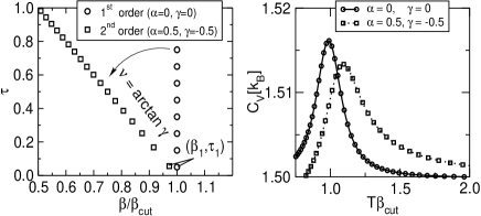
Figure 1: Examples of distributions of zeros for 1^st and 2^nd order phase transitions along with the corresponding specific heat, calculated as functions of the zeros.

We utilize small magnetic clusters exposed to an external magnetic field in order to show how the common treatment of phase transitions in small systems like the identification by humps of response functions eventually leads to misinterpretations of physical properties.

Metal clusters have the intriguing property that they occur as different isomers with almost equal ground state energies but very different magnetic moments and different geometries Borrmann et al. (1996, 1999). For simplicity, we consider in our model two isomers with magnetic moments $\mu_{1}=1\mu_{\rm B}$ and $\mu_{2}=10\mu_{\rm B}$, and their ground state energy difference $\Delta E=E_{0}(2)-E_{0}(1)=1$ meV. In the presence of an external magnetic field $H$ pointing in $z$-direction the partition function reads

$$Z(\beta)=\sum_{i=1}^{2}\exp[-\beta E_{0}(i)]\frac{2}{\beta\mu_{i}H}\sinh(\beta\mu_{i}H).$$ (3)

We have assumed equal vibrational energies. The two isomers can be identified by their average magnetic moment $\langle{\mu}\rangle$ which are calculated by standard differentiation of Eq.(3) with regard to the magnetic field

$$\langle{\mu}\rangle = \beta^{-1}\ \partial_{H}\ln Z(\beta)=\sum_{i}p_{i}\left<\mu_{i}\right>$$ (4)

$$= \sum_{i}p_{i}\;[\mu_{i}\tanh^{-1}(\beta\mu_{i}H)-1/(\beta H)],$$ (5)

where $p_{i}$ is the probability of finding isomer $i$.

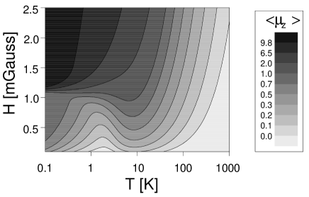
Figure 2: Contour plot af the average magnetic moment $\langle{\mu}\rangle$ versus temperature $T$ and magnetic field $H$. Note the non-linear scale.

This system is driven by two effects, the entropy increase due to thermal excitation and the alignment of the magnetic moments along the magnetic field. For low temperatures, there is a transition from $\langle{\mu}\rangle\simeq 1$ to $\langle{\mu}\rangle\simeq 10$ at about $1.1~{}$mGauss, as shown in Fig. 2. At higher temperatures the magnetic field does not align the magnetic moments along the field resulting in a general decrease of $\langle{\mu}\rangle$.

Figure 3(a) shows the occupation probability of isomer 1 ($\mu_{1}=1\mu_{B}$) for different magnetic fields. At low magnetic fields, the lower energetic isomer is predominantely occupied, while higher magnetic fields lower the ground state energy of isomer 2 ($\mu_{2}=10\mu_{B}$) and therefore the occupation is reversed. With increasing temperature the probabilities become equal. The contributions of both isomers to the total average magnetic moment $\langle{\mu}\rangle$ are plotted in Fig.3(b) and (c). At low temperatures, small magnetic fields align the magnetic moment of isomer 1 $H$. With increasing temperature the mobility of the atoms is raised which decreases the contribution of isomer 1 to $\langle{\mu}\rangle$.

From Fig. 2 and Fig. 3 we can infer that for temperatures $T\lesssim 1$ K and an increasing magnetic field a transition with a coexistence phase occurs (for coexistence in small systems see Wales and Berry (1994); Wales and Doye (1995); Berry (1999); Wales et al. (2000)). As the magnetic field is raised the contributions of both isomers to $\langle{\mu}\rangle$ are inverted which causes a bimodal probability distribution $P(\mu_{z})$ of the order parameter $\mu_{z}$. The response of the system is observable as a hump in the susceptibility $\chi=\partial_{H}\langle{\mu}\rangle$ at about $30$ K for $H=2.0$ mGauss, see Fig. 3(d).

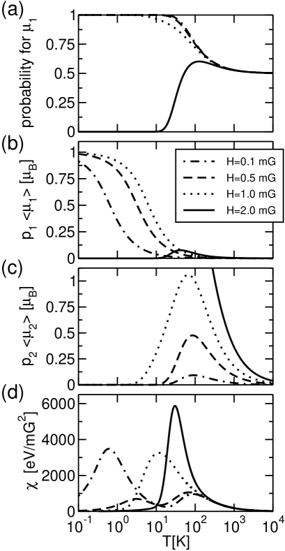
Figure 3: Plots of physical properties versus temperature $T$ for $H=0.1$, $0.5$, $1.0$, and $2.0~{}$mGauss. (a) Probability for isomer 1. (b) Contribution of isomer 1 and (c) of isomer 2 to the total average magnetic moment $\langle{\mu}\rangle$. (d) Magnetic susceptibility $\chi$.

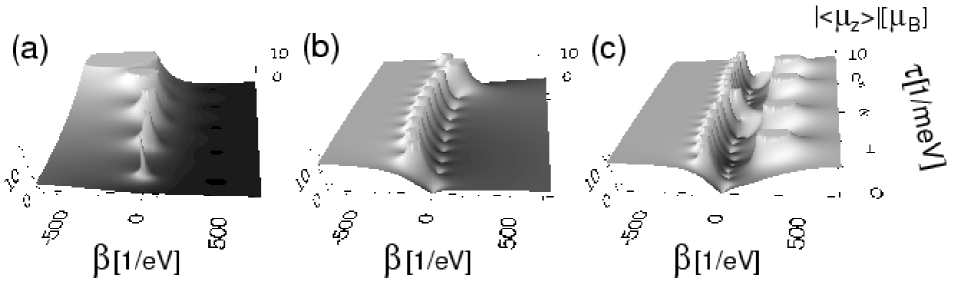
Figure 4: The absolute value of the average magnetic moment $\left|\langle{\mu}\rangle\right|$ in the complex temperature plane for (a) 0.1mGauss, (b) 1.2 mGauss, and (c) 2.0 mGauss.

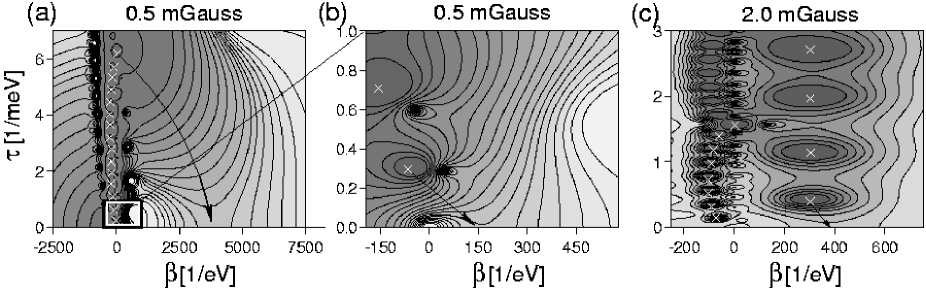
Figure 5: Contour plot of the magnetic susceptibility $\chi$ over the complex temperature plane, (a) for $H=0.5$ mGauss, (b) displays a close-up of ca. one tenth of this plane, and (c) for $H=2.0$ mGauss. The white crosses indicate the location of the poles of $\chi$. The arrows are a guide to the eye and visualize the ”radiation” of the poles.

However, at temperatures about $10-1000$ K the situation is a bit more complicated. With increasing temperature and at “intermediate” fields ($H\lesssim 1.0~{}$mGauss) the contribution of isomer 1 decreases, while the contribution of isomer 2 to $\langle{\mu}\rangle$ for is raised up to $1~{}\mu_{B}$. This also results in humps of the susceptibility $\chi$ but $P(\mu_{z})$ is unimodal because the magnetic moments of the $10\mu_{B}$ isomer are less aligned along the magnetic field. Since the first effect can be regarded as pure magnetic field driven, it is not clear whether one should attribute the humps for $H\lesssim 1.0$ mGauss to a magnetic field effect or to a temperature effect. The “coexistence” observable in the contributions of both isomers to $\langle{\mu}\rangle$ is fundamentally different, it would be more correct to associate this with thermal excitation.

Magnetic clusters are finite spin-systems. Such systems, if their energy has an upper limit, can show an inverse change of entropy with respect to energy corresponding to negative inverse temperatures, $\beta=1/T=\partial_{E}S(E)=\partial_{E}\ln\Omega(E)$ with $\Omega(E)$ being the density of states. Note, that negative temperatures are attributed to the spin temperature of the system. Negative temperatures have been measured, e.g. in LiF-crystals Purcell and Pound (1951); Ramsey (1956); Landsberg (1959) by decoupling the spin temperature from the kinetic energy contribution. The spin-lattice relaxation time is large enough (up to hours) to assure that the spin system is thermally stable and thus can come to equilibrium Abragam (1958).

Obviously, the above presented indicators of phase transition thwart the classification and to some extent the distinction between different phase transitions. Within the microcanonical ensemble the occurence of negative temperatures arises naturally because $T$ is an internal parameter in contrast to the canonical ensemble. We consider the positive and negative inverse temperatures within the canonical treatment to assure having sufficient information.

Figure 4 shows 3-dimensional images of the distribution of zeros of $Z({\cal B})$ in the complex temperature plane. The poles of $|\langle{\mu}\rangle|$ coincide with the zeros of the canonical partition function $Z({\cal B})$. For $H=0.1$ mGauss only one distribution of zeros lying at negative temperatures is present (Fig. 4(a)) corresponding to the inverse occupation of the two isomers at negative temperatures. With increasing magnetic field the shape of the distribution changes (Fig. 4(b)) and the influence of the poles of $\left|\langle{\mu}\rangle\right|$ on the real temperature axis becomes visible. While this effect is hardly seen for $H=0.1$ mGauss, one is not able to distinguish the isomers due to their real-temperature values of $\langle{\mu}\rangle$. For $H=1.2$ mGauss and $\beta>0$ the average magnetic moment equals $1\mu_{B}$, whereas we have $\langle{\mu}\rangle=10\mu_{B}$ for negative temperatures. At higher magnetic fields a second distribution of zeros corresponding to the structural transition between both isomers is seen.

An inspection of both distributions of zeros reveals that the structural transition is of first order, i.e., for the classification parameters we have $\alpha=\gamma=0$. Whereas for the transition located at negative temperatures we find $\alpha>0$ and $\gamma\neq 0$, i.e., a second-order transition, unless the magnetic field completely disappears.

Another interesting example for first-order transitions, which become second order with growing size have been found by Proykova et al. Proykova et al. (1999). There, two transitions have been found in TeF₆ clusters. They conclude that one of them is supposed to be of first-order, which becomes continuous for larger clusters, because they find two minima in the free energy as a function of an order parameter which merge to one mimimum for larger cluster sizes. The arbitrary choice of the order parameter, however, might lead to different results Wales et al. (2000).

Figure 5 displays the the magnetic susceptibility $\chi$ within the complex temperature plane. The susceptibility is plotted versus the complex inverse temperature. The blurred peaks of $\chi$ in Fig. 3(d) can be clearly related to “radiations” of the zeros onto the real axis.

An inspection of the whole complex temperature plane reveals the origin of the two maxima of the susceptibility at $H=0.5$ mGauss on the real axis (cmp. Fig. 3(d)). For $H=0.5$ mGauss the hump in $\chi$ located at $T\approx 3$ K ($\beta\approx 3800$ 1/eV) has its origin in the distribution of zeros lying at negative temperatures. Also the hump at $T=80$ K, where earlier calculations have suggested that it is also related to a structural transition Borrmann et al. (1996), has its origin in this distribution of zeros. For $2.0$ mGauss the distribution of zeros lying at positive temperatures contributes most to $\chi$ for real temperatures at $\beta\approx 400$ 1/eV $\hat{=}\;T\approx 30$ K corresponding to the structural transition seen in Fig. 3(d).

Since the distribution of poles of the considered thermodynamic function (the distribution of zeros of $Z({\cal B})$) is discrete the influences on the real axis might be shielded by zeros of these function. For example, the distributions of poles of $\langle{\mu}\rangle$ and $\chi$ are surrounded by distributions of zeros which are different for $\langle{\mu}\rangle$ and $\chi$. These thermodynamic functions are analytic everywhere except at the poles and zeros. Thus, if there is a zero in the vicinity of a pole near the real axis the decrease of $\langle{\mu}\rangle$ or $\chi$ cannot be compensated.

In conclusion we have shown that the use of the complex inverse temperature plane has advantages to common investigations of thermodynamic functions. Within our classification scheme the order of a transition can be clearly identified. By means of a simple two-isomer model for small magnetic clusters we are able to identify two different types of phase transitions. Furthermore, we found that signals in the magnetic susceptibility at positive temperatures might have their origin at negative temperatures. This also indicates that the inverse temperature is analytic at $\beta=1/T=0$ and therefore should be used in calculations of thermodynamic properties.

We thank E. R. Hilf for fruitful discussions and valuable comments.

References

- Anderson et al. (1995) M. Anderson, et al., Science 269, 198 (1995).
- Bradley et al. (1995) C. Bradley, C. Sackett, J. Tollett, and R. Hulet, Phys. Rev. Lett. 75(9), 1687 (1995).
- Davis et al. (1995) K. Davis, et al., Phys. Rev. Lett. 75(22) (1995).
- Schmidt et al. (1997) M. Schmidt, et al., Phys. Rev. Lett. 79, 99 (1997).
- Schmidt et al. (1998) M. Schmidt, B. von Issendorf, and H. Haberland, Nature 393, 238 (1998).
- Schmidt et al. (2001) M. Schmidt, et al., Phys. Rev. Lett. 86, 1191 (2001).
- Gross (1995) D. H. E. Gross, Phys. Rep. 279, 119 (1995).
- Gross and Votyakov (2000) D. H. E. Gross and E. Votyakov, E. Phys. J. B 15, 115 (2000).
- Franzosi et al. (1999a) R. Franzosi, L. Casetti, L. Spinelli, and M. Pettini, Phys. Rev. E 60, 5009 (1999a).
- Franzosi et al. (1999b) R. Franzosi, M. Pettini, and L. Spinelli, Phys. Rev. Lett. 84, 2774 (1999b).
- Borrmann et al. (2000) P. Borrmann, O. Mülken, and J. Harting, Phys. Rev. Lett. 84, 3511 (2000).
- Mülken et al. (2001a) O. Mülken, P. Borrmann, J. Harting, and H. Stamerjohanns, Phys. Rev. A 64, 013611 (2001a).
- Mülken and Borrmann (2000) O. Mülken and P. Borrmann, Phys. Rev. C 63, 023406 (2000).
- Mülken et al. (2001b) O. Mülken, H. Stamerjohanns, and P. Borrmann, Phys. Rev. E 64, 047105 (2001).
- Titchmarsh (1964) E. Titchmarsh, The Theory of Functions (Oxford University Press, 1964).
- Grossmann and Rosenhauer (1967) S. Grossmann and W. Rosenhauer, Z. Phys. 207, 138 (1967); 218, 437 (1969); S. Grossmann and V. Lehmann, ibid. 218, 449 (1969).
- Borrmann et al. (1996) P. Borrmann, B. Diekmann, E. R. Hilf, and D. Tománek, Surface Review and Letters 3, 463 (1996).
- Borrmann et al. (1999) P. Borrmann, et al., J. Chem. Phys. 111, 10689 (1999).
- Wales and Berry (1994) D. J. Wales and R. S. Berry, Phys. Rev. Lett. 73, 2875 (1994).
- Wales and Doye (1995) D. J Wales and J. P. K. Doye, J. Chem. Phys. 103, 3061 (1995).
- Berry (1999) R. S. Berry, in Theory of Atomic and Molecular Clusters, edited by J. Jellinek (Springer, Berlin , 1999).
- Wales et al. (2000) D. J. Wales, et al., Adv. Chem. Phys. 115, 1 (2000).
- Purcell and Pound (1951) E. Purcell and R. Pound, Phys. Rev. 81, 279 (1951).
- Ramsey (1956) N. Ramsey, Phys. Rev. 103, 20 (1956).
- Landsberg (1959) P. T. Landsberg, Phys. Rev. 115, 518 (1959).
- Abragam (1958) A. Abragam and W. G. Proctor, Phys. Rev. 109, 1441 (1958).
- Proykova et al. (1999) A. Proykova, R. Radev, F.-Y. Li, and R. S. Berry, Jour. Chem. Phys. 110, 3887 (1999).