Abstract

This tutorial article gives an introduction to the methods needed to treat interacting electrons in a quantum wire with a single occupied band. Since one–dimensional Fermions cannot be described in terms of noninteracting quasiparticles, the Tomonaga–Luttinger model is presented in some detail with an emphasis on transport properties. To achieve a self–contained presentation, the Bosonization technique for one–dimensional Fermions is developed, accentuating features relevant for nonequilibrium systems. The screening of an impurity in the wire is discussed, and the insight gained on the electrostatics of a quantum wire is used to describe the coupling to Fermi–liquid reservoirs. These parts of the article should be readily accessible to students with a background in quantum mechanics including second quantization. To illustrate the usefulness of the methods presented, the current–voltage relation is determined exactly for a spin–polarized quantum wire with a particular value of the interaction parameter. This part requires familiarity with path integral techniques and connects with the current literature.

Transport in Single Channel 
Quantum Wires

To appear in: Exotic States in Quantum Nanostructures  ed. by S. Sarkar, Kluwer, Dordrecht.

1 Introduction

Within the last decade there has been increased interest in the behavior of quasi one–dimensional Fermionic systems, due to significant advances in the fabrication of single channel quantum wires [goni, tarucha, yacobi] based on semiconductor heterostructures and the observation of non–Fermi liquid behavior in carbon nanotubes [delft, berkeley, basel]. While the unusual equilibrium properties of Fermions in one dimension have been studied since many decades and are well documented in review articles [solyom, voit], nonequilibrium quantum wires are an area of active research with many important question remaining to be answered.

In this article, we give a rather elementary introduction to the theoretical framework underlying much of the present studies on transport properties of one–dimensional Fermions. While we do not review extensively features of the Tomonaga–Luttinger model [tomonaga, luttinger] upon which these studies are based, we give an elementary introduction to the Bosonization technique which is an essential ingredient of current theoretical methods. We do not review the rather long history of Bosonization starting with the work by Schotte and Schotte [schotte] in 1969. Some important articles are contained in a book of reprints collected by Stone [stone]. Our approach is based on Haldane’s algebraic Bosonization [haldane], which can be understood with the usual graduate level background in physics. For a more in–depth discussion of the method, we refer to a recent review by von Delft and Schoeller [delftschoeller]. The field theoretical approach to Bosonization, which is probably harder to learn but easier to apply, has lately been expounded by Gogolin, Nersesyan and Tsvelik [gogolin].

We employ the Bosonization technique to describe a quantum wire coupled to Fermi–liquid reservoirs. In this connection the electrostatic properties of the wire play an important role. Landauer’s approach [landauer] to transport in mesoscopic systems, which is based on Fermi liquid theory, is generalized to take the electronic correlations in a single channel quantum wire into account. In the Bosonized version of the model the coupling to reservoirs is shown to be described in terms of radiative boundary conditions [eggergrabert]. This allows us to use the powerful Bosonization method also for nonequilibrium wires. About a decade ago, Kane and Fisher [kanefisher] have noted that transport properties of one–dimensional Fermions are strongly affected by impurities. Even weak impurities have a dramatic effect at sufficiently low temperatures leading to a zero bias anomaly of the conductance. It is the aim of the article to present the theoretical background necessary to study the recent literature on this subject. Again, we do not provide a review of transport properties of the Tomonaga–Luttinger model. Rather, the methods developed are illustrated by treating a particular case.

1.1 Noninteracting electrons in one dimension

Let us start by considering first noninteracting electrons of mass $m$ moving along a one–dimensional wire with a scatterer at $x=0$. For simplicity, the scattering potential is taken as a $\delta$–potential

$$V_{{\rm sc}}(x)=\frac{\hbar^{2}}{m}\,\Lambda\,\delta(x)$$ (1)

where $\Lambda$ characterizes the strength. The Schrödinger equation

$$-\,\frac{\hbar^{2}}{2m}\,\psi^{\prime\prime}(x)+\frac{\hbar^{2}}{m}\Lambda\,\delta(x)\,\psi(x)=\varepsilon\,\psi(x)$$ (2)

has for all positive energies

$$\varepsilon_{k}=\frac{\hbar^{2}k^{2}}{2m}$$ (3)

a solution ($k>0$)

$$\psi_{k}(x)=\frac{1}{\sqrt{2\pi}}\ \left\{\begin{array}[]{lll}e^{ikx}\ +r_{k}e^{-ikx}&,x<0&\\ t_{k}\ e^{ikx}&,x>0&\end{array}\right.$$ (4)

describing a wave incident from the left that is partially transmitted and partially reflected. The transmission amplitude

$$t_{k}=\frac{1}{1+i\Lambda/k}\ =\sqrt{T_{k}}\ e^{i\eta_{k}}$$ (5)

determines the transmission coefficient $T_{k}$ and the phase shift $\eta_{k}$. Likewise, there is a solution ($k>0$)

$$\psi_{-k}(x)=\psi_{k}(-x)$$ (6)

describing a wave incident from the right.

When the ends of the wire are connected to electrodes with electrical potentials $\mu_{L}$ and $\mu_{R}$, a voltage

$$U=(\mu_{L}-\mu_{R})/e$$ (7)

is applied to the wire, where $e$ is the electron charge, and an electrical current

$$I=e\ \int^{+\infty}_{-\infty}dk\,f_{k}j_{k}$$ (8)

flows. Here

$$j_{k}(x)={\rm Im}\,\psi^{*}_{k}(x)\frac{\hbar}{m}\,\frac{\partial}{\partial x}\,\psi_{k}(x)=\frac{\hbar k}{2\pi m}\,T_{k}$$ (9)

is the particle current in state $\psi_{k}$ which is independent of $x$, and the

$$f_{k} = \left\{\begin{array}[]{lll}f(\varepsilon_{k}-\mu_{L})&,k>0&\\ f(\varepsilon_{k}-\mu_{R})&,k<0&\end{array}\right.$$ (12)

with $f(\varepsilon)=1/(e^{\beta\varepsilon}+1)$ are state occupation probabilities determined by the Fermi function of the electrode from which the particles come. Both electrodes are assumed to be at the same inverse temperature $\beta$. Putting $\mu_{L,R}=\varepsilon_{F}\pm\frac{1}{2}eU$, we readily find for small voltages $U$

$$I=G\,U$$ (13)

with the conductance

$$G = e^{2}\int^{\infty}_{0}dk\,\frac{\hbar k}{2\pi m}\,T_{k}\frac{\partial}{\partial\varepsilon_{F}}\,f(\varepsilon_{k}-\varepsilon_{F})$$

$$= \frac{e^{2}}{h}\,\int^{\infty}_{0}d\varepsilon\,T(\varepsilon)\left[-\frac{\partial}{\partial\varepsilon}\,f(\varepsilon-\varepsilon_{F})\right].$$

Provided $\beta\varepsilon_{F}$ is large, this yields the Landauer formula for a single transport channel

$$G=\frac{e^{2}}{h}\,T_{F},$$ (15)

where $T_{F}$ is the transmission coefficient at the Fermi energy $\varepsilon_{F}$. If we take into account the spin degeneracy of real electrons, the conductance becomes multiplied by 2.

1.2 Fano–Anderson Model

Of course, to describe electrons in one dimension, we may also start from a tight binding model with localized electronic states at positions $x_{j}=aj$ where $a$ is the lattice constant. The Hamiltonian in the presence of an impurity at $x=0$ then takes the form of the Fano-Anderson model [fano, anderson]

$$H=\varepsilon_{0}\,a^{\dagger}_{0}a_{0}-t\sum^{+\infty}_{j=-\infty}\ (a^{\dagger}_{j+1}a_{j}+{\rm h.c.}),$$ (16)

where $t$ is the hopping matrix element and $\varepsilon_{0}>0$ is the extra energy needed to occupy the perturbed site at $x=0$. The $a_{j}$ are Fermi operators obeying the usual anti–commutation relations. This model is also exactly solvable [mahan] with eigenstates in the energy band

$$\varepsilon_{k}=-2t\cos(ka)\ ,|k|\leq\frac{\pi}{a},$$ (17)

and the transmission amplitude takes the form

$$t_{k}=\frac{1}{1+i/\lambda_{k}}\,,$$ (18)

where

$$\lambda_{k}=\frac{2t}{\varepsilon_{0}}\,\sin(ka)=\frac{\hbar v_{k}}{\varepsilon_{0}a}.$$ (19)

The last relation follows by virtue of $v_{k}=(1/\hbar)\partial\varepsilon_{k}/\partial k$. It is now easily checked that this model leads to the same result for the linear conductance than the free electron model examined previously, provided we match parameters of the unperturbed models such that the Fermi velocities $v_{F}$ at the two Fermi points coincide, and we adjust the strength of the $\delta$–function in Eq. (1) such that

$$\frac{\hbar^{2}}{m}\,\Lambda=\varepsilon_{0}a.$$ (20)

Then, we end up with the same transition coefficient $T_{F}$ at the Fermi energy.

1.3 Noninteracting Tomonaga–Luttinger model

Apparently, for low temperatures and small applied voltages, the conductance only depends on properties of states in the vicinity of the Fermi energy $\varepsilon_{F}$. We can take advantage of this fact by introducing still another model, the noninteracting Tomonaga–Luttinger (TL) model, which has the same properties near the two Fermi points $\pm k_{F}$ but is more convenient once we introduce electron interactions. Let us formally decompose the true energy dispersion curve $\varepsilon_{k}$ into two branches $+$ and $-$ of right–moving and left–moving electrons, respectively, where these branches comprise states in the energy interval $\left[\varepsilon_{F}-\Delta,\varepsilon_{F}+\Delta\right]$. (cf. Fig. 1).

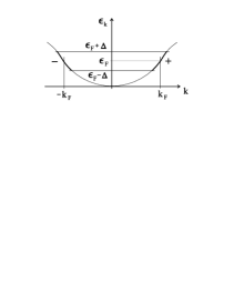
Figure 1: Physical energy dispersion curve $\epsilon_{k}$ (thin line) and the two branches $+,-$ (thick lines) of the TL model

If $\Delta$ is chosen large enough, these branches should suffice to describe the low energy physics of the true physical model, since for low temperatures and small applied voltages states with energy below $\varepsilon_{F}-\Delta$ are always occupied while states above $\varepsilon_{F}+\Delta$ are empty. The Hamiltonian of the noninteracting TL model reads

$$H=\sum_{p}\sum_{k}\,\varepsilon_{p,k}\left[c_{p,k}^{\dagger}c_{p,k}-\langle c^{\dagger}_{p,k}c_{p,k}\rangle_{0}\right].$$ (21)

Here $p=\pm$ labels the two branches. We have introduced a quantization length $L$ such that wave vectors are discrete