Multiparticle ring exchange in the Wigner glass and its possible relevance to strongly interacting two-dimensional electron systems in the presence of disorder

Abstract

We consider a two-dimensional electron or hole system at zero temperature and low carrier densities, where the long-range Coulomb interactions dominate over the kinetic energy. In this limit the clean system will form a Wigner crystal. Non-trivial quantum mechanical corrections to the classical ground state lead to multiparticle exchange processes that can be expressed as an effective spin Hamiltonian involving competing interactions. Disorder will destroy the Wigner crystal on large length scales, and the resulting state is called a Wigner glass. The notion of multiparticle exchange processes is still applicable in the Wigner glass, but the exchange frequencies now follow a random distribution. We compute the exchange frequencies for a large number of relevant exchange processes in the Wigner crystal, and the frequency distributions for some important processes in the Wigner glass. The resulting effective low energy spin Hamiltonian should be the starting point of an analysis of the possible ground state phases and quantum phase transitions between them. We find that disorder plays a crucial role and speculate on a possible zero temperature phase diagram.

I Introduction

In recent years two-dimensional electron or hole systems with very low densities are intensively studied.[1] Such systems can be generated at the interface of gallium arsenide heterostructures or silicon metal-oxide-semiconductor field effect transistors, and more recently also in organic C₆₀ and polyacene films.[2] These materials provide an excellent environment to study the effects of strong electron-electron interactions and disorder. One example is the unexpected metal-insulator transition.[1]

We consider two-dimensional electron or hole systems at zero temperature and zero magnetic field. In the absence of disorder, it is known that the system will form a Wigner crystal in the limit of very low densities, where the non-trivial correlations can be described in terms of multiparticle exchange processes.[3, 4] The exchange frequencies then determine the magnetic Hamiltonian. A calculation of the exchange frequencies of a pure two-dimensional Wigner crystal was pioneered by Roger.[5]

Although conceptually important, the pure Wigner crystal cannot be realized in the systems mentioned above, due to disorder.[6] A measure of disorder is the Drude conductance at an intermediate temperature scale at which the resistivity is relatively flat as a function of temperature, and the dominant contribution is from impurity scattering. At low densities, the measured Drude conductances are of order $e^{2}/\hbar$, indicating the importance of disorder. We consider this intermediate-temperature conductance as a tuning parameter for the quantum phase transitions to be discussed, not the asymptotic low temperature conductance. This characterization of the tuning parameter is important because, even for a pure system, the conductance at a 2D quantum critical point can be of order $e^{2}/\hbar$.[7]

It is also known that even an arbitrarily small amount of disorder will destroy the long-range order of the Wigner lattice.[8] On short length scales, however, the lattice will remain unaffected by weak disorder, so that the notion of the multiparticle exchange is still valid. Strong disorder will compromise the crystalline order even on length scales comparable to the lattice spacing. Nonetheless, the multiparticle exchange picture depends only on the existence of a rigid ground state in the classical limit (that is in the low density limit), which can be assumed to hold for any disorder strength. The exchange frequencies will, of course, follow a random distribution in the presence of disorder.

In a previous paper [9] on the metal-insulator transition, we calculated a set of relevant exchange frequencies for the clean Wigner crystal within the many dimensional WKB approximation.[10] This allowed us to conjecture a possible phase diagram in the ground state. The purpose of the present paper is to extend this calculation to the random distribution of exchange frequencies, necessarily caused by disorder in realistic situations. The resulting random and competing magnetic Hamiltonian should be an important ingredient in determining the phase diagram of this correlated complex system. A recent numerical calculation of exchange constants in a clean Wigner crystal is also available.[11]

A Wigner crystal and Wigner glass

A two-dimensional electron system with carrier density $n_{s}$ is characterized by the dimensionless parameter

$$r_{s}^{-1}=a_{B}(\pi n_{s})^{1/2},$$ (1)

which is a measure of quantum fluctuations; larger $r_{s}$ implies smaller quantum fluctuations. Here $a_{B}=\hbar^{2}\epsilon/m^{*}e^{2}$ is the effective Bohr radius; $m^{*}$ is the effective mass, and $\epsilon$ is the background dielectric constant. Thus, $r_{s}$ is the mean spacing between the carriers, in units of the Bohr radius. In a dilute system, where $r_{s}$ is large, we expect the ground state to be determined by the electrostatic repulsion between the electrons. In the absence of disorder, the classical ground state that minimizes the potential energy is a triangular lattice, the Wigner crystal.

The crystalline state can be approximately described in terms of single-particle wavefunctions that locally resemble harmonic oscillator wavefunctions. The spatial extent of these wavefunctions, $\Delta r$, depends on the oscillator frequency as $\Delta r\sim\omega_{0}^{-1/2}$, where $\omega_{0}^{2}$ is determined by the second spatial derivative of the electrostatic potential. A dimensional analysis yields $\omega_{0}\sim r_{s}^{-3/2}$, so that $\Delta r/r_{s}\sim r_{s}^{-1/4}$, and the system becomes increasingly classical as $r_{s}\to\infty$ $(n_{s}\to 0)$. At low densities, we can therefore systematically expand around the classical limit.

As the density increases, or $r_{s}$ decreases, the Wigner crystal will melt at zero temperature. The melting transition in $(d+1)$-dimension, where $d>1$, is likely to be discontinuous from Landau theory formulated in terms of the ground state energy, which must be a unique functional, $E[\rho({\bf r})]$, of the density, $\rho({\bf r})$, of the electron gas.[12] For a crystalline state, we can write

$$\langle\rho({\bf r})\rangle=\rho_{0}+\sum_{{\bf G}\neq 0}\rho_{\bf G}e^{i{\bf G}\cdot{\bf r}},$$ (2)

where $\rho_{0}$ is the average density and ${\bf G}$’s are the reciprocal lattice vectors of the crystal. In mean field theory, we can consider the ground state energy to be simply a function of the order parameters $\rho_{\bf G}$. Thus, the energy can be expanded as

$$E = E[\rho_{0}]+\frac{1}{2}\sum_{\bf G}a_{\bf G}|\rho_{\bf G}|^{2}$$ (3)

$$+ u_{3}\sum_{{\bf G}_{1},{\bf G}_{2},{\bf G}_{3}}\rho_{{\bf G}_{1}}\rho_{{\bf G}_{2}}\rho_{{\bf G}_{3}}\delta_{{\bf G}_{1}+{\bf G}_{2}+{\bf G}_{3},0}$$ (4)

$$+ u_{4}\sum_{{\bf G}_{1},{\bf G}_{2},{\bf G}_{3},{\bf G}_{4}}\rho_{{\bf G}_{1}}\rho_{{\bf G}_{2}}\rho_{{\bf G}_{3}}\rho_{{\bf G}_{4}}\delta_{{\bf G}_{1}+{\bf G}_{2}+{\bf G}_{3}+{\bf G}_{4},0}$$ (5)

$$+ \cdots$$ (6)

The quadratic term is chosen to be

$$a_{\bf G}=a(r_{s}^{c}-r_{s})+a^{\prime}(G^{2}-k_{0}^{2})^{2},$$ (7)

where $a$ and $a^{\prime}$ are positive constants and $k_{0}$ fixes the length of the reciprocal lattice vectors of the crystal. For simplicity, $u_{3}$ and $u_{4}$ were chosen to be momentum independent, but functions of $r_{s}$. On a triangular lattice, the cubic term is allowed by symmetry, hence the transition to the crystalline state is discontinuous in the order parameter, or “first order”.

Consider now the regime of the phase diagram for $r_{s}>r_{s}^{c}$ and weak disorder. We can prove that no matter how weak the disorder is the crystal falls apart at the macroscopic scale. It is sufficient to consider the limit $r_{s}\gg 1$, because quantum fluctuations can only destabilize the crystal further. We can now apply the famous Imry-Ma-Larkin[8] argument. The gain in the pinning energy due to disorder is proportional to $L^{d/2}$, whereas the cost in the elastic energy of the crystal is $L^{d-2}$, where $L$ is the linear dimension of the sample and $d$ is the space dimensionality. Thus, for $d<4$, the pinning energy wins, and the crystal is destroyed for arbitrarily small disorder. Even if the crystal is disordered in the conventional sense, it still leaves open the possibility of a power-law ordered state,[13] but this is now proven not to be possible in $d=2$.[14] The density-density correlation function falls off exponentially with a correlation length, $\xi_{D}$, given by[15]

$$\xi_{D}>R_{a}\exp[c\sqrt{\ln(R_{a}/a)}].$$ (8)

where $R_{a}$ is the length at which the displacement of the lattice becomes of the order of the lattice spacing $a$. Precise calculations of the positive constant $c$, $R_{a}$, or the prefactor are not known for the Wigner crystal. Nonetheless, $\xi_{D}$ is likely to be a large length in the limit of weak disorder, and it is safe to assume that short-range crystalline correlations will survive.

In $d=2$, the lack of crystalline order, or even a power-law crystalline order, in the presence of disorder, does not allow us to argue for a distinct state of matter distinguished by its special features with respect to the translational degrees of freedom. From this perspective, one can continuously connect the liquid state and the amorphous crystalline state by moving into the disorder plane. Thus, in $d=2$, the global symmetries that can be truly broken in the presence of disorder are the spin rotational invariance, $\cal S$, the time reversal invariance $\cal T$, and the gauge invariance $U(1)$. These symmetries can still label many distinct states of matter. For a related perspective on the problem of a pinned Wigner crystal in a magnetic field, see Ref. [16]. We note that in $d=3$ a power-law ordered Wigner glass can exist as a distinct state of matter.

B Magnetism: pure system

In discussing the magnetism of the insulating Wigner crystal, we shall ignore anharmonicities of the zero point phonon degrees of freedom, which may merely renormalize the exchange constants. The low lying magnetic Hamiltonian is due to tunneling of electrons between the lattice sites and can be expressed in terms of the $p$-particle cyclic permutaion operators $P_{1\ldots p}$. Thus,

$$H = J_{2}\sum_{\begin{picture}(17.0,10.0)(-2.0,-2.0)\put(0.0,0.0){\line(1,0){12.0}} \put(0.0,0.0){\circle*{5.0}} \put(12.0,0.0){\circle*{5.0}} \end{picture}}\left(P_{1,2}+P^{-1}\right)-J_{3}\sum_{\begin{picture}(26.0,15.0)(-2.0,-2.0)\put(0.0,0.0){\line(1,0){12.0}} \put(0.0,0.0){\line(3,5){6.0}} \put(12.0,0.0){\line(-3,5){6.0}} \put(6.0,10.0){\circle*{5.0}} \put(0.0,0.0){\circle*{5.0}} \put(12.0,0.0){\circle*{5.0}} \end{picture}}\left(P_{1,2,3}+P^{-1}\right)$$ (9)

$$+ J_{4}\sum_{\begin{picture}(26.0,15.0)(-2.0,-2.0)\put(0.0,0.0){\line(1,0){12.0}} \put(6.0,10.0){\line(1,0){12.0}} \put(0.0,0.0){\line(3,5){6.0}} \put(12.0,0.0){\line(3,5){6.0}} \put(6.0,10.0){\circle*{5.0}} \put(18.0,10.0){\circle*{5.0}} \put(0.0,0.0){\circle*{5.0}} \put(12.0,0.0){\circle*{5.0}} \end{picture}}\left(P_{1\ldots 4}+P^{-1}\right)-J_{5}\sum_{\begin{picture}(26.0,15.0)(-2.0,-2.0)\put(0.0,0.0){\line(1,0){24.0}} \put(6.0,10.0){\line(1,0){12.0}} \put(0.0,0.0){\line(3,5){6.0}} \put(18.0,10.0){\line(3,-5){6.0}} \put(6.0,10.0){\circle*{5.0}} \put(18.0,10.0){\circle*{5.0}} \put(0.0,0.0){\circle*{5.0}} \put(12.0,0.0){\circle*{5.0}} \put(24.0,0.0){\circle*{5.0}} \end{picture}}\left(P_{1\ldots 5}+P^{-1}\right)$$ (10)

$$+ J_{6}\sum_{\begin{picture}(26.0,30.0)(-2.0,-15.0)\put(6.0,10.0){\line(1,0){12.0}} \put(6.0,-10.0){\line(1,0){12.0}} \put(0.0,0.0){\line(3,5){6.0}} \put(0.0,0.0){\line(3,-5){6.0}} \put(18.0,10.0){\line(3,-5){6.0}} \put(18.0,-10.0){\line(3,5){6.0}} \put(6.0,10.0){\circle*{5.0}} \put(6.0,-10.0){\circle*{5.0}} \put(18.0,10.0){\circle*{5.0}} \put(18.0,-10.0){\circle*{5.0}} \put(0.0,0.0){\circle*{5.0}} \put(12.0,0.0){\circle*{2.0}} \put(24.0,0.0){\circle*{5.0}} \end{picture}}\left(P_{1\ldots 6}+P^{-1}\right)+\cdots.$$ (11)

The sums are over the permutations shown in this equation. There is a theorem due to Herring and Thouless that exchanges involving even number of fermions are antiferromagnetic, and those involving odd number of particles are ferromagnetic.[4] We shall follow the convention that the $J$’s are all positive.

A tractable method for calculating the exchange constants $J_{2}$, $J_{3}$, … is the instanton (or the many dimensional WKB) method. It will be shown that $J_{p}$ is

$$J_{p}=A_{p}\hbar\omega_{0}\left(\frac{S_{p}}{2\pi\hbar}\right)^{1/2}e^{-S_{p}/\hbar},$$ (12)

where $S_{p}$ is the value of the Euclidean action along the minimal action path that exchanges $p$ electrons. The quantity $\omega_{0}$ is the characteristic attempt frequency, which can be estimated from the phonon spectrum of the lattice. The prefactor $A_{p}$ is of order unity, and the Eq. (12) holds as long as $\frac{S_{p}}{\hbar}\gg 1$.

The cyclic permutation operators can be expressed in terms of the spin operators using the Dirac identity $P_{12}=\frac{1}{2}+2{\bf S}_{1}\cdot{\bf S}_{2}$ and the spin Hamiltonian is

$$H=J_{nn}\sum_{nn}{\bf S}_{i}\cdot{\bf S}_{j}+J_{nnn}\sum_{nnn}{\bf S}_{i}\cdot{\bf S}_{j}+\cdots$$ (13)

The first term in Eq. (13) is sum over distinct nearest neighbors, the second is over distinct next nearest neighbors, and so on. Here, $J_{nn}=4J_{2}+5J_{4}-4J_{3}+\cdots$ and $J_{nnn}=J_{4}+\cdots$. In general, this is a highly competing magnetic Hamiltonian. On a regular triangular lattice a model containing exchanges upto $J_{5}$ has been studied by various approximate analytical and numerical finite size (maximum of 36 sites) diagonalization methods.[17, 18] The picture that has emerged is rather complex containing a number of broken symmetry states: a ferromagnetic, a three sublattice Néel, a four sublattice Néel, and a long wavelength spiral states. In addition, on the basis of numerical work, it has been argued that a sizeable region of the phase diagram consists of a spin liquid state, with short ranged correlations, spin gap, and no broken translational and spin rotational symmetries.

C Magnetism: disordered system

In the presence of disorder, the picture should change substantially. The system is no longer described by a regular triangular lattice and will instead distort into a random lattice, with the sites dominantly determined by the pinning defects. Those properties of the pure system that are specific to a triangular lattice will no longer hold. For example, none of the antiferromagnetic states, which depend delicately on the regular lattice structure can be the true ground states. More fundamentally, there is no longer an argument that 3-particle exchange is larger than the 2-particle exchange, rather the opposite could hold, as we shall see. To explore the effect of disorder, we calculate the multiparticle exchange processes in a disordered system whose low energy magnetic Hamiltonian can be formulated as in the pure system but with a random distribution of exchange constants.

Leaving aside the gauge symmetry, the symmetries that are allowed to be broken in a disordered system are the spin rotational invariance ($\cal S$) and the time reversal invariance ($\cal T$). The phases that are potentially important are a $\cal T$-broken metal, a $\cal T$-broken insulator, a ${\cal S}$ and $\cal T$ broken spin-glass, a disordered ferromagnet, and a disordered antiferromagnet. Since a disordered system does not respect translational invariance, no further subclassification according to broken translational symmetry is possible. It is clear, however, that the regime close to the crystalline phase of the pure system will be marked by strong short-ranged crystalline order. Generically, disorder necessarily renders all quantum phase transitions between these states continuous, and thus the phase diagram is rife with quantum critical points and lines.

D The Model

The systems of experimental interest differ considerably, but they can be schematized as shown in Fig. 1.

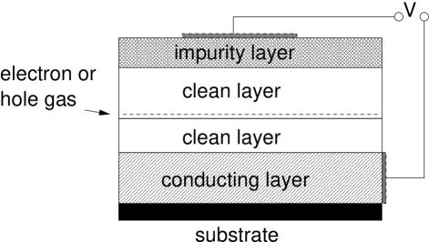
FIG. 1.: Schematic setup of the system in which a two- dimensional electron or hole gas is generated.

The carriers themselves are confined to an inversion layer or a quantum well with a width of the order of $\sim 100$Å. A buffer of several hundred Å separates the carrier plane from the doping layer, which contains impurities in the form of oppositely charged ions that provide the carriers. We will use the language appropriate to the electron-doped case for the sake of clarity; the hole-doped case can be treated identically.

Let us denote the coordinates of the $N$ electrons by ${\mathbf{r}}_{i}$, and those of the $N_{imp}$ positively charged impurities by ${\mathbf{r}}^{imp}_{j}$. We will treat the carriers as being exactly confined to the xy plane, so that ${\mathbf{r}}_{i}=(x_{i},y_{i},0)$, which means that we neglect the finite spread of the wavefunction in the direction perpendicular to the plane. This spread leads to a softening of the Coulomb potential at distances comparable with or smaller than the effective Bohr radius $a_{B}$. In the dilute limit consider here, $r_{s}\gg 1$, the many-particle wavefunction will be negligibly small in those regions of coordinate space where two or more electrons come close enough to each other to “feel” this softer potential.

We assume the only source of disorder is provided by the impurity ions in the doping layer, which is separated by a distance $d$ from the carriers. We will consider the following model for the impurity distribution: the thickness of the impurity layer is taken to be zero, so that the impurities are exactly confined to the plane $z=d$. We have also considered a second model in which we assumed the impurity layer to have a finite thickness, taken to be equal to the separation $d$ from the electron gas. Since the results are very similar, we shall not report them here.

Within the doping layer the impurities are randomly distributed. The Hamiltonian is

$$H=\sum_{i=1}^{N}\left\{\frac{{\mathbf{p}}_{i}^{2}}{2m^{*}}+\sum_{j=1}^{i-1}v\left({\mathbf{r}}_{i}-{\mathbf{r}}_{j}\right)-\sum_{j=1}^{N_{imp}}v\left({\mathbf{r}}_{i}-{\mathbf{r}}^{imp}_{j}\right)\right\},$$ (14)

where

$$v\left({\mathbf{r}}\right)=\frac{e^{2}}{\epsilon}\frac{1}{|{\mathbf{r}}|}$$ (15)

is the effective Coulomb potential, $\epsilon$ being the dielectic constant of the environment and $m^{*}$ the effective mass of the carriers.

II The Multiparticle Exchange Picture

It is useful to define the collective spatial and spin coordinates

$${\mathbf{R}}=\left({\mathbf{r}}_{1},{\mathbf{r}}_{2},\cdots,{\mathbf{r}}_{N}\right),\qquad\underline{\sigma}=\left(\sigma_{1},\sigma_{2},\cdots,\sigma_{N}\right).$$ (16)

Formally we can view ${\mathbf{R}}$ as the coordinate of a single particle moving in a $2N$-dimensional space in the potential $V({\mathbf{R}})$; see Eq. 14.

For Fermions, the partition function of the system is then

$$Z=\sum_{P\in S_{N}}(-1)^{P}\sum_{\underline{\sigma}}\int d{\mathbf{R}}\,G({\mathbf{R}},\underline{\sigma};P{\mathbf{R}},P\underline{\sigma};\beta)$$ (17)

where the first sum is over all $N!$ permutations $P{\mathbf{R}}$ of the electron coordinates, and $(-1)^{P}$ is the sign of the permutation. The propagator is defined as

$$G({\mathbf{R}}_{1},\underline{\sigma}_{1};{\mathbf{R}}_{2},\underline{\sigma}_{2};\tau)=\delta_{\underline{\sigma}_{1}\underline{\sigma}_{2}}\left\langle{\mathbf{R}}_{1},\underline{\sigma}_{1}\right|e^{-\tau H}\left|{\mathbf{R}}_{2},\underline{\sigma}_{2}\right\rangle.$$ (18)

Here $\delta_{\underline{\sigma}_{1}\underline{\sigma}_{2}}$ is a product of $N$ Kronecker delta symbols. Note that this definition of the propagator treats the electrons as distinguishable Boltzmann particles. Fermi statistics have been taken into account in the sum over boundary conditions in the partition function (17).

A The Semiclassical Approximation

The instanton method that we shall follow has been elegantly discussed by Coleman.[19] The imaginary time path integral for the propagator is ($T_{\tau}$ here denotes imaginary time)

$$G({\mathbf{R}}_{1},\underline{\sigma}_{1};{\mathbf{R}}_{2},\underline{\sigma}_{2};T_{\tau})=\delta_{\underline{\sigma}_{1}\underline{\sigma}_{2}}\int_{{\mathbf{R}}(0)={\mathbf{R}}_{1}}^{{\mathbf{R}}(T_{\tau})={\mathbf{R}}_{2}}D{\mathbf{R}}\,e^{-\frac{1}{\hbar}S[{\mathbf{R}}]},$$ (19)

where the Euclidean action is

$$S[{\mathbf{R}}]=\int_{0}^{T_{\tau}}d\tau\left\{\frac{m^{*}}{2}\left(\frac{d{\mathbf{R}}}{d\tau}\right)^{2}+V({\mathbf{R}})-V_{0}\right\}.$$ (20)

The equilibrium potential energy $V_{0}=\min_{{\mathbf{R}}}V({\mathbf{R}})$ has been subtracted out for later convenience. The stationary path satisfies

$$\frac{\delta S[{\mathbf{R}}_{c}]}{\delta{\mathbf{R}}(\tau)}=-m^{*}\frac{d^{2}{\mathbf{R}}_{c}}{d\tau^{2}}+{\vec{\nabla}}V({\mathbf{R}}_{c})=0,$$ (21)

and the action for this path is

$$S[{\mathbf{R}}_{c}]=\int_{{\mathbf{R}}_{i}}^{{\mathbf{R}}_{f}}dR\,\sqrt{2m^{*}\left(V({\mathbf{R}})-V_{0}\right)}.$$ (22)

The Planck constant enters the action in this form only through the parameter $r_{s}\sim 1/\hbar^{2}$. Therefore, the semiclassical caluclations described here are accurate in the low density limit, $r_{s}\to\infty$.

The Gaussian quantum fluctuations around the stationary path are taken into account by defining the fluctuation coordinates ${\mathbf{u}}(\tau)\equiv{\mathbf{R}}(\tau)-{\mathbf{R}}_{c}(\tau)$, in terms of which we expand the action to second order:

$$\int D{\mathbf{R}}\,e^{-\frac{1}{\hbar}S[{\mathbf{R}}]}=F\left[{\mathbf{R}}_{c}\right]e^{-\frac{1}{\hbar}S\left[{\mathbf{R}}_{c}\right]},$$ (23)

where

$$F\left[{\mathbf{R}}_{c}\right] = \int D{\mathbf{u}}\exp\left\{-\frac{1}{2\hbar}\int_{0}^{T_{\tau}}d\tau\,{\mathbf{u}}(\tau)\cdot A(\tau){\mathbf{u}}(\tau)\right\}$$ (24)

$$= \left[\det A\right]^{-1/2},$$ (25)

and we have assumed that the stationary path is unique. In cases where more than one stationary path exists, their contributions have to be summed. The differential operator $A$ is given for each path by

$$A_{\mu\nu}(\tau)=\left.-\delta_{\mu\nu}m^{*}\frac{d^{2}}{d\tau^{2}}+\frac{\partial^{2}V({\mathbf{R}})}{\partial R_{\mu}\partial R_{\nu}}\right|_{{\mathbf{R}}={\mathbf{R}}_{c}(\tau)}.$$ (26)

The determinant is defined in terms of the eigenvalues $\lambda_{\nu}$ of $A$, subject to the boundary conditions ${\mathbf{u}}(0)={\mathbf{u}}(T)=0$, as $\det A=\prod_{\nu}\lambda_{\nu}$.

B Exchange Processes and the Instanton Approximation

We will assume that there exists a definite configuration $\overline{{\mathbf{R}}}$ of the $N$ electrons that minimizes the electrostatic potential $V({\mathbf{R}})$. It is clear that this classical minimum is $N!$-fold degenerate, since the potential energy is invariant under any permutation of the electron coordinates. In the semiclassical limit, configurations where ${\mathbf{R}}$ is in the vicinity of one of these minima will contribute dominantly to the partition function. We will therefore construct stationary paths that begin and end at one of those minima. In particular, we define the instanton path ${\mathbf{R}}_{\mathrm{inst}}(\tau)$ between the two minima at $\overline{{\mathbf{R}}}_{1}$ and $\overline{{\mathbf{R}}}_{2}$ such that

$${\mathbf{R}}_{\mathrm{inst}}(-\infty)=\overline{{\mathbf{R}}}_{1}\quad\mbox{and}\quad{\mathbf{R}}_{\mathrm{inst}}(+\infty)=\overline{{\mathbf{R}}}_{2},$$ (27)

and the equation of motion (21) is satisfied. In the simplest case, that of $\overline{{\mathbf{R}}}_{1}=\overline{{\mathbf{R}}}_{2}$, the instanton path is given by ${\mathbf{R}}_{\mathrm{inst}}(\tau)\equiv\overline{{\mathbf{R}}}_{1}$. In general $\overline{{\mathbf{R}}}_{1}$ and $\overline{{\mathbf{R}}}_{2}$ differ by a permutation of the electron coordinates ${\mathbf{r}}_{i}$, so that the instanton path describes a multiparticle exchange process.

In the vicinity of a minimum, $\overline{{\mathbf{R}}}$,

$${\mathbf{R}}(\tau)-\overline{{\mathbf{R}}}\sim e^{\pm\tau\hat{\Omega}(\overline{{\mathbf{R}}})}{\mathbf{u}}_{0},$$ (28)

where ${\mathbf{u}}_{0}$ is some constant vector, and $\hat{\Omega}$ is defined as the square root of the Hessian matrix, evaluated at $\overline{{\mathbf{R}}}$:

$$\Omega^{2}_{\mu\nu}(\overline{{\mathbf{R}}})=\frac{1}{m^{*}}\left.\frac{\partial^{2}V({\mathbf{R}})}{\partial R_{\mu}\partial R_{\nu}}\right|_{{\mathbf{R}}=\overline{{\mathbf{R}}}}.$$ (29)

Hence any deviations from the classical equilibrium configuration are localized on the imaginary time axis on a scale $\delta\tau\sim\frac{1}{\omega_{a}}$, where $\omega_{a}^{2}$ is some eigenvalue (not necessarily the smallest) of $\hat{\Omega}(\overline{{\mathbf{R}}})$. In this sense, the instanton path will be localized around the location of the instanton, $\tau_{\mathrm{inst}}$, in imaginary time. On a coarse-grained time scale the exchange processes will therefore appear as instantaneous, independend events.

The instanton path will be unique in most cases. An exception is the two-particle exchange, where the electrons can take two equivalent paths corresponding to clockwise and counterclockwise exchange. This merely results in a factor of two for the exchange frequency.

The instanton formalism rests on the assumption, occasionally referred to as the dilute gas approximation, that the average distance $\Delta\tau$ on the imaginary time axis between exchange processes within the same region of space exceeds the instanton duration $\delta\tau$ by several orders of magnitude. If we consider the propagator on a time scale $T_{\tau}$ that satisfies

$$\delta\tau\ll T_{\tau}\ll\Delta\tau$$ (30)

we can make the following two crucial assumptions:

1. Each time slice contains at most one instanton event. Processes with two or more instanton events in a single time slice are of second order in $T_{\tau}/\Delta\tau$ and therefore negligible.

2. Instantons do not occur within a few instanton lengths of a time slice boundary. Again, processes that violate this assumption are of order $(T_{\tau}/\Delta\tau)(\delta\tau/T_{\tau})=\delta\tau/\Delta\tau$ and therefore negligible.

Let us now evaluate the propagator within these approximations. Since the Hamiltonian is independent of spin we will suppress the spin indices in our notation for the moment. We also define a fluctuation coordinate ${\mathbf{u}}={\mathbf{R}}-\overline{{\mathbf{R}}}$, where $\overline{{\mathbf{R}}}$ is by definition the particular minimum of $V({\mathbf{R}})$ that is closest to ${\mathbf{R}}$. Thus we want to evaluate

$$G(\overline{{\mathbf{R}}}_{1}+{\mathbf{u}}_{1};\overline{{\mathbf{R}}}_{2}+{\mathbf{u}}_{2};T_{\tau})=\int_{{\mathbf{R}}(0)=\overline{{\mathbf{R}}}_{1}+{\mathbf{u}}_{1}}^{{\mathbf{R}}(\tau_{1})=\overline{{\mathbf{R}}}_{2}+{\mathbf{u}}_{2}}D{\mathbf{R}}\,e^{-\frac{1}{\hbar}S[{\mathbf{R}}]},$$ (31)

where the deviations ${\mathbf{u}}_{1}$ and ${\mathbf{u}}_{2}$ are by assumption 2 in the quadratic regime, so that we can expand the equation of motion to linear order in ${\mathbf{u}}$. In other words, we are allowed to approximate

$$\hat{\Omega}(\overline{{\mathbf{R}}}+{\mathbf{u}})\simeq\hat{\Omega}(\overline{{\mathbf{R}}}).$$ (32)

An approximate solution of the equation of motion (21) that satisfies the boundary conditions

$${\mathbf{R}}_{c}(0)=\overline{{\mathbf{R}}}_{1}+{\mathbf{u}}_{1}\quad\mbox{and}\quad{\mathbf{R}}_{c}(T_{\tau})=\overline{{\mathbf{R}}}_{2}+{\mathbf{u}}_{2}$$ (33)

is then

$${\mathbf{R}}_{c}(\tau)=e^{-\tau\Omega_{1}^{1/2}}{\mathbf{u}}_{1}+e^{(\tau-T_{\tau})\Omega_{2}^{1/2}}{\mathbf{u}}_{2}+{\mathbf{R}}_{\mathrm{inst}}(\tau-\tau_{0}),$$ (34)

where $\tau_{0}$ is an arbitrary reference point between $0$ and $\tau_{1}$. The time derivative of each term is localized on a time scale $\delta\tau\ll T_{\tau}$, and by assumption 2 above the overlap between the three terms is exponentially small. Hence the corrections arising from the nonlinearity of the equation of motion are negligible. For the same reason the action associated with this path splits into three parts, which we write in an obvious notation as

$$S[{\mathbf{R}}_{c}]=S[{\mathbf{u}}_{1}]+S[{\mathbf{u}}_{2}]+S_{\mathrm{inst}}.$$ (35)

With the results of the previous section the propagator is then

$$G(\overline{{\mathbf{R}}}_{1}+{\mathbf{u}}_{1};\overline{{\mathbf{R}}}_{2}+{\mathbf{u}}_{2};T_{\tau})$$ (36)

$$=F\left[{\mathbf{R}}_{\mathrm{inst}}\right]\exp\left\{-\frac{1}{\hbar}\left(S[{\mathbf{u}}_{1}]+S[{\mathbf{u}}_{2}]+S_{\mathrm{inst}}\right)\right\},$$ (37)

where we already incorporated the fact that with the approximation (32) the prefactor (24) is independent of the ${\mathbf{u}}_{i}$. Let us from now on write ${\mathbf{R}}_{\mathrm{inst}}={\mathbf{R}}_{P}$ and $S_{\mathrm{inst}}=S_{P}$, where $P\in S_{N}$ labels the particular permutation that takes $\overline{{\mathbf{R}}}_{2}$ into $\overline{{\mathbf{R}}}_{1}$, i.e. $\overline{{\mathbf{R}}}_{1}=P\overline{{\mathbf{R}}}_{2}$. For later use we define the quantity $G_{P}$ as the ratio between the propagator for a given instanton path and the corresponding propagator for the trivial path ${\mathbf{R}}_{\mathrm{inst}}(\tau)\equiv\overline{{\mathbf{R}}}$, which has $S_{\mathrm{inst}}=0$. That is,

$$G_{P}:=\frac{G(\overline{{\mathbf{R}}}+{\mathbf{u}}_{1};P\overline{{\mathbf{R}}}+P{\mathbf{u}}_{2};T_{\tau})}{G(\overline{{\mathbf{R}}}+{\mathbf{u}}_{1};\overline{{\mathbf{R}}}+{\mathbf{u}}_{2};T_{\tau})}=\frac{F\left[{\mathbf{R}}_{P}\right]}{F\left[\overline{{\mathbf{R}}}\right]}e^{-\frac{1}{\hbar}S_{P}}.$$ (38)

Within the instanton approximation $G_{P}$ is independent of the fluctuation coordinates. Due to permutation symmetry all terms in $G_{P}$ are also independent of the particular choice of the minimum $\overline{{\mathbf{R}}}$.

C The Prefactor

To evaluate the prefactor (24) we would have to find a complete set of eigenfunctions ${\mathbf{u}}_{n}(\tau)$ that satisfy

$$\left[-m^{*}\delta_{\mu\nu}\partial_{\tau}^{2}+V_{\mu\nu}(\tau)\right]u_{n\nu}(\tau)=\lambda_{n}u_{n\mu}(\tau)$$ (39)

with the boundary conditions ${\mathbf{u}}_{n}(0)={\mathbf{u}}_{n}(T_{\tau})=0$. Here we used the shorthand notations $\partial_{\tau}^{2}=d^{2}/d\tau^{2}$ and $V_{\mu\nu}(\tau)=\partial^{2}V({\mathbf{R}}_{P}(\tau))/\partial R_{\mu}\partial R_{\nu}$. If we expand

$${\mathbf{u}}(\tau)=\sum_{n=0}^{\infty}c_{n}{\mathbf{u}}_{n}(\tau)$$ (40)

the path integral over ${\mathbf{u}}$ is transformed into

$$\int D{\mathbf{u}}\to\prod_{n=0}^{\infty}\int\frac{dc_{n}}{\sqrt{2\pi\hbar}}.$$ (41)

We still have to account for the possibility that one of the eigenvalues of (26) is less than or equal to zero. While it is easy to show by direct calculation that this is not the case for $F\left[\overline{{\mathbf{R}}}\right]$, a zero eigenvalue indeed exists for $F\left[{\mathbf{R}}_{P}\right]$. As an eigenfunction we consider the time derivative of the instanton path itself:

$${\mathbf{u}}_{0}(\tau):=a_{0}^{-1}\frac{d}{d\tau}{\mathbf{R}}_{P}(\tau-\tau_{0}),$$ (42)

where the normalization constant is given by

$$a_{0}^{2}=\int_{0}^{T_{\tau}}d\tau\left[\frac{d}{d\tau}{\mathbf{R}}_{P}(\tau-\tau_{0})\right]^{2}=\frac{S_{P}}{m^{*}}.$$ (43)

The last identity follows from the equation of motion (21), which can be integrated to give

$$\frac{m^{*}}{2}\left(\frac{d{\mathbf{R}}_{c}}{d\tau}\right)^{2}=V({\mathbf{R}}_{c})-V_{0},$$ (44)

which is just the Euclidean version of energy conservation. It is straightforward to verify that ${\mathbf{u}}_{0}(\tau)$ satisfies the eigenvalue equation (39) with eigenvalue $\lambda_{0}=0$. The boundary conditions ${\mathbf{u}}(0)={\mathbf{u}}(T_{\tau})=0$ are satisfied within our approximations since ${\mathbf{u}}_{0}$ is exponentially localized. This function just describes the change in ${\mathbf{R}}_{c}$ due to a change in the instanton position $\tau_{0}$, which is arbitrary within the limits $0<\tau_{0}<T_{\tau}$. Hence a shift in the instanton position corresponds to a zero mode. This is the Goldstone mode associated with broken time translation symmetry in the presence of an instanton. The change in the path ${\mathbf{R}}(\tau)={\mathbf{R}}_{P}(\tau)+{\mathbf{u}}(\tau)$ due to a change in the expansion coefficient $c_{0}$ can be related to a change in $\tau_{0}$ as follows:

$$\frac{d{\mathbf{R}}(\tau)}{dc_{0}}={\mathbf{u}}_{0}(\tau),$$ (45)

by Eq. (40), while

$$\frac{d{\mathbf{R}}(\tau)}{d\tau_{0}}=-\frac{d{\mathbf{R}}_{P}(\tau-\tau_{0})}{d\tau}=-a_{0}{\mathbf{u}}_{0}(\tau)$$ (46)

by the definition of ${\mathbf{u}}_{0}$, so that we have to replace the integration over $c_{0}$ by

$$\int\frac{dc_{0}}{\sqrt{2\pi\hbar}}\to a_{0}\int_{0}^{T_{\tau}}\frac{d\tau_{0}}{\sqrt{2\pi\hbar}}=T_{\tau}\sqrt{\frac{S_{P}}{2\pi\hbar m^{*}}}.$$ (47)

$\lambda_{0}$ is the lowest eigenvalue, since the corresponding eigenfunction is free of nodes. Hence all other eigenvalues must be positive. We now have

$$F[{\mathbf{R}}_{P}]=T_{\tau}\sqrt{\frac{S_{P}}{2\pi\hbar m^{*}}}\left(\mathrm{det}^{\prime}\left[-m^{*}\partial_{\tau}^{2}+V_{\mu\nu}(\tau)\right]\right)^{-1/2},$$ (48)

where the prime indicates that the zero eigenvalue has to be omitted in the determinant. To summarize, the prefactor is given by

$$\frac{F\left[{\mathbf{R}}_{P}\right]}{F\left[\overline{{\mathbf{R}}}\right]}=T_{\tau}\sqrt{\frac{S_{P}}{2\pi\hbar m^{*}}}\left(\frac{\det\left[-m^{*}\partial_{\tau}^{2}+V_{\mu\nu}(0)\right]}{\mathrm{det}^{\prime}\left[-m^{*}\partial_{\tau}^{2}+V_{\mu\nu}(\tau)\right]}\right)^{1/2}.$$ (49)

Let us assume that we scale all eigenmodes of the potential by the same factor $g$ and simultaneously rescale the imaginary time variable by a factor $g^{-1}$. The factors of $g$ in the determinants cancel in the numerator and in the denominator for each eigenvalue separately, and we know that the ratio of determinants cannot depend on the length $T_{\tau}$ of the time interval, except for exponentially small corrections. Hence the prefactor depends linearly on a characteristic frequency scale of $V({\mathbf{R}})$, and the ratio of determinants depends only on the relative values of the eigenfrequencies. We summarize these findings by writing $G_{P}$, defined in Eq. (38), as

$$G_{P}=T_{\tau}A_{P}\,\omega_{0}\,\sqrt{\frac{S_{P}}{2\pi\hbar}}\;e^{-\frac{1}{\hbar}S_{P}},$$ (50)

where, as stated above, $\omega_{0}$ is a characteristic frequency, and the dimensionless factor $A_{P}$ depends on the relative values of the eigenfrequencies during the exchange process. It seems reasonable to assume that $A_{P}$ is roughly of order one. Although the prefactor is not expected to cause any drastic changes in our results, it is still interesting to determine the change in characteristic frequency with disorder. It is conceivable, for example, that disorder would bring about a reduction in the phonon spectrum, and this mechanism could lead to a suppression of exchange processes.

D The Exchange Hamiltonian

Our goal in this section is a Hamiltonian description of the system in terms of multiparticle exchange operators. In the previous subsections we calculated the imaginary-time propagator on an intermediate time scale $T_{\tau}$ defined by the relation (30). To apply this result, we split the partition function (17) into $M$ imaginary time slices, where $M$ satisfies $\beta=MT_{\tau}$. This requires us to sum over $M-1$ intermediate configurations, so that the partition function reads

$$Z = \sum_{P}(-1)^{P}\sum_{\underline{\sigma}_{1}}\cdots\sum_{\underline{\sigma}_{M}}\int d{\mathbf{R}}_{1}\cdots\int d{\mathbf{R}}_{M}$$ (51)

$$\times G({\mathbf{R}}_{1},\underline{\sigma}_{1};{\mathbf{R}}_{2},\underline{\sigma}_{2};T_{\tau})$$ (53)

$$\cdots G({\mathbf{R}}_{M},\underline{\sigma}_{M};P{\mathbf{R}}_{1},P\underline{\sigma}_{1};T_{\tau}).$$

We want to make use of the quantities

$$G_{P}=\frac{G(\overline{{\mathbf{R}}}+{\mathbf{u}}_{1};P\overline{{\mathbf{R}}}+P{\mathbf{u}}_{2};T_{\tau})}{G(\overline{{\mathbf{R}}}+{\mathbf{u}}_{1};\overline{{\mathbf{R}}}+{\mathbf{u}}_{2};T_{\tau})},$$ (54)

defined in Sec. II B, which only depend on the permutation $P$, and are independent of the fluctuation coordinates ${\mathbf{u}}_{i}$ and the particular choice of the minimum $\overline{{\mathbf{R}}}$. To this end, we write the integration variables ${\mathbf{R}}_{i}$ in the form

$${\mathbf{R}}_{i}=P_{i}(\overline{{\mathbf{R}}}+{\mathbf{u}}_{i}),$$ (55)

where $\overline{{\mathbf{R}}}$ is some minimum of $V({\mathbf{R}})$, and the permutation $P_{i}$ is chosen such as to minimize the distance $|{\mathbf{R}}_{i}-P_{i}\overline{{\mathbf{R}}}|$. The integrals then have to be replaced with

$$\int d{\mathbf{R}}_{i}\to\sum_{P_{i}}\int d{\mathbf{u}}_{i},$$ (56)

where the sum is over all permutations, so that $P_{i}\overline{{\mathbf{R}}}$ covers all minima of $V({\mathbf{R}})$, and the integration over ${\mathbf{u}}_{i}$ is by construction restricted to the vicinity of ${\mathbf{u}}_{i}=0$. The partition function then reads (dropping spin in the notation for now)

$$Z = \sum_{P}(-1)^{P}\sum_{P_{1}}\cdots\sum_{P_{M}}\int d{\mathbf{u}}_{1}\cdots\int d{\mathbf{u}}_{M}$$ (57)

$$\times G\Bigl{(}P_{1}(\overline{{\mathbf{R}}}+{\mathbf{u}}_{1});P_{2}(\overline{{\mathbf{R}}}+{\mathbf{u}}_{2});T_{\tau}\Bigr{)}$$ (59)

$$\cdots G\Bigl{(}P_{M}(\overline{{\mathbf{R}}}+{\mathbf{u}}_{M});PP_{1}(\overline{{\mathbf{R}}}+{\mathbf{u}}_{1});T_{\tau}\Bigr{)}.$$

Let us now introduce the transfer matrix $\hat{T}$, defined by the relation

$$G\Bigl{(}P_{i}(\overline{{\mathbf{R}}}+{\mathbf{u}}_{i}),\underline{\sigma}_{i};P_{j}(\overline{{\mathbf{R}}}+{\mathbf{u}}_{j}),\underline{\sigma}_{j};T_{\tau}\Bigr{)}$$ (60)

$$=\left\langle i,\underline{\sigma}_{i}\right|\hat{T}\left|j,\underline{\sigma}_{j}\right\rangle\,G(\overline{{\mathbf{R}}}+{\mathbf{u}}_{i};\overline{{\mathbf{R}}}+{\mathbf{u}}_{j};T_{\tau}).$$ (61)

Comparing this definition to Eq. (54) we can easily deduce

$$\left\langle i,\underline{\sigma}_{i}\right|\hat{T}\left|j,\underline{\sigma}_{j}\right\rangle=\delta_{\underline{\sigma}_{1}\underline{\sigma}_{2}}G_{P_{ij}}=\sum_{P}G_{P}\left\langle i,\underline{\sigma}_{i}\right|\hat{P}^{\prime}\left|j,\underline{\sigma}_{j}\right\rangle,$$ (62)

where $P_{ij}=P_{i}^{-1}P_{j}$, the permutation operators $\hat{P}^{\prime}$ are defined to act only on the index $i$ as $\hat{P}^{\prime}\left|i,\underline{\sigma}\right\rangle=\left|p_{i},\underline{\sigma}\right\rangle$, and we made use of the orthogonality relation $\left\langle i,\underline{\sigma}_{i}|j,\underline{\sigma}_{j}\right\rangle=\delta_{ij}\delta_{\underline{\sigma}_{1}\underline{\sigma}_{2}}$. Thus the transfer matrix is

$$\hat{T}=\sum_{P}G_{P}\hat{P}^{\prime}.$$ (63)

Inserting Eq. (60) into the partition function (57), the latter will factorize into a fluctuation part and a tunneling part:

$$Z = Z_{0}\sum_{P}(-1)^{P}\sum_{i_{1}}\cdots\sum_{i_{M}}\sum_{\underline{\sigma}_{1}}\cdots\sum_{\underline{\sigma}_{M}}$$ (65)

$$\times\left\langle i_{1},\underline{\sigma}_{1}\right|\hat{T}\left|i_{2},\underline{\sigma}_{2}\right\rangle\cdots\left\langle i_{M},\underline{\sigma}_{M}\right|\hat{T}\hat{P}\left|i_{1},\underline{\sigma}_{1}\right\rangle$$

$$= Z_{0}\sum_{P}(-1)^{P}\sum_{i\underline{\sigma}}\left\langle i,\underline{\sigma}\right|\hat{T}^{M}\hat{P}\left|i,\underline{\sigma}\right\rangle,$$ (66)

where the permutation operator $\hat{P}$ acts on both $i$ and $\underline{\sigma}_{i}$ as $\hat{P}\left|i,\underline{\sigma}\right\rangle=\left|p_{i},P\underline{\sigma}\right\rangle$, and

$$Z_{0} = \int d{\mathbf{u}}_{1}\cdots\int d{\mathbf{u}}_{M}\,G(\overline{{\mathbf{R}}}+{\mathbf{u}}_{1};\overline{{\mathbf{R}}}+{\mathbf{u}}_{2};T_{\tau})$$ (68)

$$\cdots G(\overline{{\mathbf{R}}}+{\mathbf{u}}_{M};\overline{{\mathbf{R}}}+{\mathbf{u}}_{1};T_{\tau})$$

is the partition function for a $2N$-dimensional harmonic oscillator.

The $G_{P}$ are proportional to the lenght of a time slice $T_{\tau}=\beta/M$, see Eq. (50), with the exception of the identical permutation $P=1$, for which $G_{1}=1$. We therefore define the exchange energies $J_{P}=\frac{M}{\beta}G_{P}$, which allows us to write

$$\hat{T}^{M}=\left[1+\frac{\beta}{M}\sum_{P\neq 1}J_{P}\hat{P}^{\prime}\right]^{M}=\exp\left\{\beta\sum_{P\neq 1}J_{P}\hat{P}^{\prime}\right\}$$ (69)

in the zero-temperature limit, in which $M=\beta/T_{\tau}\to\infty$. The partition function now reads

$$Z=Z_{0}\sum_{P}(-1)^{P}\sum_{i\underline{\sigma}}\left\langle i,\underline{\sigma}\right|\exp\left\{\beta\sum_{P^{\prime}\neq 1}J_{P^{\prime}}\hat{P}^{\prime}\right\}\,\hat{P}\left|i,\underline{\sigma}\right\rangle.$$ (70)

This is the desired representation in terms of permutation operators. The exchange energies are given by Eq. (50) as

$$J_{P}=A_{P}\,\hbar\omega_{a}\sqrt{\frac{S_{P}}{2\pi\hbar}}\>e^{-\frac{1}{\hbar}S_{P}}.$$ (71)

If we expand the exponential in a power series, the orthogonality condition $\left\langle i,\underline{\sigma}|j,\underline{\sigma}\right\rangle=\delta_{ij}$ implies that all permutation operators $\hat{P}^{\prime}$ in this expansion have to combine with $P$ to the identical permutation: $\hat{P}_{1}^{\prime}\hat{P}_{2}^{\prime}\cdots\hat{P}_{n}^{\prime}\hat{P}\left|i,\underline{\sigma}\right\rangle=\left|i,P\underline{\sigma}\right\rangle$, or $P=(P_{n}^{\prime})^{-1}\cdots(P_{1}^{\prime})^{-1}$ as far as their action on $i$ is concerned. We can thus eliminate the sum over $P$ and absorb the spin permutations and the sign factor into the exponential. Then the sum over $i$ is redundant due to permutation symmetry and the partition function becomes

$$Z=N!Z_{0}\sum_{\underline{\sigma}}\left\langle\underline{\sigma}\right|\exp\left\{-\beta\sum_{P\neq 1}(-1)^{P+1}J_{P}\hat{P}^{\sigma}\right\}\left|\underline{\sigma}\right\rangle,$$ (72)

where $\hat{P}^{\sigma}$ acts on the spin variables as $\hat{P}^{\sigma}\left|\underline{\sigma}\right\rangle=\left|P\underline{\sigma}\right\rangle$. This is the partition function for a pure spin Hamiltonian

$$H_{\sigma}=\sum_{P}(-1)^{P+1}J_{P}\hat{P}^{\sigma}.$$ (73)

E Generalized Heisenberg Model

The spin permutation operators appearing in Eq. (73) can be rewritten in terms of Pauli spin operators. For example, if we denote by $\hat{P}^{\sigma}_{12}$ the permutation operator that interchanges $\sigma_{1}$ and $\sigma_{2}$,

$$\hat{P}^{\sigma}_{12} = \hat{\sigma}_{1}^{+}\hat{\sigma}_{2}^{-}+\hat{\sigma}_{1}^{-}\hat{\sigma}_{2}^{+}+\frac{1}{2}\left(\hat{\sigma}_{1}^{z}\hat{\sigma}_{2}^{z}+1\right)$$ (74)

$$= 2{\mathbf{S}}_{1}\cdot{\mathbf{S}}_{2}+\frac{1}{2},$$ (75)

leading to a Heisenberg term, as one can easily check by direct calculation of the matrix elements. Any permutation can be written as a combination of elementary transpositions, and hence as a product of spin operators. In general these products can be reduced using operator identities such as [17]

$$\hat{P}^{\sigma}_{123}+\hat{P}^{\sigma}_{321} = \hat{P}^{\sigma}_{12}+\hat{P}^{\sigma}_{23}+\hat{P}^{\sigma}_{31}-1,$$ (76)

$$\hat{P}^{\sigma}_{1234}+\hat{P}^{\sigma}_{4321} = \hat{P}^{\sigma}_{12}\hat{P}^{\sigma}_{34}+\hat{P}^{\sigma}_{14}\hat{P}^{\sigma}_{23}-\hat{P}^{\sigma}_{13}\hat{P}^{\sigma}_{24}$$ (78)

$$+\hat{P}^{\sigma}_{13}+\hat{P}^{\sigma}_{24}-1,$$

etc. Keeping only the dominant two-, three-, and four-particle exchange processes, the spin Hamiltonian becomes

$$H = (2J_{2}-4J_{3}+2J_{4})\sum_{<ij>}^{NN}{\mathbf{S}}_{i}\cdot{\mathbf{S}}_{j}+2J_{4}\sum_{<ij>}^{NNN}{\mathbf{S}}_{i}\cdot{\mathbf{S}}_{j}$$ (80)

$$+4J_{4}\sum_{<ijkl>}^{\diamond}\left(G_{ijkl}+G_{iljk}-G_{ikjl}\right),$$

where $NN$ indicates a sum over nearest-neighbor pairs, $NNN$ a sum over next-nearest neighbors, and $\diamond$ is a sum over all rhombi. $G_{ijkl}=({\mathbf{S}}_{i}\cdot{\mathbf{S}}_{j})({\mathbf{S}}_{k}\cdot{\mathbf{S}}_{l})$, where the vertices of the rhombus are labeled clockwise by the four indices. This Hamiltonian has been discussed in Secs. I B and I C.

III Numerical Techniques

A Calculation of the Action

The action (22)

$$S_{P}=\int_{\overline{{\mathbf{R}}}}^{P\overline{{\mathbf{R}}}}dR\sqrt{2m^{*}\left(V({\mathbf{R}}_{P})-V_{0}\right)}$$ (81)

depends only on a single length scale, which can be factored out. We define a dimensionless coordinate ${\mathbf{X}}=\frac{1}{a}{\mathbf{R}}$, where $a$ is the lattice constant of the ordered Wigner crystal. The unit cell of the triangular lattice is of area $A=\frac{\sqrt{3}}{2}a^{2}$, so that the density is

$$n_{s}=\frac{1}{A}=\frac{2}{\sqrt{3}}a^{-2},$$ (82)

which we use as a definition for $a$ in the presence of disorder. The parameter $r_{s}$, defined in Sec. I A, can be expressed in terms of $a$ as

$$r_{s}=\frac{3^{1/4}}{\sqrt{2\pi}}\frac{a}{a_{B}}\simeq 0.525\frac{a}{a_{B}}.$$ (83)

We define the dimensionless action $\tilde{S}_{P}$ by $\frac{1}{\hbar}S_{P}=r_{s}^{1/2}\tilde{S}_{P}.$ Then

$$\tilde{S}_{P}=\eta\int_{{\overline{{\mathbf{X}}}}}^{P{\overline{{\mathbf{X}}}}}dX\sqrt{\tilde{V}({\mathbf{X}}_{P})-\tilde{V}_{0}},$$ (84)

where

$$\tilde{V}({\mathbf{X}})=\sum_{i=1}^{N}\left\{\sum_{j=1}^{i-1}\frac{1}{\left|{\mathbf{x}}_{i}-{\mathbf{x}}_{j}\right|}-\sum_{j=1}^{N_{imp}}\frac{1}{\left|{\mathbf{x}}_{i}-{\mathbf{x}}^{imp}_{j}\right|}\right\}$$ (85)

is the dimensionless potential, $\tilde{V}_{0}$ is its minimum value, and $\eta$ is a numerical factor:

$$\eta=\sqrt{2}\left(\frac{2\pi}{\sqrt{3}}\right)^{1/4}\simeq 1.952.$$ (86)

The classical path that minimizes the action has to be found numerically. Therefore we discretize the integral in (84) using the trapezoidal rule, which leads to

$$\tilde{S} \simeq \frac{\eta}{2}\sum_{i=0}^{M-1}\left|{\mathbf{X}}_{i+1}-{\mathbf{X}}_{i}\right|$$ (88)

$$\times\left\{\sqrt{\tilde{V}({\mathbf{X}}_{i})-\tilde{V}_{0}}+\sqrt{\tilde{V}({\mathbf{X}}_{i+1})-\tilde{V}_{0}}\right\}.$$

The displacement of the participating electrons from their equilibrium positions creates dipole perturbations, which are screened out after a distance of a few lattice spacings, even in the absence of conventional screening. We can therefore restrict the number of moving particles to a relatively small value ${N_{\text{mobile}}}$ and hold all other particle coordinates fixed at their equilibrium values. Details on the errors due to the finite values of $M$ and ${N_{\text{mobile}}}$ can be found in Appendix A. Since these errors are of opposite sign, we believe that the total error for the action is no larger than $0.3\%$ in the clean system. In order to keep the distances $\left|{\mathbf{X}}_{i+1}-{\mathbf{X}}_{i}\right|$ approximately constant during the minimization process, the allowed variations in ${\mathbf{X}}_{i}$ are restricted to those satisfying $\delta{\mathbf{X}}_{i}\cdot\left(P{\overline{{\mathbf{X}}}}-{\overline{{\mathbf{X}}}}\right)=0$, thereby reducing the number of independent variables per time slice by one. Since initial $(i=0)$ and final $(i=M)$ conditions are held fixed, the action is a function of $(2N-1)(M-1)$ independent variables in its discretized form. For calculations on the clean system we took $M=16$ and ${N_{\text{mobile}}}\simeq 80$, depending on the particular exchange under consideration. The minimization thus involves around $2400$ variables. We used a variable metric (quasi-Newton) algorithm. [20] Due to the long range nature of the Coulomb potential the sum in the expression (85) for the potential energy converges very slowly, and is in fact only conditionally convergent. We therefore use the Ewald summation technique, in which the summation over the long-range part of the Coulomb potential is carried out in Fourier space. To improve the speed of the computation, we tabulated the Ewald summation formulas on a $50\times 50$ grid and calculated in-between values using bicubic interpolation. We explicitly checked that the interpolation procedure does not generate any errors comparable to the stated accuracy of the results. In this way a single minimization could be carried out in less than 10 minutes CPU time on a 400MHz Pentium II processor.

B The Prefactor

We now turn to the numerical evaluation of the prefactor (24), which we write in the form

$$F\left[{\mathbf{R}}_{c}\right] = \int D{\mathbf{u}}\;e^{-S[{\mathbf{u}}]},$$ (89)

$$S[{\mathbf{u}}] = \frac{m^{*}}{2\hbar}\int_{0}^{T_{\tau}}d\tau\>\left({\dot{\mathbf{u}}(\tau)}^{2}+{\mathbf{u}}(\tau)\cdot H(\tau){\mathbf{u}}(\tau)\right),$$ (90)

where

$$H_{\mu\nu}(\tau)=\frac{1}{m^{*}}\left.\frac{\partial^{2}V({\mathbf{R}})}{\partial R_{\mu}\partial R_{\nu}}\right|_{{\mathbf{R}}={\mathbf{R}}_{c}(\tau)}$$ (91)

is the Hessian matrix of the potential for the configuration at time $\tau$. We split the imaginary time axis into $M$ intervals, so that

$$T_{\tau}=s_{0}>s_{1}>\cdots>s_{M-1}>s_{M}=0,$$ (92)

and approximate $H(\tau)$ by a constant matrix $H_{i}$ within a given time interval $s_{i}>\tau>s_{i+1}$:

$$H_{\mu\nu}(\tau)\simeq(H_{i})_{\mu\nu}=\frac{1}{m^{*}}\left.\frac{\partial^{2}V({\mathbf{R}})}{\partial R_{\mu}\partial R_{\nu}}\right|_{{\mathbf{R}}={\mathbf{R}}_{i}},$$ (93)

where ${\mathbf{R}}_{i}=a{\mathbf{X}}_{i}$ are the points of the discretized instanton path determined in Sec. III A. The corresponding times $s_{i}$ can be calculated by inverting the equation of motion:

$$s_{i+1}-s_{i} = \int dR\left[\frac{2}{m^{*}}(V({\mathbf{R}})-V_{0})\right]^{-1/2}$$ (94)

$$\simeq \left(\frac{m^{*}}{8}\right)^{1/2}\frac{|{\mathbf{R}}_{i+1}-{\mathbf{R}}_{i}|+|{\mathbf{R}}_{i}-{\mathbf{R}}_{i-1}|}{\sqrt{V({\mathbf{R}}_{i})-V_{0}}}.$$ (95)

We can then write the prefactor in the form

$$F\left[{\mathbf{R}}_{c}\right] \simeq \int d{\mathbf{u}}_{1}G_{1}(0,{\mathbf{u}}_{1};T_{\tau}-s_{1})$$ (96)

$$\times \int d{\mathbf{u}}_{2}G_{2}({\mathbf{u}}_{1},{\mathbf{u}}_{2};s_{1}-s_{2})$$ (98)

$$\cdots G_{M}({\mathbf{u}}_{M-1},0;s_{M-1}),$$

where

$$G_{i}({\mathbf{u}}_{i},{\mathbf{u}}_{i+1};s) = \int D{\mathbf{u}}\,\exp\left\{-\frac{m^{*}}{2\hbar}\int_{0}^{s}d\tau\right.$$ (100)

$$\left.\left(\frac{d{\mathbf{u}}}{d\tau}^{2}+{\mathbf{u}}(\tau)\cdot H_{i}\,{\mathbf{u}}(\tau)\right)\right\}$$

is simply the propagator of a multidimensional harmonic oscillator and can easily be calculated. We define orthonormal eigenvectors ${\mathbf{\hat{}}{e}}^{i}_{\nu}$ and eigenvalues $\omega_{i\nu}^{2}$ satisfying

$$H_{i}\,{\mathbf{\hat{}}{e}}^{i}_{\nu}=\omega_{i\nu}^{2}\,{\mathbf{\hat{}}{e}}^{i}_{\nu}$$ (101)

(note that $\omega_{i\nu}$ can be imaginary), in terms of which

$$G_{i}({\mathbf{u}}_{1},{\mathbf{u}}_{2};s)=\left(\prod_{\nu}B_{i\nu}(s)\right)^{1/2}\times$$ (102)

$$\exp\left\{-\sum_{\nu}B_{i\nu}(s)\left[\frac{1}{2}(u_{\nu 1}^{2}+u_{\nu 2}^{2})\cosh\omega_{\nu}s-u_{\nu 1}u_{\nu 2}\right]\right\},$$ (103)

where $u_{\nu 1,2}={\mathbf{\hat{}}{e}}^{i}_{\nu}\cdot{\mathbf{u}}_{1,2}$ and

$$B_{i\nu}(s)=\frac{m^{*}\omega_{i\nu}}{\hbar\sinh\omega_{i\nu}s}.$$ (104)

The prefactor is then

$$F\left[{\mathbf{R}}_{c}\right]=\left(\prod_{i\nu}B_{i\nu}(s_{i}-s_{i-1})\right)^{-1/2}\left(\det M\right)^{-1/2},$$ (105)

where the matrix $M$ is defined as

$$M_{\mu\nu}^{ij} = \delta_{i,j}\left(A^{i}_{\mu\nu}+A^{i-1}_{\mu\nu}\right)-\left(\delta_{i,j+1}B^{i}_{\mu\nu}+\delta_{i,j-1}B^{j}_{\mu\nu}\right),$$ (106)

$$A^{i}_{\mu\nu} = \sum_{\lambda}e^{i}_{\lambda\mu}e^{i}_{\lambda\nu}\frac{m^{*}\omega_{i\lambda}}{\tanh\omega_{i\lambda}(s_{i}-s_{i-1})},$$ (107)

$$B^{i}_{\mu\nu} = \sum_{\lambda}e^{i}_{\lambda\mu}e^{i}_{\lambda\nu}\frac{m^{*}\omega_{i\lambda}}{\sinh\omega_{i\lambda}(s_{i}-s_{i-1})}.$$ (108)

Numerical evaluation of the determinant is now straightforward. The eigenvalue that corresponds to the zero mode of Sec. II C has to be omitted from the result (this eigenvalue will not be exactly zero here, due to the finite number of time slices). To this task, we replace $H(\tau)$ by $H(\tau)-\lambda$ in Eq. (89), and numerically search for the smallest value of $\lambda$ that satisfies $1/F(\lambda)=0$. We then divide the determinant by this value. The method outlined here has been tested on the problem of tunneling in a quartic potential in one dimension, which can be treated analytically; details can be found in Appendix B.

C The Disordered System

For the disordered system we have to sample over a large number of impurity distributions. After placing the impurities onto random locations in systems with $48$ to $280$ particles and periodic boundary conditions, we first minimize the potential energy of the classical electron configuration. No tabulation of the Ewald summation formulas was used in this minimization, since the classical equilibrium configuration is very sensitive to numerical errors. We cannot exclude the possibility that the minimization procedure gets trapped in a metastable configuration in the presence of strong disorder. On average, however, the properties of such a metastable state should be sufficiently similar to those of the true equilibrium state that our results will not be affected. For strong disorder, when the triangular lattice structure is compromised even on short length scales, we are also faced with the problem of identifying proper sets of nearest neighbors to participate in the exchange. This task is solved by a Delaunay triangulation of the electrons’ equilibrium coordinates. For the subsequent minimization of the discretized action only the ${N_{\text{mobile}}}=32\cdots 34$ particles closest to those participating in the exchange were allowed to move, with the remaining particles held fixed at their equilibrium positions. The number of time slices was reduced to $M=8$, so that we have to minimize over approximately $500$ independent variables. The minimization converges significantly slower than in the clean system, since the dependence of the action on the independent variables is less smooth. In the presence of strong disorder each minimization takes several minutes to carry out. Typically we generated around $250$ impurity configurations, for each of which $8$ exchange processes were chosen at random between sets of nearest neighbors anywhere on the lattice. We thus arrive at about $2000$ sample values per data point.

IV Results

A The Clean System

Here we present results for a large number of exchange processes in the absence of disorder, including all those that are relevant at low densities. The exchange paths are shown schematically in Fig. 2, and the corresponding values of the dimensionless action $\tilde{S}_{n}$ are listed in Table I. Roughly speaking, the action depends both on the number of particles involved, and on the smoothness of the exchange paths. Kinks in the path are penalized, since they lead to intermediate configurations with high potential energy. This is also the reason for the relatively high value of $\tilde{S}_{2}$. For the smoothest exchange paths with $n\geq 8$ the action increases roughly linear with $n$ (see Fig. 3). We have, approximately,

$$\tilde{S}_{n}\simeq 0.44+0.22n\qquad(n\geq 8).$$ (109)

We did not consider processes where a particle tunnels to a location other than a nearest-neighbor site, since the action for such processes will be considerably higher. The exchange frequency depends exponentially on the action, so that even a relatively small increase in $\tilde{S}$ can suppress $J$ quite substantially.

$n$	$\tilde{S}_{n}$	$n$	$\tilde{S}_{n}$	$n$	$\tilde{S}_{n}$	$n$	$\tilde{S}_{n}$
2	1.644	6b	2.134	8b	2.764	14	3.514
3	1.526	6c	2.526	9	2.410	16	3.934
4	1.662	6d	2.294	10	2.623
5	1.911	7	2.220	11	2.862
6	1.783	8	2.188	12	3.095

TABLE I.: The dimensionless action $\tilde{S}_{n}$ for various exchange processes, see Fig. 2.

FIG. 2.: The most important exchange paths (and some less important ones). The paths for $n=12,14$ and $16$ can be found by adding a ring of particles around the $n=6,8$ and $12$ diagrams, in the same way as the $n=8,9,10$ and $11$ diagrams can be derived from $n=2,3,4$ and $6$.

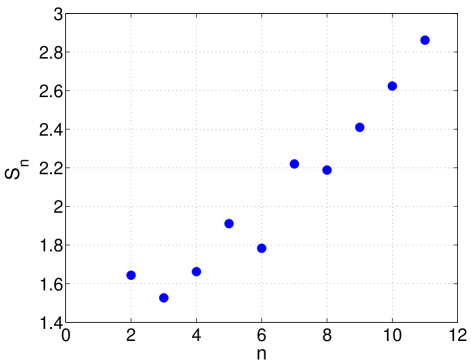
FIG. 3.: The classical action for the first ten ring exchange processes.

We define the dimensionless prefactor $\tilde{A}_{n}$ by writing

$$\frac{J_{n}}{{\text{Ry}}}=\tilde{A}_{n}\,r_{s}^{-5/4}\,\sqrt{\frac{\tilde{S}_{n}}{2\pi}}\,e^{-r_{s}^{1/2}\tilde{S}_{n}},$$ (110)

where ${\text{Ry}}=e^{2}/2\epsilon a_{B}$ is the effective Rydberg constant. In contrast to the classical action, the prefactor shows a strong dependence on the system size, as can be seen in Fig. 4. The $N$-dependence fits well to a scaling form

$$\tilde{A}_{n}(N)=a_{\infty}-\frac{a_{1}}{N}-\frac{a_{2}}{N^{2}},$$ (111)

from which we can extract the values for the infinite system: $\tilde{A}_{2}=2.60$, [21] $\tilde{A}_{3}=2.19$, $\tilde{A}_{4}=2.48$, $\tilde{A}_{5}=3.15$, and $\tilde{A}_{6}=2.90$.

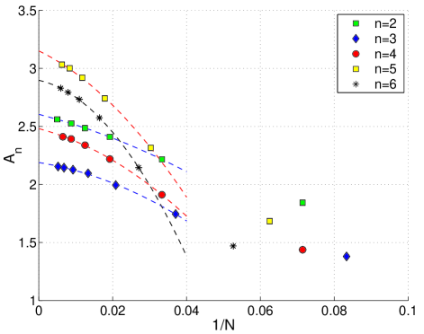
FIG. 4.: Scaling of the prefactor for two- to six-particle ring exchanges with inverse system size. $N$ is the number of particles that are allowed to move.

B Results in the Presence of Disorder

Although the technique outlined in Sec. III B allows us in principle to calculate the prefactor in the presence of impurities as well, we maintain the viewpoint that all qualitatively important changes in the exchange frequencies will be caused by variations of the classical action with disorder, and that the prefactor $A_{n}$ depends only weakly on disorder. This is by no means guaranteed, and in particular the dependence of the typical phonon frequencies on the disorder has to be investigated further. Note also that close to the melting transition anharmonicities that are not accounted for in the instanton approximation may soften the phonon modes significantly. We assume, however, that the disorder dependence of the exchange frequencies is dominated by the exponential factor. A small change in either the action or the prefactor causes a relative change

$$\frac{\delta J_{n}}{J_{n}}=\frac{\delta\tilde{A}_{n}}{\tilde{A}_{n}}+\left(\frac{1}{2}-r_{s}^{1/2}\tilde{S}_{n}\right)\frac{\delta\tilde{S}_{n}}{\tilde{S}_{n}}$$ (112)

in the exchange frequency. For moderately large values of $r_{s}$ the last term will give the dominant contribution.

To be explicit, we define the ”reduced” exchange constants

$$K_{n}:=\sqrt{\tilde{S}_{n}}\;e^{-r_{s}^{1/2}\tilde{S}_{n}}$$ (113)

and study their dependence on disorder. Figs. 5–7 show the disorder averages of $K_{n}$ for $n=2$, $3$ and $4$, normalized by their values $K_{n}^{(0)}$ for the clean system. Here $d/a$ is the distance to the impurity layer in units of the lattice constant of the clean Wigner crystal. The impurity concentration is taken to be $x=1/8$ impurity ions per electron. The system size used for determining the equilibrium configuration is $N=48$.

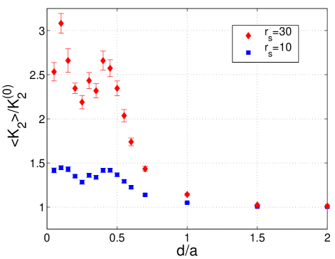
FIG. 5.: Two-particle exchange frequency relative to its value for the clean system, as a function of impurity layer distance

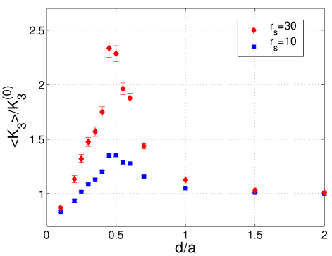
FIG. 6.: Three-particle exchange frequency relative to its value for the clean system, as a function of impurity layer distance

While the impurities are practically of no effect for $d/a\gtrsim 1$, in each case we see an enhancement of the average exchange frequency by up to a factor of $3$ (at $r_{s}=30$; at lower carrier densities the enhancement will be considerably larger) at $d/a\simeq 0.5$. For smaller values of $d/a$ three- and four-particle exchange frequencies decline again, and for $d/a\to 0$ $K_{3}$ even falls below its original value. In the following we give an interpretation of these results; more details on the frequency distribution can be found in Appendix C.

In Fig. 8 we show the deviation of the electrons’ equilibrium configuration from the ordered lattice, due to disorder. The average (static) root mean square displacement shows a sharp increase around the same value $d/a\simeq 0.5$ at which the exchange frequencies peak. We claim that both signatures are due to a structural crossover that will be investigated in more detail in the following section. In the crossover region fluctuation effects are amplified, which results in a softening of the potential barriers and an increase in the variance of the action of a instanton process. The increase in variance leads to an increase of the average exchange frequency, due to the positive curvature of $J_{n}(\tilde{S})$.

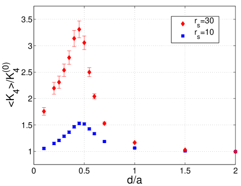
FIG. 7.: Four-particle exchange frequency relative to its value for the clean system, as a function of impurity layer distance

While three-and four-particle exchange frequencies fall off as we decrease $d/a$ below $0.5$, $K_{2}$ remains enhanced by a factor of about $2.5$ with respect to the clean system. Hence, if the distance to the impurity layer becomes very small, the two-particle exchange will dominate the magnetic properties and enhance antiferromagnetic correlations. Of course antiferromagnetic order can be realized only locally. Nevertheless, this raises the possibility of a magnetic crossover signature that can, in principle, be picked up experimentally.

Presumably this enhancement of the two-particle exchange frequency is due to impurities mediating spin singlet correlations between the electrons of the Wigner glass (see also the next section). If an electron is trapped by an impurity charge, its repulsive interaction with neighboring electrons will be greatly reduced by the impurity potential. Therefore exchange paths in which a second electron moves very close will not be suppressed as much in the partition function. Unless the impurity concentration is very high ($x\simeq 1$), this mechanism will not apply to $n>2$ exchange processes.

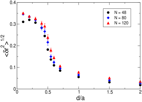
FIG. 8.: Root mean square displacement of the electrons from their equilibrium positions, due to disorder. The three curves are for different system sizes.

V The Structural Crossover

For large $d/a$ the influence of the impurities is weak, and on a local scale the lattice will be only slightly distorted (Fig. 9). In the opposite limit ($d/a\to 0$), some electrons will be trapped in the potential wells created by impurity charges. These electrons are effectively removed from the lattice. The electron-impurity pairs now appear as dipoles with a dipole strength proportional to $d$, and therefore the effective disorder strength decreases as $d$ becomes smaller. The remaining electrons will rearrange themselves to form a local Wigner lattice with an electron density less than that of the clean system (Fig. 10). In the classical limit, and for $d$ exactly equal to zero, the remaining electrons again form a perfect Wigner crystal, but with its electron density reduced by a factor $1-x$, where $x$ is the impurity concentration.

The two limits $d/a=\infty$ and $d/a=0$ therefore correspond to two distinct structural phases of the system, with different translational symmetries. However, no phase transition involving these symmetries can occur at any finite value of $d/a$. It has been known for a long time that disorder destroys any spatial long-range order in two-dimensional systems, [8] and more recently it has been shown that quasi-long range order, such as in a Bragg glass, cannot survive either. [14] To confirm the absence of long range order we show in Fig. 11 the dependence of the rms deviations on the system size for weak disorder. The deviations increase linearly with the particle number, hence quadratically in the linear dimensions.

Locally, however, we can observe a sharp crossover between the two structural “phases”. The correlation length will be strongly enhanced in the crossover region, but will remain finite due to a long distance cutoff imposed by disorder. This enhancement of the correlation length will give rise to similar effects as are usually connected with phase transitions, such as the softening of phonon modes and enhancement of fluctuations. Of course these effects can only be observed locally.

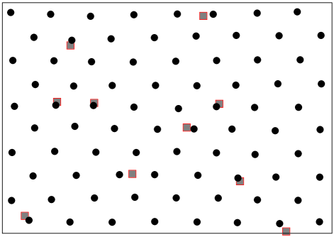
FIG. 9.: Snapshot of the classical equilibrium electron configuration at $d/a=0.7$. The filled circles show the electron positions, while the checked squares indicate the locations of the impurities.

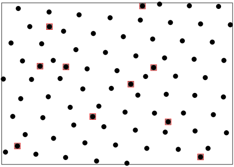
FIG. 10.: Snapshot of the classical equilibrium electron configuration at $d/a=0.1$. The filled circles show the electron positions, while the checked squares indicate the locations of the impurities.

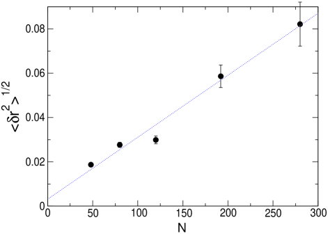
FIG. 11.: rms deviation of electron coordinates from their equilibrium positions, due to disorder, at $d/a=2$, for various system sizes. The dotted line is a least-square fit.

VI Conclusions

We have attempted to characterize the effective low energy spin Hamiltonian for a disordered Wigner crystal, or a Wigner glass and have shown that disorder can make a qualitative difference. In particular, disorder can cause an enhancement of the two-particle exchange frequency relative to the other exchange frequencies, thereby making a possible ferromagnetically ordered state less likely and a spin liquid phase more likely. The solution of such a complex, competing multiparticle spin Hamiltonian including disorder is a formidable many body problem. Nonetheless, it would be surprising if this Hamiltonian did not exhibit a multiplicity of competing phases in the ground state. We now present a speculative phase diagram in the $r_{s}$ vs. disorder plane (see Fig. 12), based primarily on symmetry considerations that can provide some guidance in the future.

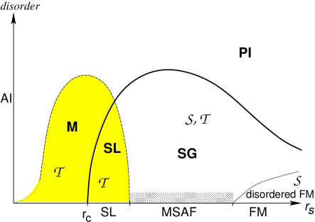
FIG. 12.: Speculative phase diagram in the $r_{s}$ - disorder plane. The various phases are: Anderson insulator (AI), paramagnetic (Efros-Shklovskii) insulator (PI), spin glass (SG), spin liquid (SL), various multi-sublattice antiferromagnetic states (MSAF), ferromagnet (FM), and a metallic state with broken time-reversal symmetry (M). The diagonally shaded area is a crossover region with intermediate-range MSAF correlations. $\cal S$ and $\cal T$ indicate broken spin-rotational and time-reversal symmetry, respectively. Not included is a possible superconducting state with broken $U(1)$ symmetry.

Let us first focus on the zero disorder axis: In the limit of very low densites ($r_{s}\to\infty$), three-particle exchange will be most relevant, leading to a state with ferromagnetic long-range order (FM).[3] Upon increasing the density, two- and four-particle exchange will frustrate the ferromagnet, until ferromagnetic order disappears at a critical density $r_{F}$. Within a mean-field approximation, the (truncated) effective spin Hamiltonian can exhibit a variety of multi-sublattice antiferromagnetic phases (MSAF).[17] There is also the possibility of a spin liquid phase (SL).[18] For even higher densities, the Wigner crystal will quantum melt at $r_{s}=r_{c}$.

While the ferromagnet with disorder averaged order parameter $\overline{<{\mathbf{S}}_{i}>}\neq 0$ can survive in the presence of weak disorder, the various MSAF states are tied to the existence of translational symmetry. As noted earlier, crystalline order will be destroyed on long length scales by any amount of disorder in two dimensions. Hence, no multi-sublattice antiferromagnetic phases can exist in the disordered system. Similarly, various dimerized broken symmetry states cannot be distinct states of matter either.[22] We expect a crossover region, with short-range antiferromagnetic correlations, to a spin glass phase (SG) at $T=0$, although there may not be a finite temperature spin glass transition in $d=2$. (In fact, numerical finite-size diagonalizations in simpler randomly frustrated spin-1/2 nearest neighbor Heisenberg models have been argued to exhibit spin glass behavior in the ground state.[23]) The complexity of this problem can be visualized by the fact that quenched disorder in such a frustrated multiparticle exchange Hamiltonain at $T=0$ appears as infinitely long ranged correlated disorder in the imaginary time direction in the field theoretical description. In any case, the spin glass phase should be characterized by a nonvanishing Edwards-Anderson order parameter, that is, the disorder average $\overline{<{\mathbf{S}}_{i}>^{2}}$ is nonzero, but $\overline{<{\mathbf{S}}_{i}>}=0$.

It is also interesting to construct a chiral order parameter. Let ${\mathbf{R}}_{1}$, ${\mathbf{R}}_{2}$, and ${\mathbf{R}}_{3}$ be the vertices of a triangular plaquette and define $\Phi({\mathbf{R}})=\langle{\mathbf{S}}({\mathbf{R}}_{1})\cdot{\mathbf{S}}({\mathbf{R}}_{2})\times{\mathbf{S}}({\mathbf{R}}_{3})\rangle$, where ${\mathbf{R}}$ is the center of the triangle. In the spin glass phase, $\overline{\Phi({\bf R})}=0$, but parasitically $\overline{\Phi^{2}({\bf R})}\neq 0$. This suggests a transition to an adjacent phase in which the Edwards-Anderson order parameter is zero, but $\overline{\Phi^{2}({\bf R})}\neq 0$. This is a new state of matter with broken time reversal symmetry, which we shall label to be the random flux state. It is interesting to ask what a prototype model could be. It is tempting to speculate that this is a variant of the random flux model. Although there is some evidence of a metal-insulator transition in the random flux model, separating a $\cal T$-broken metallic state from a $\cal T$-broken insulating state, the evidence to the contrary also exists.[24] The resolution of this controversy should be an important advance.

Next, we look at the strong-disorder, low-density region. Since the exchange frequencies decrease exponentially with $r_{s}^{1/2}$, the characteristic energy scale of disorder will be the largest energy scale, so that the carriers are independently trapped in some minima of the disorder potential. The resulting state will be a paramagnetic (Efros-Shklovskii) insulator. Since no symmetries are broken in this state, it can be continuously connected to the noninteracting disordered electron system, which is an Anderson insulator.

A superconducting state with broken $U(1)$ symmetry [25] is possible in principle. It is not clear to us, however, where in the phase diagram such a superconducting state should occur, therefore it is not included in the phase diagram shown in Fig. (12). We certainly do not imply that such a phase is impossible.

In none of the phases involving broken $\cal T$ and $\cal S$, the impurity potential can couple to the order parameter as a “random field”. Rather, the effect of the potential scattering due to impurities is to randomize the exchange constants. Similar to rigorous results known in classical statistical mechanics,[26] we can argue that these broken symmetry transitions in the ground state are necessarily continuous.[27] Thus, scaling must hold at these quantum phase transitions, and the signature of quantum criticality should be observable at finite, but low temperatures. In contrast, the Wigner crystal transition of a pure system is a first order transition at which scaling could not possibly hold.

A Accuracy Issues

In Table II we see how the classical action depends on the number of time slices $M$ used in the discretized form (88). We use the three-particle exchange, with 27 mobile particles, as an example. The errors for other exchange processes are comparable. Extrapolating to $M=\infty$ yields $\tilde{S}_{3}\simeq 1.5848$. Errors are given with respect to this value.

$M$	$\tilde{S}_{3}$	err
2	1.1924	-25%
4	1.4919	-5.9%
6	1.5455	-2.5%
8	1.5638	-1.3%
12	1.5763	-.54%
16	1.5804	-.28%
32	1.5840	-.05%

TABLE II.: Dependence of the classical action on the number of time slices used in the calculation.

Table III shows the dependence on the number of particles allowed to move in the exchange. Here $L$ is the number of layers added around the interchanging particles. The number of time slices is $M=12$. Extrapolation to $L=\infty$ yields $\tilde{S}_{3}\simeq 1.5558$. Since the errors introduced by finite $M$ and finite ${N_{\text{mobile}}}$ are of opposite sign, the choices $M=16$ and ${N_{\text{mobile}}}\simeq 80$ for the clean system should yield accurate results to within $\sim 0.2$ percent. For the disordered system, where we used $M=8$ and ${N_{\text{mobile}}}\simeq 32$, we expect the systematic errors to be on the order of $1$ percent.

${N_{\text{mobile}}}$	$L$	$\tilde{S}_{3}$	err
3	0	1.93334	24%
12	1	1.65910	6.6%
27	2	1.57627	1.3%
46	3	1.56166	.38%
69	4	1.55762	.11%
96	5	1.55628	.03%

TABLE III.: Dependence of the classical action on the number of electrons allowed to move.

B Prefactor in One Dimension

Here we apply the method introduced in Sec. III B for numerical calculation of the prefactor to tunneling in a double well potential in one dimension, which can be solved exactly. This serves as a useful test for the validity of the technique. The double well potential is given by

$$V(x)=(x^{2}-1)^{2},$$ (B1)

and the mass of the particle is set to $m=1$. According to Ref. [19], a general expression for the prefactor $P$ in one dimension is

$$P^{-2}=\frac{2}{\Lambda_{0}}e^{-\omega_{0}T_{\tau}},$$ (B2)

where $T_{\tau}$ is the length of the time slice (we set $T_{\tau}\to\infty$ at the end of the calculation) and $\omega_{0}=\sqrt{d^{2}V/dx^{2}}|_{x=1}$ is the attempt frequency. $\Lambda_{0}$ is the lowest eigenvalue of the equation

$$\left[-\partial_{\tau}^{2}+V(x(\tau))\right]u(\tau)=\Lambda u(\tau),$$ (B3)

which is given by[19]

$$\Lambda_{0}=\frac{4\omega_{0}}{S_{\mathrm{inst}}}A^{2}e^{-\omega_{0}T},$$ (B4)

where $S_{\mathrm{inst}}=\int dx\sqrt{2V(x)}$ is the action along the classical trajectory, and $A$ is the prefactor for the asymptotic form of the first time derivative of the classical trajectory:

$$\dot{x}_{c}(\tau)\simeq Ae^{-\omega_{0}|\tau|}\;\;\mbox{as}\;\;\tau\to\pm\infty.$$ (B5)

Integrating the equation of motion (21) yields

$$x_{c}(\tau)=\tanh{\sqrt{2}\tau}.$$ (B6)

From Eqs. (B2), (B4) and (B6) we immediately get

$$P=4\sqrt{6}\simeq 9.798.$$ (B7)

Table IV shows results of a numerical computation using $M$ time slices.

$M$	$4$	$8$	$16$	$32$	$64$	$128$
$A$	$10.25$	$9.970$	$9.859$	$9.819$	$9.804$	$9.799$

TABLE IV.: Prefactor in the double well problem for different numbers of time slices.

We see that the technique reproduces the exact result within one percent accuracy for $M\geq 16$.

C Distribution of Exchange Frequencies

The dimensionless action $\tilde{S}_{n}$ that enters the expression (113) for the exchange frequencies depends on the particular realization of disorder, and can therefore be viewed as a random variable. In most regions of parameter space the random distribution turns out to be well-described by a normal distribution

$$P(\tilde{S}_{n})\simeq\frac{1}{\sqrt{2\pi}\sigma_{n}}e^{-\frac{(\tilde{S}_{n}-\bar{S}_{n})^{2}}{2\sigma_{n}^{2}}}.$$ (C1)

In this approximation, the frequency distribution of $\tilde{S}_{n}$, and thereby of $K_{n}$, can be reconstructed from two parameters, the mean action $\bar{S}_{n}$ and the standard deviation $\sigma_{n}$, which are listed in Table V for various disorder strengths.

For $d/a\lesssim 0.1$ the random distribution acquires a significant non-gaussian component, hence the corresponding values are not listed.

$d/a$	$\bar{S}_{2}$	$\sigma_{2}$	$\bar{S}_{3}$	$\sigma_{3}$	$\bar{S}_{4}$	$\sigma_{4}$
2.0	1.631	0.025	1.521	0.016	1.662	0.023
1.5	1.633	0.043	1.519	0.031	1.659	0.042
1.0	1.627	0.089	1.514	0.066	1.649	0.083
0.7	1.621	0.144	1.501	0.120	1.626	0.138
0.6	1.614	0.171	1.490	0.153	1.600	0.177
0.5	1.587	0.210	1.487	0.185	1.588	0.231
0.4	1.586	0.227	1.513	0.184	1.627	0.258
0.3	1.572	0.234	1.533	0.189	1.678	0.290
0.2	1.598	0.254	1.569	0.189	1.725	0.297

TABLE V.: Dependence of mean and standard deviation of the dimensionless action on disorder strength.

REFERENCES

- [1] E. Abrahams, S. V. Kravchenko, and M. P. Sarachik, Rev. Mod. Phys. 73, 251 (2001) and references therein.
- [2] J. H. Schön, Ch. Kloc, and B. Batlogg, Science 288, 2338 (2000) and Nature 408, 549 (2000).
- [3] C. Herring, in Magnetism, Vol. IV, eds. G. T. Rado and H. Suhl (Academic Press, New York, 1966), and references therein.
- [4] D. J. Thouless, Proc. Phys. Soc. (London) 86, 893 (1965).
- [5] M. Roger, Phys. Rev. B 30, 6432 (1984).
- [6] It seems unlikely that the low density phase observed by J. Yoon et al., Phys. Rev. Lett. 82, 1744 (1999) is a pure Wigner crystal; it is more akin to a Wigner glass.
- [7] M.-C. Cha, M. P. A. Fisher, S. M. Girvin, M. Wallin, and A. P. Young, Phys. Rev. B 44, 6883 (1991).
- [8] A. I. Larkin, Sov. Phys. JETP 31, 784 (1970); Y. Imry and S.-K. Ma, Phys. Rev. Lett 35, 1399 (1975).
- [9] S. Chakravarty, S. Kivelson, C. Nayak and K. Voelker, Phil. Mag. B 79, 859 (1999).
- [10] A. Schmid, Ann. Phys. 170, 333 (1986).
- [11] B. Bernu, L. Candido, D. M. Ceperley, Phys. Rev. Lett. 86, 870 (2001).
- [12] P. Hohenberg and W. Kohn, Phys. Rev. 136, B864 (1964).
- [13] T. Giamarchi and P. Le Doussal, Phys. Rev. Lett. 72, 1530 (1994); Phys. Rev. B 52, 1242 (1995); M. Gingras and D. A. Huse, Phys. Rev. B 53, 15193 (1996); J. Kierfield, T. Natterman, T. Hwa, Phys. Rev. B 55, 626 (1997); D. S. Fisher, Phys. Rev. Lett. 78, 1964 (1997).
- [14] C. Zeng, P. L. Leath, and D. S. Fisher, Phys. Rev. Lett. 82, 1935 (1999).
- [15] P. Le Dousssal and T. Giamarchi, cond-mat/9810218.
- [16] R. Chitra, T. Giamarchi, and P. Le Doussal, cond-mat/0103392.
- [17] G. Misguich et al., J. Low Temp. Phys. 110, 327 (1998).
- [18] G. Misguich et al., Phys. Rev. B 60, 1064 (1999), and references therein.
- [19] S. Coleman, in The whys of subnuclear physics, Proceedings of the 1977 International School of Subnuclear Physics, ed. A. Zichichi (Plenum, New York, 1979).
- [20] W. H. Press et al., Numerical Recipes in C, second edition (Cambridge University Press, 1992). We used the Broyden-Fletcher-Goldfarb-Shanno algorithm of Sec. 10.7.
- [21] Note that with our definition (9) of the exchange Hamiltonian, contains only the contribution from one of the two classical paths. The prefactor for the combined exchange frequency would be .
- [22] See, for example, S. Sachdev, Quantum Phase Transitions (Cambridge University Press, Cambridge, 2000).
- [23] J. Oitmaa and O. P. Sushkov, preprint, cond-mat/0105337.
- [24] We are aware of the following works that support a metallic phase in the random flux model: C. Pryor and A. Zee, Phys. Rev. B 46, 3116 (1992); Y. Avishai, Y. Hatsugai, and M. Kohmoto, Phys. Rev. B 47, 9561 (1993); V. Kalmeyer, D. Wei, D. P. Arovas, and S. C. Zhang, Phys. Rev. B 48, 11095 (1993); T. Kawarabayashi and T. Ohtsuki, Phys. Rev. B 51, 10897 (1995); D. Z. Liu, X. C. Xie, S. Das Sarma, and S. C. Zhang, Phys. Rev. B 52, 5858 (1995); X. C. Xie, X. R. Wang, and D. Z. Liu, Phys. Rev. Lett. 80, 3563 (1998); D. N. Sheng and Z. Y. Weng, Europhys. Lett. 50, 776 (2000); D. Taras-Semchuk and K. B. Efetov, cond-mat/0001368. See also K. Chaltikian, L. Pryadko, and S. C. Zhang, Phys. Rev. B 52, R8688 (1995); D. N. Sheng and Z. Y. Weng, Phys. Rev. Lett. 75, 2388 (1995); K. Yang and R. N. Bhatt, Phys. Rev. B 55, R1922 (1997) and S. C. Zhang and D. P. Arovas, Phys. Rev. Lett. 72, 1886 (1994). The following are the works that report no metallic phase in this model: T. Sugiyama and N. Nagaosa, Phys. Rev. Lett. 70, 1980 (1993); D. K. K. Lee and J. T. Chalker, Phys. Rev. Lett. 72, 1510 (1994); A. G. Aronov, A. D. Mirlin, and P. Wölfle, Phys. Rev. B 49, 16609 (1994); D. K. K. Lee, J.T. Chalker, and D. Y. K. Ko, Phys.Rev.B 50, 5272 (1994); Y. B. Kim, A. Furusaki, and D. K. K. Lee, Phys. Rev. B 52, 16646 (1995); K. Yakubo and Y. Goto, Phys. Rev. B 54, 13432 (1996); J. A. Vergés, Phys. Rev. B 57, 870 (1998); A. Furusaki, Phys. Rev. Lett. 82, 604 (1999); H. Potempa and L. Schweitzer, cond-mat/9908122; A. D. Mirlin and P. Wölfle, cond-mat/0007475.
- [25] P. Phillips, Y. Wan, I. Martin, S. Knysh, and D. Dalidovich, Nature (London) 395, 253 (1998).
- [26] Y. Imry and M. Wortis, Phys. Rev. B 19, 3581 (1979); M. Aizenman and J. Wehr, Phys. Rev. Lett. 62, 2503 (1989); K. Hui and A. N. Berker, Phys. Rev. Lett. 62, 2507.
- [27] A particularly physcially transparent argument given by A. N. Berker, Physica A 194, 72 (1993), is easily generalized for a quantum phase transition in the ground state. All that is necessary is to replace the temperature by the coupling constant that tunes the phase tarnsition and the free energy by the ground state energy.