The Dynamics of the Linear Random Farmer Model

Abstract

On the framework of the Linear Farmer’s Model, we approach the indeterminacy of agents’ behaviour by associating with each agent an unconditional probability $\mathsf{p}^{(i)}\mathsf{\ }$for her to be active at each time step.

We show that Pareto tailed returns can appear even if value investors are the only strategies on the market and give a procedure for the determination of the tail exponent.

Numerical results indicate that the returns’ distribution is heavy tailed and volatility is clustered if trading occurs at the zero Lyapunov (critical) point.

1
Introduction

Share prices and foreign exchange rates (or their logarithms) obey three stylized facts [31]: price variations are uncorrelated (thus, one is unable to reject the hypothesis that financial prices follow a random walk or a martingale); on the other hand, the amplitude of price variation (volatility) is non-homogeneous and its correlations are very long-ranged, such that large (price) changes are followed by large changes –of either sign– and small changes tend to be followed by small changes (these periods of quiescence and turbulence are known in the finance literature as volatility clusters); finally, the returns unconditional distributions are ’fat tailed’ (they decay slower than a Gaussian).

Recently, there have been a number of related studies investigating the dynamical behaviour in heterogeneous belief models [10, 17, 16, 29, 15, 36, 30]. In these studies, two typical classes of agents are fundamentalists, expecting prices to return to their ’fundamental value’, and chartists or technical analysts extrapolating patterns, such as trends, in past prices. To our knowledge, this research agenda can be traced back to the work of Beja and Goldman [10]. They studied an ”out of equilibrium” model with linear strategies and concluded that the system is stable only when fundamental strategies are largely dominating. Day and Huang [17] studied a related model where the market maker was introduced as a participant in the dynamics and nonlinear investment rules were admitted. They discussed how this could lead to chaotic price series. These works were purely deterministic.

Lux proposed a disequilibrium model that allows stochastic transitions from one strategy to another, in accordance with their respective performance [30]. He showed that the high peaks and fat tails property can be derived from the endogenous dynamics itself. Lux and Marchesi [32] extended this work further by introducing a model such that the market dynamics transforms exogenous noise (news) into a fat tailed unconditional distribution for the returns with clustered volatility.

Gaunersdorfer and Hommes observed that there are fundamentally two well-known concepts in nonlinear dynamics which appear to be appropriate for a description of volatility clustering: intermittency and multistability [22]. Although the authors only mention Pomeau-Manneville intermittency, we will be interested in one type of intermittency characteristic of random dynamical systems: on-off intermittency. On-off intermittency in dynamical systems is triggered by the repeated variation of one dynamical variable through the bifurcation point of another dynamical variable. The first variable acts as a time-dependent parameter, while the response of the second variable comprises the intermittent signal[26]. This mechanism can be easily recreated in dynamical systems that are skew products[33], including random dynamical systems. The importance of on-off intermittency is based on the growing accumulating evidence that chaotic transitions through on-off intermittency may be one of the routes to chaos of random dynamical systems as period doubling, intermittency, quasiperiodicity, and crises are those of deterministic dynamical systems[34].

Recently, there has been a burst of work in heterogeneous models providing possible explanations to volatility clustering in financial markets. Iori [27] proposed a model where large fluctuations in returns arise purely from communication and imitation among traders. The key element in the model is the introduction of a trade friction (representing transactions costs) which, by responding to price movements, creates a feedback mechanism on future trading and generates volatility clustering. Through massive simulations of autonomous agents and the use of evolutionary (genetic) algorithms, both Arifovic and Gençay [2] and Arthur et al. [4] use feedback mechanisms with an adaptative feature to account for the presence of volatility clustering in financial time series. Gaunersdorfer, Hommes and Wagener[23] conjecture that intermittency and coexistence of attractors, are also relevant to other computationally oriented nonlinear evolutionary multi-agent systems such as the Santa Fe Artificial stock market [4]. Arguably, the best accomplished result of these evolutionary models has been an endogenous explanation for volatility clustering, in contrast with the classical approach in empirical finance where volatility clustering is modeled as an exogenous phenomenon by a statistical model or one of its extensions.

J. Doyne Farmer has developed a microscopic market model based on a non-equilibrium price formation rule and a coevolving ecology of trading strategies [19]. The theory developed by Farmer is based on a deduction of the market impact function and a first order (linear) Taylor series expansion of the strategies (value investors and trend followers). Farmer showed numerically that state dependent threshold (nonlinear) deterministic strategies and their evolution could be possible mechanisms for an explanation of the stylized facts observed in financial time series. Farmer and Joshi rewrited the former analysis, omitting the evolutionary approach, but grounding the arguments in a more solid economic literature review [20]. The authors observed clustered volatility, but stated that it is not clear if the resulting volatility correlations are strong enough to match those observed in real data. Bouchaud and Cont modeled the price dynamics in a similar way
through a ”Langevin model” [12].

The main goal of this paper is to address the explanation of the stylized facts of finance on the framework of a simple affine random dynamical system, e.g. Farmer’s model with linear strategies under the added hypothesis that traders are stochastic. Stochastic traders have a (fixed) unconditional probability to be active at each time step. As we shall see, Pareto tailed returns can appear even if value investors are the only strategies on the market. Further, we analyze the model with interacting trend followers and value investors. If the largest Lyapunov exponent of the (linear) market impact function is zero, the system will display on-off intermittency and the time series of the returns will display ’realistic’ [24] tails in the range $2\sim 4$. The model generates clustered volatility, but, as we shall show, the volatility autocorrelation function decays exponentially and not as a power-law. We also observe that the price series displays extremely wild oscillations not in agreement with a model where price and fundamental value cointegrate. The extent up to which this is relevant may be questionable, as stock prices and dividends series do not seem to cointegrate universally [35].

The introduction of an unconditional probability for the agents’ activity is justified on the following possible sources of uncertainty: inherent unpredictability of agents’ behaviour (random preferences) and lack of knowledge on the part of the econometrician (random characteristics) [13]. Traditionally, critical states were thought to be associated with certain ”critical” parameter values (such as the temperature), that would only occur if they were ”tuned” to be at the critical value in a laboratory experiment. Recently, it has been argued that the critical state can actually be an attractor for the dynamical system, toward which the system ”naturally” evolves [7]. Bak, Chen, Scheinkman and Woodford presented a simple model of an economic system in this direction [8]. In this paper we will assume that the critical point is the asymptotic state of a self-organizing dynamics, but we will not study the later.

Therefore, we define the random linear Farmer’s model as the model presented on [19] where agents $i=1\ldots N$  follow linear position based value investor or trend follower strategies, $\omega^{(i)}$, which are active with probability (w.p.) $p^{(i)}$. Nevertheless, it is outside of the scope of this paper to consider dynamical effects caused by evolution or capital reinvestment. Indeed, traders will have constant capital and strategies.

The remainder of this paper is organized as follows. Section 1 introduces Farmer’s model and our modification. Section 2 analyses rigorous conditions for the returns distribution to be ’fat tailed’ when only value investor strategies are present. Section 3 shows that although the combination of trend followers and value investors generates a random walk in mispricing, the return’s statistics on the (non-hyperbolic) critical point displays fat tails and volatility clustering. Section 4 concludes.

2
The Model

2.1 The Market Impact Function

Consider a stock market with $N$ agents, labeled by an integer $1\leq i\leq N$, trading on a single asset (measured in units of shares), whose price at time $t$ will be denoted $P_{t}$. Let $p_{t}=\log P_{t}$ be the log price, $r_{t+1}=p_{t+1}-p_{t}$ be the one-period return and $\omega^{(i)}(p_{t},p_{t-1},\ldots,I_{t})$  be the order size for trader $i$ at time step $t,$ where $I_{t}$ represents any additional external information.

The trade protocol in Farmer’s model involves a two-step process. On the first step, the asset’s true value ($\nu$) is realized and each trader posts their orders based on this fundamental value, the current ($p_{t}$) and past ($p_{t-1},\ldots$) prices. On the second stage, the market maker observes the aggregate net order flow

$$\omega=\sum_{i=1}^{N}\omega^{(i)}$$

and sets a single price ($p_{t+1}$) according to the market impact function (also called the price impact function). Orders are then filled at the new price, $p_{t+1}$.

Farmer deduces the market impact function to be [19]

$$p_{t+1}=p_{t}+\frac{1}{\lambda}\sum_{i=1}^{N}\omega_{t+1}^{(i)}(p_{t},p_{t-1},\ldots,I_{t})+\xi_{t+1}$$ (1)

where $i$ indexes the trader, $\lambda$ is the market maker liquidity and $\xi_{t}$ accounts for exogenous influences on the dynamics.  Under equation (1), the price is manipulated in the direction of the net of incoming orders [19].

2.2 The Market Metaphor

The dynamics of (1) depends on the collection of strategies, which Farmer divides into two classes [19]. Traders can be fundamentalists or technical analysts. Fundamentalists believe that the price of an asset is determined solely by its efficient market hypothesis (EMH) fundamental value. Technical analysts, believe that asset prices are not completely determined by fundamentals, but that they may be predicted by simple technical trading rules, extrapolation of trends and other patterns observed in past prices [14].

The model builds upon a vision of the market based on interaction between micro and macro dynamics. The former is the dynamics of individual agents, who invest according to fundamental or technical strategies. The later is the dynamics of fundamental value, a random walk for the scope of this text, and prices. Traders do not communicate with each other; instead they interact with the market maker ’through’ equation (1) and base their decisions upon present and past values of the price or fundamental value. Therefore, traders’ decisions (the finegrained variables) are influenced by prices and fundamental values (the coarse grained variables), and the following price is determined by traders’ investments. The market is born out of this feedback loop between finegrained and coarsegrained variables.

2.3 The Strategies

A first class of agents, the value investors, have pure position based value strategies which can be approximated by

$$\omega_{n+1}^{(i)}\simeq-c^{(i)}\Delta m_{n}=-c^{(i)}(r_{n}-\eta_{n})$$ (2)

where $m_{n}=p_{n}-\nu_{n}$ is the difference between (log) price and (log) fundamental value, $\Delta m_{n}=m_{n}-m_{n-1}$ ($\Delta$ is the difference operator), $r_{n}=p_{n}-p_{n-1}$ is the one-period return and $\eta_{n}=\Delta\nu_{n}$ is the random increment to value.

The second class of agents attempt to identify price trends as a source of information, instead of focusing on fundamentals. Farmer calls these the trend following strategies. An example of a position based trend following strategy on timescale $\theta$ is

$$\omega_{n+1}^{(j)}=c^{(j)}(r_{n}-r_{n-\theta})$$ (3)

We consider a system with $N_{v}$ agents holding position based value strategies and $N_{t}$ agents with position based trend following strategies, so that $N=N_{v}+N_{t}$ is the total number of agents. Value investors are indexed $1,\ldots,N_{v}$ and trend followers are indexed $N_{v}+1,\ldots,N$.

For the sake of the theoretical analysis, we assume that all parameters are constant. In this way, we can concentrate on the consideration of market behaviour in its relation to pure fundamental/speculative forces and price adjustments.

Replacing (2) and (3) on (1), defining the sums of the agents normalized capital for each class of strategies as $\alpha^{vi}=\frac{1}{\lambda}\sum_{i=1}^{N_{v}}c^{(i)}$ for value investors and $\alpha^{tf}=\frac{1}{\lambda}\sum_{j=N_{v}+1}^{N}c^{(j)}$ for trend followers, and the difference between the value investors’ and trend followers’ total normalized capital as $\Delta\alpha=\alpha^{vi}-\alpha^{tf}$, yields:

$$\left\{\begin{array}[c]{l}r_{n+1}=-\Delta\alpha\,r_{n}-\alpha\,^{tf}r_{n-\theta}+\alpha^{vi}\,\eta_{n}\\ p_{n+1}=p_{n}+r_{n+1}\end{array}\right.$$ (4)

Farmer allows the trend follower’s $\theta$ to be agent dependent, that is $\theta\equiv\theta^{(i)}$. As we shall observe in Section $4$, this affects equation (4).

To the above framework, we add to each agent $i$ a probability for her to trade (either buy or sell) at each time step, $p^{(i)}$. Therefore, the market has a non-constant (in time) number of participants. It will be useful to define the following

$$\begin{array}[c]{lll}\delta_{\theta^{(i)},n}&=1&\text{{if trend follower} }i\mathrm{\ }\text{{has time lag} }\theta^{(i)}\mathrm{\ }\text{{and}}\\ &&\text{{is active at time step} }n\mathrm{\ }\text{{and} }0\mathrm{\ }\text{{otherwise;}}\\ \delta_{i,n}&=1&\mathrm{\ }\text{{if trader} }i\mathrm{\ }\text{{is active at time step} }n\mathrm{\ }\text{{and} }0\mathrm{\ }\text{{otherwise}}\end{array}$$ (5)

2.4 Value Investors Only

On this section we assume that the only strategy is value investing. Under the assumptions that the traders’ normalized capital and trading probability are constants, we show that the returns’ unconditional distribution can display Pareto tails and determine an expression for the tail exponent. A simple physical explanation is given for this effect. We refer the reader to Appendix B for proof of the theorems.

Define the total value investors’ and trend followers normalized capital respectively as $\alpha_{n}^{vi}=\sum_{i=1}^{N_{v}}\alpha^{(i)}\delta_{i,n}$ and $\alpha_{n}^{tf}=\sum_{i=N_{v}+1}^{N}\alpha^{(i)}\delta_{i,n}$.

Consider $N=N_{v}$, that is only value investors are present, and define $\alpha_{n}\equiv\alpha_{n}^{vi}$. Then equation (4) becomes

$$r_{n+1}=-\alpha_{n}r_{n}+\alpha_{n}\eta_{n}$$ (6)

Consider that the agents’ normalized capital and trading probability are constants, respectively $\alpha_{n}^{(i)}=\alpha$ and $p^{(i)}=p$. Then $\alpha_{n}$ has a binomial distribution,

$$\alpha_{n}=\left\{\begin{array}[c]{ll}0&\emph{w.p.}\text{ }(1-p)^{N}\\ \alpha&\emph{w.p.}\text{ }p(1-p)^{N-1}N\\ \vdots&\vdots\\ (N-1)\alpha&\emph{w.p.}\text{ }p^{N-1}(1-p)\binom{N}{N-1}\\ N\alpha&\emph{w.p.}\text{ }p^{N}\end{array}\right.$$

Define the intervals

$$I_{k,k+1}=\left]\frac{1}{\sqrt[k+1]{M^{(k+1)}(0)}},\frac{1}{\sqrt[k]{M^{k}(0)}}\right[$$ (7)

Where $M^{(k)}(0)$ is the $k^{th}$ moment of the distribution of $\alpha_{n}$. We will show that if one chooses $\left\{N,k\right\}\in\mathbb{N}^{2}$, $p\in\left]0,1\right[$ and $\alpha\in I_{k,k+1}$, then the tails of the limiting distribution of $r_{n}$ are asymptotic to a power law with exponent $-\mu$ for a certain $\mu\in\left[k,k+1\right]$ and $p$ small enough.

The proof will follow three steps. First we show (Lemma 1) that the $I_{k,k+1}$ are ordered intervals. Second we show (Lemma 2) that for $\alpha\in I_{k,k+1}$and $k\in\mathbb{N}$, $r_{n}$ converges in distribution to a unique limiting distribution. Finally, we state Kesten’s Theorem (Theorem 1) which gives conditions for the presence of fat tails and permits the determination of the tail exponent on one-dimensional affine random dynamical systems. Although we do not determine a simple closed form expression for the tail exponent, we show that it can be bounded by two adjacent integers (Proposition 1).

Lemma 1

$\exists p_{0}\in]0,1[\ \forall p<p_{0}$

$$\frac{1}{\sqrt[k+1]{M^{(k+1)}(0)}}<\frac{1}{\sqrt[k]{M^{(k)}(0)}}$$ (8)

Lemma 2

Choose $\left\{N,k\right\}\in\mathbb{N}^{2}$, $p\in\left]0,1\right[$ and $\alpha\in I_{k,k+1}$. Then $r_{n}$ converges in distribution to a unique limiting distribution.

Equation (6) is well know to present Pareto tails. In fact, Kesten [28] states the following

Theorem 1 (Kesten (simplified))

Consider a stochastic difference equation:

$$x_{t+1}=m_{t}\ x_{t-1}+q_{t}\qquad t=1,2,\ldots$$

where the pairs $\left\{m_{t},q_{t}\right\}$ are $i.i.d.$ real valued random variables.
If $x_{t}$ converges in distribution to a unique limiting distribution, $q_{t}/\left(1-m_{t}\right)$ is non-degenerate and there exists some $\mu>0$ such that:
i) $0<\left\langle\left|q_{t}\right|^{\mu}\right\rangle<\infty$
ii)$\left\langle\left|m_{t}\right|^{\mu}\right\rangle=1$
iii) $\left\langle\left|m_{t}\right|^{\mu}\log^{+}\left|m_{t}\right|\right\rangle<\infty$
then the tails of the limiting distribution are asymptotic to a power law, i.e. they obey a law of the type

$$Prob\left(\left|x_{t}\right|>y\right)\approx c\cdot y^{-\mu}$$ (9)

The derivation of (9) uses results from renewal theory of large positive excursions of a random walk biased towards $-\infty$ (see [21], sections $VI6-8$, $XI1$, $XI6$, $XII4b$ and $XII5$ for an outline of the proof when $q_{t}$ is positive) .

Proposition 1

Choose $\left\{N,k\right\}\in\mathbb{N}^{2}$, $p\in\left]0,1\right[$ and $\alpha\in I_{k,k+1}$. Then the tails of the limiting distribution of $r_{n}$ are asymptotic to a power law with exponent $-\mu$ for a certain $\mu\in\left[k,k+1\right]$ and $p$ small enough, i.e. they obey a law of the type $P(\left|r_{n}\right|>x)\approx c\cdot x^{-\mu}$ $\exists\mu\in\left[k,k+1\right]$.

Intuitively, heavy tails appear on the system as the expected value of the traders capital is less than one ((6) has a negative Lyapunov exponent), but it attains very high values as a massive number of traders simultaneously enter the market (this happens intermittently), causing explosions in price.

Numerical calculations show that for $N=10^{3}$, $p=9.5\cdot 10^{-3}$ and $\alpha=0.1$, $\left\langle\alpha_{n}\right\rangle=.95$, $\left\langle\left(\alpha_{n}\right)^{2}\right\rangle=0.996598$ and $\left\langle\left(\alpha_{n}\right)^{3}\right\rangle=1.13478$. Thus, one should expect a $\mu$ very close to $2$.

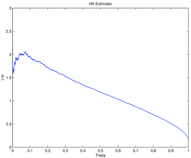
Figure 1: Hill estimator for the tails of $r_{n}$ when $N=10^{3}$, $p=9.5\cdot 10^{-3}$ and $\alpha=0.1$.

Figure 1 is the modified Hill plot (see Apendix C) for $r_{n}$ which numerically confirms these calculations.

2.5 Trend Followers and Value Investors Trading on the Critical Point

To better understand (4), we notice that

$$r_{n+1}=\triangle m_{n+1}+\eta_{n+1}$$

so that the dynamics of the mispricing is

$$\triangle m_{n+1}=-\triangle\alpha\ \triangle m_{n}-\alpha^{tf}\ \triangle m_{n-\theta}-\eta_{n+1}+\alpha^{{}_{tf}}\ \eta_{n}-\alpha^{{}_{tf}}\eta_{n-\theta}$$ (10)

Equation (10)  is a discrete dynamical system with delay structure. By making the substitution

$$(X_{n}^{1},\ldots,X_{n}^{\theta},X_{n}^{\theta+1})\equiv(\triangle m_{n-\theta},\ldots,\triangle m_{n-1},\triangle m_{n})$$ (11)

the dynamics of $\triangle m_{n}$ becomes

$$\mathbf{X}_{n+1}=\mathbf{J}_{m}\mathbf{\ X}_{n}+\mathbf{\eta}_{n}$$ (12)

where $\mathbf{J}_{m}$ is a $(\theta+1)\times(\theta+1)$ companion matrix,

$$\mathbf{J}_{m}=\left[\begin{array}[c]{ccccc}0&1&&&\\ &&1&&\\ &&&\vdots&\\ &&&&1\\ -\alpha^{tf}&0&\ldots&0&-\Delta\alpha\end{array}\right]$$ (13)

and

$$\mathbf{\eta}_{n,\theta}=\left[\begin{array}[c]{l}0\\ \vdots\\ -\eta_{n+1}+\alpha^{{}_{tf}}\ \eta_{n}-\alpha^{{}_{tf}}\ \eta_{n-\theta}\end{array}\right]$$ (14)

If the system has $N_{tf}$ trend followers, equation (13) is time dependent, $\mathbf{J}_{m}\mathbf{\equiv J}_{m}(n)$.

The sum of the capital of active trend followers with time lag $\theta^{(i)}$ at time step $n$ is

$$\alpha_{n}^{tf}(\theta^{(i)})=\sum_{k=1}^{N_{t}}\alpha_{n}^{(k)}\delta_{\theta^{(i)},n}$$

and the difference in capital between (active) value investors and trend followers total capital at time step $n$ is

$$\Delta\alpha_{n}=\sum_{i=1}^{N_{v}}\alpha_{n}^{(i)}\delta_{i,n}-\sum_{j=N_{v}+1}^{N}\alpha_{n}^{(j)}\delta_{j,n}$$

Thus, matrix $\mathbf{J}_{m}(n)$ can be written as:

$$\mathbf{J}_{m}(n)=\left[\begin{array}[c]{ccccc}0&1&0&\ldots&0\\ 0&0&1&\ldots&0\\ &&\vdots&&\\ 0&0&\ldots&0&1\\ -\alpha_{n}^{tf}(\theta^{max})&-\alpha_{n}^{tf}(\theta^{max-1})&\ldots&--\alpha_{n}^{tf}(\theta^{1})&\Delta\alpha_{n}\end{array}\right]$$ (15)

where $\theta^{max}=\max\{\theta^{(i)}\}$ and $\theta^{max-j}=\max\{\theta^{(i)}\backslash\{\theta^{max},\ldots,\theta^{max-j+1}\}\}$. Equation (12) finally becomes:

$$\mathbf{X}_{n+1}=\mathbf{J}_{m}\mathbf{\ }(n)\mathbf{X}_{n}+\mathbf{\eta}_{n}$$ (16)

where

$$\mathbf{\eta}_{n}=\left[\begin{array}[c]{l}0\\ \vdots\\ -\eta_{n+1}+\alpha^{tf}\ \eta_{n}-\sum_{\theta=1}^{\theta_{max}}\alpha_{n}^{tf}(\theta^{i})\ \eta_{n-\theta}\end{array}\right]$$ (17)

Equation (16), together with equation (15) and (17), define an Affine Random Dynamical System (see Apendix A and [3]).

Affine Random Dynamical Systems verify Oseledets’s multiplicative ergodic theorem [3] and thus the Lyapunov numbers are the eigenvalues of

$$\lim_{n\rightarrow\infty}\left[\left(J_{m}^{\ast}\right)^{n}\left(J_{m}\right)^{n}\right]^{1/2n}$$

If the largest Lyapunov exponent of (16) is negative and agents trade w.p. $1$, then (16) is contractive and $\mathbf{\eta}_{n}$ is a stationary process. This means that the mispricing is a random walk and the returns follow a stationary process.

Notice that if $p^{(i)}\neq 1$, $\mathbf{\eta}_{n}$ is not stationary and the mispricing will not follow a random walk, as $\alpha_{n}^{tf}(\theta^{i})$ in (17) will be time dependent. After the results of Section 2.4, an interesting question is ’What is the asymptotic statistics of $r_{n}$ if the traders’ capital and activity probability are chosen so that (4) displays intermittent bursts?’.

For the returns’ correlations to be small, trend followers and value investors should have the same parameters [19]. To simplify the analysis, we will consider that these are trader independent. Thus each trader is characterized by her strategy (value investor/trend follower), her capital, $c$, and her activity probability, $p$. From equation (15), we note that $\left\langle\Delta\alpha_{n}\right\rangle=0$, so that the trend followers’ lag in time provides the oscillations observed on the system. As we vary the traders’ activity probability, $p$, equation (4) approaches the critical point (zero Lyapunov exponent) equation (16) displays on-off intermittent behaviour and the returns’ statistics shows two of the stylized facts of financial time series: fat tails (indexes between $2$ and $4$) and volatility clustering.

The system was simulated for $N_{v}=N_{tf}=5\cdot 10^{3}$, $\lambda=1$, $\theta^{(i)}$ uniformly distributed between $\theta_{min}=1$ and $\theta_{max}=100$, $\eta=0.1$, $c=8\cdot 10^{-2}$ and $p=10^{-2}$. For these parameters, the system is on the critical (non hyperbolic) point of zero Lyapunov exponent and the statistics shown are highly non-trivial. The returns distribution is fat tailed with an index of approximately $3$.

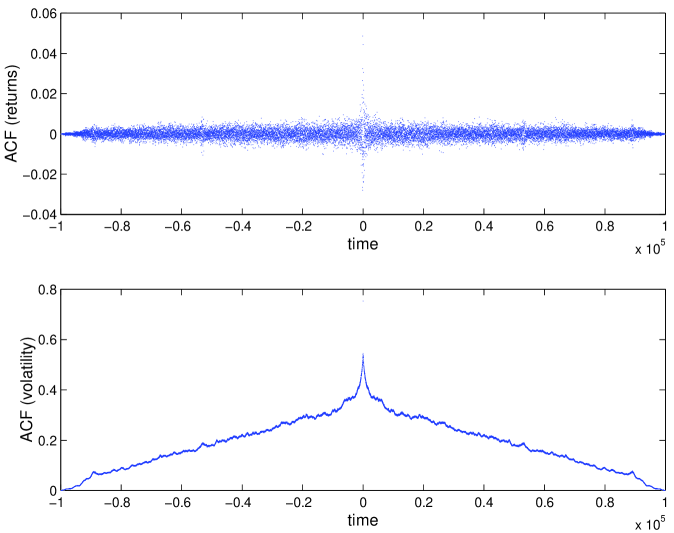
Figure 3: Return and Volatility Autocorrelation Functions for the case in Fig 2.

Nevertheless, it is difficult to infer from Fig. 3 whether the decay of the autocorrelation function is exponential or power law. Let us introduce the generalized correlations $C_{q}\left(\tau\right)$:

$$C_{q}\left(\tau\right)\equiv\left\langle\left|r_{t}\right|^{q}\left|r_{t+\tau}\right|^{q}\right\rangle-\left\langle\left|r_{t}\right|^{q}\right\rangle\left\langle\left|r_{t+\tau}\right|^{q}\right\rangle$$

When the absolute returns series has long memory, $C_{q}\left(\tau\right)$ is a power law:

$$C_{q}\left(\tau\right)\sim\tau^{-\beta_{q}}$$

If $\left|r_{t}\right|^{q}$ is an uncorrelated process one has $\beta_{q}\sim 1$, while $\beta_{q}$ less than $1$ corresponds to long range memory. Let us introduce the generalized cumulative absolute returns [9]

$$\chi_{t,q}\left(\tau\right)\equiv\frac{1}{\tau}\sum_{i=0}^{\tau-1}\left|r_{t+\tau}\right|^{q}$$

and their variance

$$\delta_{q}\left(\tau\right)\equiv\left\langle\chi_{t,q}\left(\tau\right)^{2}\right\rangle-\left\langle\chi_{t,q}\left(\tau\right)\right\rangle^{2}$$

Baviera et al. [9] show that if $C_{q}\left(\tau\right)$ for large $\tau$ is a power-law with exponent $\beta_{q}$, then $\delta_{q}\left(\tau\right)$ is a power-law with the same exponent. That is

$$C_{q}\left(\tau\right)\sim\tau^{-\beta_{q}}\Longrightarrow\delta_{q}\left(\tau\right)\sim\tau^{-\beta_{q}}$$

In other words, the hypothesis of long range memory for the absolute returns can be checked via the numerical analysis of the variance of the absolute cumulative returns.

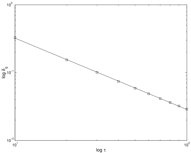
Figure 4: Volatility of cumulative absolute returns.

In Fig 4 we plot the volatility of the absolute cumulative returns. We determine an exponent $\beta_{1}\simeq 1$, thus concluding that the autocorrelation function has an exponential decay, contrary to the stylized facts presented on page 1. We speculate that this is due to the intrinsic linearity of the model.

3 Discussion

We have shown that when the dominant strategy is value investing, if there exist $N,\alpha,$ $p$ and $\mu\in\left[k,k+1\right]$ that satisfy (26) then

$$Prob\left(\left|r_{n}\right|>x\right)\approx c\cdot x^{-\mu}$$ (18)

and the returns display a probability distribution asymptotic to a power tail of exponent $\mu$. We have also shown that, if one fixes $N$ and $p$, one can determine heuristically $\alpha$ such that the probability distribution of $r_{n}$ is given by (18) with the desired $\mu$.

The association of an unconditional trading probability to each agent, permits intermittent bursts on market price and a fat tailed distribution for the returns. This is, to our knowledge, the first model that discusses fat tail distributions caused by value investor strategies only.

We have shown that when trend followers and value investors are together on the market trading at each time step, the mispricing is a random walk, independently of the maximum lag in time, $\theta^{max}$ of the trend followers. Trend followers do not seem to introduce relevant correlations on the returns. A mixture of negative short-term dependence (the value investors) with long-term positive dependence (the trend followers) obscures the underlying dependence structure leading to apparent insignificant correlations [19].

When the system is near the critical point (zero Lyapunov exponent) and each trader has a relatively high capital and a low trading probability, the system displays on-off intermittency. Further, the returns’ distribution is fat tailed and volatility is clustered.

We see our model as a first step towards an explanation of the stylized facts of finance in the framework of a semi-analytical random dynamical system. The feedback present in the model leads to volatility clustering, but is yet to be improved so that the volatility autocorrelation function has a power-law decay.

Whether the present work is relevant and lessons for the market can be drawn from it depends on the reliability of simulated price and return time series (where it is noted that no mechanism provides any cointegration between price and fundamental value) and on the acceptance of the underlying model [19].

4 Appendix A

A random dynamical system (RDS) has two ingredients; $(i)$ a model of the noise in the form of a measure-preserving transformation and $(ii)$ a model of the deterministic dynamics consisting of a family of continuous transformations. Which transformation is applied depends on the state of the noise at that moment in time. We examine RDS generated by iterating skew product maps of the form[5, 6]

$$\omega(t) =\theta_{t}\omega$$

$$y\left(t\right) =\phi\left(t,\omega\right)y$$

where $\theta_{t}$ is a flow and $\phi\left(t,\omega\right)$ is a cocycle (i.e. is such that $\phi(t+s,\omega)=\phi(t,\theta_{s}\omega)\circ\phi\left(s,\omega\right)$ for all $t,s>0$). $\omega$ represents the state of a dynamical system that models the noise process and $y$ represents the dynamical system forced by the noise. We write $\theta_{t}\omega$ (resp. $\phi\left(t,\omega\right)y$) to mean a nonlinear map $\theta_{t}$ (resp. $\phi\left(t,\omega\right)$) applied to the point $\omega$ (resp. $y$). In particular, the action of $\theta$ and $\phi$ need not be linear. In the case that the evolution is chaotic we can see the above system as random forcing of a deterministic system $\phi$ where the evolution of $\omega$ is ‘hidden’. By looking at such systems one can get a more detailed picture of the dependence of a dynamical system on noise than is possible by, for example, a Fokker-Planck approach.

We assume that the evolution $\theta$ has an ergodic invariant probability measure $\mathcal{P}$ with respect to which an initial condition for $\omega$ is chosen from a set of full measure. Random dynamical systems studies the dynamics of the full system relative to the dynamics of the measure-preserving transformation $(\theta,P)$ ( $\mu$ is defined on subsets in some $\sigma$-algebra).

A random dynamical system is said to be affine if

$$\phi\left(t,\omega\right)y=\Phi\left(t,\omega\right)y+\psi\left(t,\omega\right)$$

where $\Phi\left(t,\omega\right)$ is a linear cocycle and

$$\psi\left(t+s,\omega\right)=\Phi\left(t,\theta_{s}\omega\right)\psi\left(s,\omega\right)+\psi\left(t,\theta_{s}\omega\right),\qquad t,s\geq 0$$

5 Appendix B

Proof of Lemma 1: The kth moment of $\alpha_{n}^{\mu}$ is given by

$$M^{(k)}(0)=\sum_{i=0}^{N}i^{k}p^{i}(1-p)^{N-i}\left(\begin{array}[c]{l}N\\ i\end{array}\right)$$ (19)

A Taylor series expansion of (19) in $p$ to second order about the origin yields

$$M^{(k)}(0)=\left\{\begin{array}[c]{ll}\qquad Np&k=1\\ Np\left[1+(2^{k-1}-1)(N-1)p\right]+O^{3}(p)&k\geq 2\end{array}\right.$$

So that

$$\begin{array}[c]{lll}\left(\frac{M^{(k+1)}(0)}{M^{(k)}(0)}\right)^{k}&=&\left(\frac{1+(2^{k}-1)(N-1)p}{1+(2^{k-1}-1)(N-1)p}\right)^{k}\\ &=&\left(1+\frac{2^{k-1}(N-1)p}{1+(2^{k-1}-1)(N-1)p}\right)^{k}\end{array}$$ (20)

We want to prove that for $p$ small enough

$$\left(\frac{M^{(k+1)}(0)}{M^{(k)}(0)}\right)^{k}>M^{(k)}(0)$$

Which is equivalent to

$$\left(1+\frac{2^{k-1}(N-1)p}{1+(2^{k-1}-1)(N-1)p}\right)^{k}>\left(1+(2^{k-1}-1)(N-1)p\right)Np$$ (21)

Expanding both sides in a Taylor series in $p$ about the origin, we obtain the relation

$$1+2^{k-1}k(N-1)p+O^{2}(p)>Np+O^{2}(p)$$

which, to first order in $p$, is equivalent to

$$N>\frac{2^{k-1}k}{2^{k-1}k-1}-\frac{1}{\left(2^{k-1}k-1\right)p}$$

which is valid for $k>1$ and $N>1$.$\blacksquare$

Proof of Lemma 2:

The solution of (6) is given by [25]

$$r_{n}=\sum_{k=1}^{n}\left(\prod_{j=k+1}^{n}-\alpha_{j}\right)\alpha_{k}\eta_{k}+\left(\prod_{j=1}^{n}-\alpha_{j}\right)r_{0}$$

where $\prod_{j=n+1}^{n}-\alpha_{j}=1$. The Lyapunov number of (6) is given by

$$\left\langle\alpha_{n}\right\rangle=\alpha M^{(1)}(0)=\alpha Np$$ (22)

If $\left\langle\alpha_{n}\right\rangle<1$ (negative Lyapunov exponent)

$$\prod_{j=1}^{n}-\alpha_{j}^{vi}\underset{n\rightarrow\infty}{\rightarrow}0$$

exponentially fast and under very weak conditions on the product $\alpha_{k}\eta_{k}$, the distribution of $r_{n}$ will converge independently of $r_{0}$ to that of the series

$$\sum_{k=1}^{n}\left(\prod_{j=k+1}^{n}-\alpha_{j}\right)\alpha_{k}\eta_{k}$$ (23)

Thus, if $\alpha<\frac{1}{M^{(1)}(0)}$, $r_{n}$ converges in distribution to a unique limiting distribution, that of (23). As the binomial moments $M^{(k)}(0)$ are increasing functions of $k$ this condition is satisfied for $\alpha\in I_{k,k+1}\quad\forall k\in\mathbb{N}$.$\mathbb{\blacksquare}$

As can be observed from (23), the additive term in (6), $\alpha_{n}\eta_{n}$, provides a reinjection mechanism, allowing $r_{n}$ to fluctuate without converging to zero, as it would if $\alpha_{n}\eta_{n}$ vanished [37].

Proof of Proposition 1: If the agents’ normalized capitals and trading probabilities are constants, respectively $\alpha_{n}^{(i)}=\alpha$ and $p^{(i)}=p$,

$$\left\langle\left(\alpha_{n}^{vi}\right)^{\mu}\right\rangle=\alpha^{\mu}\sum_{i=0}^{N}i^{\mu}\,\,p^{i}(1-p)^{N-i}\binom{N}{i}$$ (24)

Theorem 1 requires the existence of a $\mu>0$ such that

$$\left\langle\left(\alpha_{n}^{vi}\right)^{\mu}\right\rangle=1$$ (25)

Although the estimation of $\mu$ from (25) is in general not possible, one can estimate an interval for $\mu$. Choose $p\in\left]0,1\right[$ and $\{N,k\}\in\mathbb{N}^{2}$. As the binomial moments $M^{(k)}(0)$ are continuous and increasing functions of $k$, equation (25) is satisfied if there exists an $\alpha$ such that

$$\left\{\begin{array}[c]{c}\left\langle\left(\alpha_{n}^{vi}\right)^{k}\right\rangle=\alpha^{k}M^{(k)}(0)<1\\ \left\langle\left(\alpha_{n}^{vi}\right)^{k+1}\right\rangle\alpha^{k+1}M^{(k+1)}(0)>1\end{array}\right.$$ (26)

From (24) and (26), one deduces that $\alpha\in I_{k,k+1}$.$\blacksquare$

6 Appendix C

Suppose $\left\{X_{n},n\geq 1\right\}$ is a stationary sequence and that

$$P\left[X_{1}>x\right]=x^{-\alpha}L\left(x\right),\qquad x\rightarrow\infty$$

where $L$ is slowly varying and $\alpha>0$. Let

$$X_{\left(1\right)}>X_{\left(2\right)}>\cdots>X_{\left(n\right)}$$

be the order statistics of the sample $X_{1},\cdots,X_{n}$. We pick $k<n$ and define the Hill estimator to be [1]

$$H_{k,n}=\frac{1}{k}\sum_{i=1}^{k}\log\frac{X_{\left(i\right)}}{X_{\left(k+1\right)}}$$

where $k$ is the number of upper order statistics used in the estimation. The Hill plot is the plot of

$$\left(\left(k,H_{k,n}^{-1}\right),1\leq k<n\right)$$

and, if the processs is linear or satistifies mixing conditions, then since $H_{k,n}\overset{P}{\rightarrow}\alpha^{-1}$ as $n\rightarrow\infty$, $k/n\rightarrow 0$ the Hill plot should have a stable regime sitting at height roughly $\alpha$.

As an alternative to the Hill plot, it is sometimes useful to display the information provided by the Hill estimation as [18]

$$\left\{\left(\theta,H_{\left\lceil n^{\theta}\right\rceil,n}^{-1}\right),0\leq\theta\leq 1\right\},$$

where we write $\left\lceil y\right\rceil$ for the smallest integer greater or equal to $y\geq 0$. We call such plots the alternative Hill plot. The alternative display is sometimes revealing since the original order statistics get shown more clearly and cover a bigger portion of the displayed space.

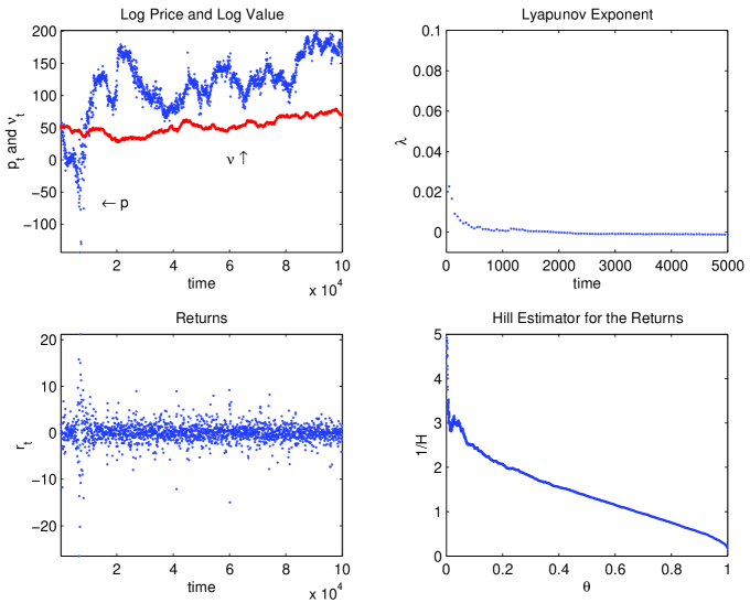
Figure 2: Simulation with $N_{v}=N_{tf}=5\cdot 10^{3}$, $\lambda=1$, $\eta=0.1$, $\theta_{min}=1$ and $\theta_{max}=100$, $c=8\cdot 10^{-2}$ and $p=10^{-2}$.

References

- [1] Adler, Robert J., et al. A Practical Guide to Heavy Tails. Birkhauser, 1998.
- [2] Arifovic, Jasmina and Ramazan Gençay. “Statistical properties of genetic learning in a model of exchange rate,” J. Econ. Dynam. Control, 24:981–1005 (2000).
- [3] Arnold, Ludwig. Random Dynamical Systems. Springer-Verlag, 1998.
- [4] Arthur, W. Brian, et al. “Asset Pricing Under Endogenous Expectations in an Artificial Stock Market.” The Economy as an Evolving, Complex System II Addison-Wesley, 1997.
- [5] Ashwin, Peter. “Attractors of a randomly forced electronic oscillator,” Phys. D, 125:302–310 (1999).
- [6] Ashwin, Peter. “Minimal attractors and bifurcations of random dynamical systems,” Proc. Roy. Soc. London A, 455:2615–2634 (1999).
- [7] Bak, Per, et al. “Self-organized criticality,” Physical Review A, 38:364 374 (1987).
- [8] Bak, Peter, et al. “Aggregate Fluctuations from Independent Sectoral Shocks: Self-Organized Criticality in a Model of Production and Inventory Dynamics,” Ricerche Economiche, 47:3–30 (1993).
- [9] Baviera, Roberto, et al., “Efficiency in foreign exchange markets,” 2001.
- [10] Beja, A. and M. B. Goldman. “On the Dynamic Behavior of Prices in Disequilibrium,” J. Finance, 35:235 – 248 (1980).
- [11] Boffetta, G., et al., “Predictability: a way to characterize Complexity,” 2001. available at http://xxx.lanl.gov/abs/nlin.CD/0101029.
- [12] Bouchaud, Jean-Philippe and Rama Cont. “A Langevin approach to stock market fluctuations and crashes,” Euro. Phys. J. B, 6:543–550 (1998).
- [13] Brock, William A. and Patrick de Fontnouvelle. “Expectational diversity in monetary economies,” J. Econ. Dynam. Control, 24:725–759 (2000).
- [14] Brock, William A. and Cars H. Hommes. “Heterogeneous beliefs and routes to chaos in a simple asset pricing model,” J. Econ. Dynam. Control, 22:1235–1274 (1998).
- [15] Cabrales, Antonio and Takeo Hoshi. “Heterogeneous beleifs, wealth accumulation, and asset price dynamics,” J. Econ. Dynam. Control, 20:1073–1100 (1996).
- [16] Chiarella, Carl. “The Dynamics of Speculative Behaviour,” Ann. Oper. Res., 37:101–123 (1992).
- [17] Day, R. H. and W. Huang. “Bulls, Bears and Market Sheep,” J. Econ. Behav. Organ., 14:299 – 329 (1990).
- [18] Dress, Holger, et al., “How to make a Hill plot,” 1999. Available at http://www.orie. cornell.edu/trlist/trlist.html.
- [19] Farmer, J. Doyne. “Market force, ecology, and evolution,” Santa Fe Institute Working Paper 98-12-117 (1998).
- [20] Farmer, J. Doyne and Shareen Joshi. “The price dynamics of common trading strategies,” J. Econ. Behav. Organ. (2001). To appear.
- [21] Feller, W. An Introduction to Probability Theory and Its Applications, 2. New York: John Wiley & Sons, 1971.
- [22] Gaunersdorfer, Andrea and Cars H. Hommes. A Nonlinear Structural Model for Volatility Clustering. Technical Report CeNDEF Working paper 00-01, University of Amsterdam (2000), August 2000 2000.
- [23] Gaunersdorfer, Andrea, et al. Bifurcation Routes to Volatility Clustering. Technical Report Working Paper 73, Vienna University of Economics and Business Administration, September 2000.
- [24] Gopikrishnan, P., et al. “Inverse Cubic Law for the Distribution of Stock Price Variations,” Eur. Phys. J. B, 3:139–140 (1998).
- [25] Haan, Laurens de, et al. “Extremal Behaviour of Solutions to a Stochastic Difference Equation with Applications to ARCH Processes,” Stochastic Process. Appl., 32:213–224 (1989).
- [26] Heagy, J.F., et al. “Characterization of on-off intermittency,” Phys. Rev. E, 49(2):1140–1150 (1994).
- [27] Iori, Giulia. “A microsimulation of traders activity in the stock market: the role of heterogeneity, agents’ interactions and trade frictions,” J. Econ. Behav. Organ. (2001). in press.
- [28] Kesten, Harry. “Random Difference Equations and Renewal Theory for Products of Random Matrices,” Acta Math., (131):207–248 (1973).
- [29] Lux, Thomas. “Herd Behaviour, Bubbles and Crashes,” Econ. J., 105:881–896 (1995).
- [30] Lux, Thomas. “The socio-economic dynamics of speculative markets: interacting agents, chaos, and the fat tails of return distributions,” J. Econ. Behav. Organ., 33:143–165 (1998).
- [31] Lux, Thomas and Michele Marchesi. Volatility Clustering in Financial Markets: A Microsimulation of Interacting Agents. Technical Report B-437, Bonn University, July 1998.
- [32] Lux, Thomas and Michele Marchesi. “Scaling and Criticality in a Stochastic Multi-Agent Model of a Financial Market,” Nature, 397:498 – 500 (1999).
- [33] Platt, N., et al. “On-Off Intermittency: A Mechanism for Bursting,” Phys. Rev. Lett., 70(3):279–282 (1993).
- [34] Rim, Sunghwan, et al. “Chaotic Transition of Random Dynamical Systems and Chaos Synchronization by Common Noises,” Phys. Rev. Lett., 85(11):2304–2307 (2000).
- [35] Sarno, Lucio and Mark P. Taylor. “Moral hazard, asset price bubbles, capital flows, and the East Asian crisis: the first tests,” J. Int. Money Finance, 18:637 (1999).
- [36] Sethi, R. “Endogenous regime switching in speculative markets,” Struct. Change Econ. Dynam., 7:99–118 (1996).
- [37] Sornette, Didier and Rama Cont. “Convergent Multiplicative Processes Repelled from Zero: Power Laws and Truncated Power Laws,” J. Phys. I, 7:431–444 (1997).