[

Structural glass on a lattice in the limit of infinite dimensions.

Abstract

We construct a mean field theory for the lattice model of a structural glass and solve it using the replica method and one step replica symmetry breaking ansatz; this theory becomes exact in the limit of infinite dimensions. Analyzing stability of this solution we conclude that the metastable states remain uncorrelated in a finite temperature range below the transition, but become correlated at sufficiently low temperature. We find dynamic and thermodynamic transition temperatures as functions of the density and construct a full thermodynamic description of a typical physical process in which the system gets trapped in one metastable state when cooled below vitrification temperature. We find that for such physical process the entropy and pressure at the glass transition are continuous across the transition while their temperature derivatives have jumps.

]

Thermodynamics of structural glasses and of vitrification transition is a long standing problem in statistical physics. The essential feature of glass formation is a division of the phase space into an exponentially large number of similar compartments. The system gets trapped in one of these compartments and stays there forever in a complete defiance of ergodic hypothesis; this defines dynamical ”states” of the system. Each of these states is characterized by a local order parameter (e.g. atoms positions, magnetization) that varies in space and distinguishes one state from another. This makes even a mean field theory difficult to construct because the thermodynamic ground state of the system (or any other particular state) has a unique configuration of the order parameter field, thus making it difficult to describe system in terms of average (and site independent) quantities. Few ways to resolve this difficulty were proposed recently [2, 3, 4, 5, 6, 7, 8]; they all share a common idea that states of the system with the same energy per site (but perhaps different total energies) are essentially equivalent and instead of studying one particular state one can average over all states with the same energy density.

There are a few ways to implement averaging over states, the most convenient ones seem to be the clone method [6, 7] and the introduction of a small random field conjugated to the order parameter (magnetization in case of spin glasses or density in structural glasses) [8]. The physical idea of the latter is that an infinitesimally small random field applied to a system with many metastable states rearranges the energies of low-lying states making the problem similar to one with quenched disorder. In a spin system, for example, we add to the Hamiltonian a magnetic field part: ${\cal H}\rightarrow{\cal H}+\sum_{i}h_{i}S_{i}$ with small random $h_{i}$. The resulting change in the energy of a typical metastable state is of the order of $\sqrt{N}h$; because this energy interval contains a large number of metastable states, we expect that a small non-zero field would result in a large rearrangement of their energies but would not change the properties of individual states. Averaging over the random field configurations may be then performed in a usual way introducing $n$ replicas of the system and taking the limit $n\rightarrow 0$. The alternative idea of the clone method is to consider a system of $m$ clones constrained to be in the same metastable states by an infinitesimally weak coupling. Generally, the free energy density of the clone system may be written as $F_{clone}=-TN^{-1}\ln\int dFe^{-N(m\beta F-S_{conf}(F))}$ where $S_{conf}(F)$ is configurational entropy ($S_{conf}=\frac{1}{N}\ln({\cal N}_{states})$). If $S_{conf}(F)$ is concave and $dS_{conf}(F)/dF$ is finite at the lower bound $F=F_{0}$ (corresponding to the ground state) the appropriate choice of $m$ ($m\propto T$ at low $T$) leads to a partition function dominated by a small vicinity of any given $F>F_{0}$ that still contains thermodynamic number of states providing the averaging mechanism in this approach. In this paper we shall apply the mean field formalism developed in our paper [8] that combines random field approach and the locator expansion developed for the glass physics in [10] to the simplest model of a realistic structural glass. The mean field theory for the structural glasses can be justified formally only in the limit of infinite dimensions; thus, in our derivation of the mean field theory below we shall consider the space of arbitrary dimension, $d$, and keep only the leading terms in $1/d$. We hope, however, that it provides reasonable results even for $d=3$ because the actual parameter is the coordination number which is already large in three dimensions.

Another important physical assumption that simplifies the calculations significantly is that different states are uncorrelated. Formally, this allows one to look for one step replica symmetry breaking (RSB) solution of the mean field equations. We check the stability of this solution below and find that it is stable in some temperature range below the glass transition temperature but that it becomes unstable at low temperatures. The results of one step RSB can be translated much easier into the physical properties than results of a full RSB because in this case one can establish a formal equivalence between this method and a clone approach with the number of clones being equal to the size of the blocks in 1RSB ansatz $m,$ and replica free energy $F_{repl\text{ }}$ being equal to the free energy of the clone system per one clone $F_{repl}=F_{clone}/m.$ For a given $m$ the main contribution to $F_{clone}$ comes from states with $m=TdS_{conf}(F)/dF$ , thus

$$S_{conf}=\beta m^{2}\frac{\partial}{\partial m}(F_{clone}/m),\,\,\,F=\frac{\partial}{\partial m}F_{clone.}$$ (1)

Metastable states first appear at the dynamical transition temperature $T_{g},$ at which the system becomes trapped in one of the metastable states with largest possible free energy $F$ because these states dominate the configuration space since $S_{conf}(F)$ is a monotonically increasing function. Under a further decrease of temperature the system remains trapped in the same metastable state, thus the thermodynamics of a physical cooling process is determined by the free energy of a single metastable state. To describe this physical process by a replica method we need to find the dependence $m(T)$ consistent with the requirement that the physical system is trapped in a single metastable state. We assume that all states that were similar at one temperature remain similar as the temperature is decreased and these states do not bifurcate or disappear (consistent with one step RSB); this implies that configuration entropy $S_{conf}$ is constant along the trajectory $m(T)$ corresponding to a physical cooling process. We check that this assumption is consistent with (1) that gives the free energy of a metastable state and the corresponding configuration entropy in terms of the replica free energy. First, we note that the usual thermodynamic identity $E=\partial[\beta F_{repl}(\beta,m)]/\partial\beta$ that relates internal energy to the free energy remains valid in replica approach. Second, if the system is trapped in a single metastable state, the thermodynamic identity $E(\beta,m)=d[\beta F(\beta,m)]/d\beta$ must also hold. Remarkably, these equations are consistent with each other and with (1) if and only if $S_{conf}(\beta,m)=const$. This gives us the implicit equation for $m(T)$ and allows us to deduce the thermodynamics of the system trapped in a single metastable state provided  one step RSB is a stable solution.

We now turn to the details of the model and its solution. We consider the simplest glass model which contains only short range repulsion between atoms:

$$H={\frac{1}{2}}\sum_{i.j}\rho_{i}J_{i,j}\rho_{j}$$ (2)

where $i,j$ are the sites of a d-dimensional lattice and $\rho_{i}=1,0$ represents the on-site density. The glass is formed for such coupling matrices $J_{i,j}$ that do not allow low energy crystal states (density waves). It is convenient to represent $J_{i,j}$ in the form $\hat{J}=uf(\hat{t}/\sqrt{2d}),$ where $\hat{t}$ is the nearest neighbor hopping operator and we introduced the scaling $\sqrt{2d}$ that is needed to get a sensible limit at $d\rightarrow\infty\cite[cite]{[\@@bibref{Number}{Georges}{}{}]}.$ The simplest choice of the function $f(\varepsilon)\sim\varepsilon$ leads to the crystal ground state with a chess-board ordering for density $\bar{\rho}\approx 1/2.$ We shall take $f(\varepsilon)=\varepsilon^{2}$ and show that this frustrated interaction leads to the formation of the glass state at low temperature.

The Hamiltonian (2) may be represented as $H=H_{0}+H^{\prime},$ separating out large but physically irrelevant constant term $H_{0}=ud\bar{\rho}^{2}$. We focus on the nontrivial term $H^{\prime}=\sum_{i,.j}\tilde{\rho}_{i}J_{i,j}\tilde{\rho}_{j}$ where $\tilde{\rho}=\rho-\bar{\rho}.$ Introducing the replicas we get

$$\beta H^{\prime}=\frac{\beta}{2}\sum_{i,j,\alpha}\tilde{\rho}_{i}^{\alpha}J_{i,j}\tilde{\rho}_{j}^{\alpha}-\sum_{i,\alpha}\mu^{\alpha}\tilde{\rho}_{i}^{\alpha}$$ (3)

where $\alpha$ is the replica index taking values form $0$ to $n,$ and $\mu_{\alpha}$ are the the Lagrange multipliers (equal to the chemical potential divided by the temperature at the saddle point) that impose constraint on the number of particles in each replica. In the limit of infinite dimensions the original model (3) can be replaced with an effective single site model

$$-\beta H_{eff}^{\prime}=\frac{1}{2}U({\cal B})-\frac{1}{2}\tilde{\rho}_{\alpha}B_{\alpha,\beta}\tilde{\rho}_{\beta}+\mu_{\alpha}\tilde{\rho}_{\alpha}$$ (4)

where ${\cal B}$ is the matrix in replica space and $\tilde{\rho}=\rho-\bar{\rho}$ has only replica index. The mean field self-consistency condition is that $B$ gives the saddle point of the free energy: $\langle\tilde{\rho}_{\alpha}\tilde{\rho}_{\beta}\rangle=dU({\cal B})/dB_{\alpha\beta}$. The potential $U({\cal B})$ can be determined from the condition that all single site correlation functions of the model (4) coincide with the correlation functions of the original model (3). Instead of comparing these correlation functions directly we decouple the interaction term introducing the auxiliary fields, $v^{\alpha}$, conjugated to $\tilde{\rho}$

$$-\beta H^{\prime}= - \frac{T}{2}\sum_{i,j,\alpha}v_{i}^{\alpha}J_{i,j}^{-1}v_{j}^{\alpha}+\sum_{i,\alpha}\tilde{\rho}_{i}^{\alpha}(iv_{i}^{\alpha}+\mu^{\alpha})$$ (5)

$$- \frac{n}{2}{\rm Tr}\log\hat{J}\beta$$ (6)

$$-\beta H_{eff}^{\prime}= - \frac{1}{2}\sum_{\alpha,\beta}v^{\alpha}B_{\alpha,\beta}^{-1}v^{\beta}+\sum_{\alpha}\tilde{\rho}^{\alpha}(iv^{\alpha}+\mu^{\alpha})$$ (7)

$$+ \frac{1}{2}U(B)-\frac{1}{2}{\rm Tr}\log B$$ (8)

and compare the correlation functions of these fields. Summation over $\tilde{\rho}$ in both models results in the on-site interaction of the fields $v.$ Inspecting the terms of the perturbation theory in this on-site interaction for the correlator $G_{i,j}^{\alpha\beta}=\langle v_{i}^{\alpha}v_{j}^{\beta}\rangle$ one verifies that in the leading order in $1/d$ it is given by $\hat{G}=[T\hat{J}^{-1}-\Sigma]^{-1}$ with the self energy $\Sigma$ which is diagonal in the site index: $\Sigma=-({\cal A}\,\beta u)^{-1}\delta_{ij}$. This approach is similar to a locator expansion [10] but in our case the locator ${\cal A}$ is non-trivial in the replica space. The single site correlation function ${\cal G}_{\alpha\beta}\equiv G_{i,i}^{\alpha\beta}$ (that we need to establish the correspondence between the models) is

$${\cal G}=u\beta\int d\epsilon\nu(\epsilon)[1/f(\varepsilon)+{\cal A}^{-1}]^{-1}$$ (9)

where $\nu(\varepsilon)=\exp[-\varepsilon^{2}/2]/\sqrt{2\pi}$ is the density of states in the limit $d\rightarrow\infty.$

Now we turn to the model (8). Here the self energy is diagonal in the site index by construction, further, the interaction part of this model is the same as for model (6); assuming that their single site correlation functions coincide, we get that their single site self-energies are equal, so that for this model

$${\cal G}=[{\cal B}^{-1}+(\beta u{\cal A)}^{-1}]^{-1}$$ (10)

which gives us equation relating ${\cal B}$ and ${\cal A}$. Further, the correlation function of the auxiliary fields can be expressed through ${\cal D}=\langle\tilde{\rho}_{\alpha}\tilde{\rho}_{\beta}\rangle$ via ${\cal G=B-B}{\cal D}{\cal B}$, combining this equation with the saddle point condition and using $\int d\varepsilon D(\varepsilon)=1$ we find the implicit expression for the potential

$\displaystyle U(B)={\rm Tr}\ln[{\cal A}+{\cal B}/u\beta]-{\rm Tr}\int d\epsilon D(\epsilon)\ln({\cal A}+f(\varepsilon))$

that has to be evaluated at the saddle point with respect to ${\cal A}.$

Liquid state. In the liquid phase we take the replica symmetric ansatz $A_{\alpha,\beta}=a\delta_{\alpha,\beta},B=b\delta_{\alpha,\beta}$, exclude the chemical potential $\mu$ and get

$$\beta F=[L(a)-\ln(a+b/u\beta)+b\bar{\rho}(1-\bar{\rho})]/2-S_{0},$$ (11)

where $L(a)=\int d\varepsilon\nu(\varepsilon)\ln(a+\varepsilon^{2})$ and $S_{0}=-\bar{\rho}\ln\bar{\rho}-(1-\bar{\rho})\ln(1-\bar{\rho})$ is the high temperature entropy. The corresponding energy is $E=T\bar{\rho}(1-\bar{\rho})b/2.$ Numerical solution of the saddle point equations show that at any density the entropy becomes negative at low temperatures. The dependence of the temperature at which the entropy becomes zero $T_{S=0}$ on the density for the coupling constant $u=1$ is shown in Fig. 1. This line provides the lower bound for the glass transition temperature.

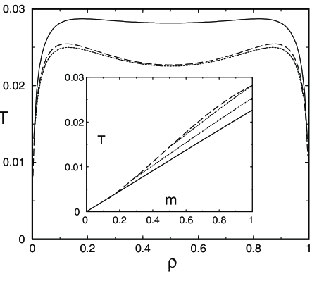
FIG. 1.: Dynamical (solid line) and thermodynamical (dashed line) transition temperatures as functions of density. The dotted line shows the temperature at which the entropy of the liquid state becomes negative. The insert shows the trajectory $T(m)$ for thermodynamic (solid line) and marginal (dashed line) solutions. The dotted lines represent the trajectories with constant configuration entropy: The upper one ($S_{conf}=0.07286$) corresponds to the physical cooling process in which the system is trapped at the dynamical transition temperature. The lower one ($S_{conf}=0.04$) represents a process when a system trapped in a lower energy state.

Glass state. In the glass phase the replica symmetry is broken, we assume that the solution has one step RSB structure and then verify that it is indeed a stable solution. Taking $B_{\alpha,\beta}=b_{1}\delta_{\alpha,\beta}-b_{2}\,R_{\alpha,\beta},A_{\alpha,\beta}=a_{1}\delta_{\alpha,\beta}-a_{2}\,R_{\alpha,\beta}$ where the matrix $R$ is a block-diagonal matrix consisting of $m\times m$ blocks with all elements equal $1$, we get the free energy functional

$$\beta F_{repl} = \frac{m-1}{2m}[L(a_{1})-\ln(a_{1}+\frac{b_{1}}{u\beta})]+\frac{L(a_{1}-ma_{2})}{2m}$$ (12)

$$- \frac{1}{2m}\ln X-\frac{1}{m}\ln Z_{m}+\mu\bar{\rho}+\frac{1}{2}\bar{\rho}^{2}(b_{1}-mb_{2})$$ (13)

where $X=a_{1}-ma+(b_{1}-mb_{2})/u\beta$ and

$\displaystyle Z_{m}=\int P_{m}(y)dy,P_{m}(y)=e^{-y^{2}/2}(1+e^{h+y\sqrt{b_{2}}})^{m}/\sqrt{2\pi},$

with $h=\mu+\bar{\rho}(b_{1}-mb_{2})-b_{1}/2.$ The free energy (13) has to be taken at the saddle point with respect to $a_{1},a_{2},b_{1},b_{2}.$ For the thermodynamic solution it should be also at the saddle point with respect to $m,$ according to (1) it means that $S_{conf}=0.$ The numerical solution for the dependence of temperature on $m$ at fixed density ($\bar{\rho}=0.5$) is shown in Fig 1 insert. By definition $0<m<1,$ thus the value of temperature for which $m=1$ determines the thermodynamic glass transition temperature $T_{c}.$ It is plotted as a function of density in Fig. 1.

Stability and marginal solution. In order to analyze stability of one step RSB ansatz we expand the Eq.(4) to the second order in fluctuation of the order parameter $\delta B$ and consider different families of fluctuation matrices $\delta B$. This calculation is very similar to the analysis of the stability of paramagnetic solution and Parisi solution in SK model [12, 13] so we only sketch it here. We find that the most dangerous direction in the fluctuation space corresponds to the ”replicon” modes [12, 13] that are fluctuations within diagonal blocks of $\delta B$ satisfying the conditions $(\delta B\,R)_{\alpha,\beta}=0$, $\delta B_{\alpha,\alpha}=0.$ The eigenvalue corresponding to these modes is

$\displaystyle\Lambda=\frac{2}{(u\beta)^{2}\chi^{-1}(a_{1})-(\bar{\rho}-g_{2})^{-2}}+2(g_{2}-2g_{3}+g_{4})$

where $g_{k}=\int P_{m}(z)[1+\exp(-h-z\sqrt{b_{2}})]^{-k}dz/Z_{m}$ and $\chi(a)=\int\exp[-\varepsilon^{2}/2](a+\varepsilon^{2})^{-2}dx/\sqrt{2\pi}.$ Numerical solution shows that for any density the thermodynamic solution is stable in the wide temperature range below $T_{c}$ but eventually becomes unstable at low temperature. The solution corresponding to marginally stable states is obtained by taking $\Lambda=0,$ the corresponding $T(m)$ dependence is plotted in Fig. 1 insert. As was explained above $m=1$ defines the dynamical glass transition temperature $T_{g}$, which is plotted as a function of density in Fig. 1.

Physical cooling. During the physical cooling process the system remains trapped in a single metastable state. As was explained above, the physical properties of such system are described by the trajectory $m(T)$ satisfying $S_{conf}(m,T)=const$. We show two such trajectories in the insert of Fig. 1. The upper dotted line correspond to a typical process in which the system got trapped in the highest energy state at the dynamical transition temperature (for this curve $S_{conf}=0.072864$), the lower one to a system trapped in a lower energy state corresponding to $S_{conf}=0.04$. We see that these trajectories cross the marginal stability line at lower temperatures, beyond this line the one step RSB ansatz becomes unstable. Physically, it means that a metastable state in which the system is trapped starts to divide into new ones.

Thermodynamics of the glass transition. General thermodynamic arguments show that static properties (specific heat, pressure) of the glass transition are controlled by the total entropy $S_{tot}=S+S_{conf}$. We show the temperature dependence of $S_{tot}$ and entropy of the liquid state for density $\bar{\rho}=1/2$ in Fig 2. The upper dotted line represents the physical cooling that begins from the dynamical glass transition temperature $T_{g}.$ We see that the entropy has no jump at the phase transition while its derivative (specific heat) does. We also consider the pressure defined, as usually, by $P=-\partial F/\partial V.$ Along the physical process $S_{conf}=const,$ therefore $P=-\partial F_{rep}/\partial V.$ The corresponding plots are shown in Fig. 2. As in case with the entropy, the pressure has no jump at the phase transition, while its derivative $dP/dT$ does.

In conclusion, we formulated a simple model of the structural glass and solved it in the limit of $d\rightarrow\infty$ using the mean field theory. We constructed a full thermodynamic description of the physical cooling process in which the system is trapped in a single metastable state. At very low temperature a metastable state in which the system is trapped starts to divide into new states, below this temperature our method based on one step RSB ansatz can not be applied. From our analysis we conclude that in this system there is no jump in the entropy or pressure at the glass transition temperature while there are jumps in their temperature derivatives. These qualitative conclusions are in agreement with an established phenomenological picture of the glass transition [14].

FIG. 2.: Temperature dependence of the entropy and pressure in the glass phase (solid and dotted lines) and in the liquid phase (dashed lines). Solid lines correspond to the thermodynamic solution ($S_{conf}=0$), the upper dotted lines represent the total entropy $S_{tot}$ and pressure of the physical cooling process ($S_{conf}=0.072864$) in which the system is trapped at the dynamical transition temperature, the lower dotted lines correspond to a process when a system trapped in a lower energy state (corresponding to $S_{conf}=0.04$).

REFERENCES

- [1]
- [2] E. Marinari, G. Parisi and F. Ritort, J. Phys. A 27, 7647 (1994)
- [3] P. Chandra, L. Ioffe and D. Sherrington, Phys. Rev. Lett. 75, 713 (1995).
- [4] Remi Monasson, Phys. Rev. Lett. 75, 2847 (1995)
- [5] S. Franz and G. Parisi, Phys. Rev. Lett. 79, 2486 (1997)
- [6] M. Mezard and G. Parisi, Phys. Rev. Lett. 82, 747 (1999)
- [7] M. Mezard, Physica A 265, 352 (1999)
- [8] L.B. Ioffe, A.V. Lopatin, J Phys. C 13, L371 (2001)
- [9] P. Chandra, M. Feigel’man and L. Ioffe, Phys. Rev. Lett. 76, 4805 (1996); P. Chandra, M. V. Feigelman, L. B. Ioffe and D. M. Kagan, Phys. Rev. B 56, 11553 (1997)
- [10] M. Feigelman and A. Tsvelik, Sov. Phys. JETP, 50, 1222 (1979); A. J. Bray and M. A. Moore, J. Phys. C 12, 441 (1979).
- [11] A. Georges, G. Kotliar, W. Krauth, M. Rozenberg, Rev. Mod. Phys. 68 13 (1996)
- [12] J.R.L. De Almeida and D.J. Thouless, J. of Phys. A .11, 983 (1978)
- [13] C. DeDominicis and I. Kondor, Phys. Rev. B 27, 606 (1983)
- [14] A.W. Kauzmann, Chem. Rev. 43, 219 (1948).