Quantum Orders and Symmetric Spin Liquids
(the original version)

Abstract

A concept – quantum order – is introduced to describe a new kind of orders that generally appear in quantum states at zero temperature. Quantum orders that characterize universality classes of quantum states (described by complex ground state wave-functions) is much richer then classical orders that characterize universality classes of finite temperature classical states (described by positive probability distribution functions). The Landau’s theory for orders and phase transitions does not apply to quantum orders since they cannot be described by broken symmetries and the associated order parameters. We introduced a mathematical object – projective symmetry group – to characterize quantum orders. With the help of quantum orders and projective symmetry groups, we construct hundreds of symmetric spin liquids, which have $SU(2)$, $U(1)$ or $Z_{2}$ gauge structures at low energies. We found that various spin liquids can be divided into four classes: (a) Rigid spin liquid – spinons (and all other excitations) are fully gaped and may have bosonic, fermionic, or fractional statistics. (b) Fermi spin liquid – spinons are gapless and are described by a Fermi liquid theory. (c) Algebraic spin liquid – spinons are gapless, but they are not described by free fermionic/bosonic quasiparticles. (d) Bose spin liquid – low lying gapless excitations are described by a free boson theory. The stability of those spin liquids are discussed in details. We find that stable 2D spin liquids exist in the first three classes (a–c). Those stable spin liquids occupy a finite region in phase space and represent quantum phases. Remarkably, some of the stable quantum phases support gapless excitations even without any spontaneous symmetry breaking. In particular, the gapless excitations in algebraic spin liquids interact down to zero energy and the interaction does not open any energy gap. We propose that it is the quantum orders (instead of symmetries) that protect the gapless excitations and make algebraic spin liquids and Fermi spin liquids stable. Since high $T_{c}$ superconductors are likely to be described by a gapless spin liquid, the quantum orders and their projective symmetry group descriptions lay the foundation for spin liquid approach to high $T_{c}$ superconductors.

I Introduction

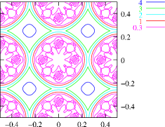
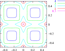
(a)                                     (b)

Figure 15: Contour plot of the two-spinon dispersion $E_{2s}(\boldsymbol{k})$ as a function of $(k_{x}/2\pi,k_{y}/2\pi)$ for the $U(1)$ spin liquid states. (a) is for the $U(1)$-gapless state U1B$0001$ in Eq. (V.4) and (b) is for the $U(1)$-linear state U1B$0011$ in Eq. (V.4).

Due to its long length, we would like to first outline the structure of the paper so readers can choose to read the parts of interests. The section X summarize the main results of the paper, which also serves as a guide of the whole paper. The concept of quantum order is introduced in section I.1. A concrete mathematical description of quantum order is described in section IV.1 and section IV.2. Readers who are interested in the background and motivation of quantum orders may choose to read section I.1. Readers who are familiar with the slave-boson approach and just want a quick introduction to quantum orders may choose to read sections IV.1 and IV.2. Readers who are not familiar with the slave-boson approach may find the review sections II and III useful. Readers who do not care about the slave-boson approach but are interested in application to high $T_{c}$ superconductors and experimental measurements of quantum orders may choose to read sections I.1, I.2, VII and Fig. 1 - Fig. 15, to gain some intuitive picture of spinon dispersion and neutron scattering behavior of various spin liquids.

I.1 Topological orders and quantum orders

Matter can have many different states, such as gas, liquid, and solid. Understanding states of matter is the first step in understanding matter. Physicists find matter can have much more different states than just gas, liquid, and solid. Even solids and liquids can appear in many different forms and states. With so many different states of matter, a general theory is needed to gain a deeper understanding of states of matter.

All the states of matter are distinguished by their internal structures or orders. The key step in developing the general theory for states of matter is the realization that all the orders are associated with symmetries (or rather, the breaking of symmetries). Based on the relation between orders and symmetries, Landau developed a general theory of orders and the transitions between different orders.LL58 ; GL5064 Landau’s theory is so successful and one starts to have a feeling that we understand, at in principle, all kinds of orders that matter can have.

However, nature never stops to surprise us. In 1982, Tsui, Stormer, and GossardTSG8259 discovered a new kind of state – Fractional Quantum Hall (FQH) liquid.L8395 Quantum Hall liquids have many amazing properties. A quantum Hall liquid is more “rigid” than a solid (a crystal), in the sense that a quantum Hall liquid cannot be compressed. Thus a quantum Hall liquid has a fixed and well-defined density. When we measure the electron density in terms of filling factor $\nu$, we found that all discovered quantum Hall states have such densities that the filling factors are exactly given by some rational numbers, such as $\nu=1,1/3,2/3,2/5,...$. Knowing that FQH liquids exist only at certain magical filling factors, one cannot help to guess that FQH liquids should have some internal orders or “patterns”. Different magical filling factors should be due to those different internal “patterns”. However, the hypothesis of internal “patterns” appears to have one difficulty – FQH states are liquids, and how can liquids have any internal “patterns”?

In 1989, it was realized that the internal orders in FQH liquids (as well as the internal orders in chiral spin liquidsKL8795 ; WWZcsp ) are different from any other known orders and cannot be observed and characterized in any conventional ways.Wtop ; WNtop What is really new (and strange) about the orders in chiral spin liquids and FQH liquids is that they are not associated with any symmetries (or the breaking of symmetries), and cannot be described by Landau’s theory using physical order parameters.Wrig This kind of order is called topological order. Topological order is a new concept and a whole new theory was developed to describe it.Wrig ; Wtoprev

Knowing FQH liquids contain a new kind of order – topological order, we would like to ask why FQH liquids are so special. What is missed in Landau’s theory for states of matter so that the theory fails to capture the topological order in FQH liquids?

When we talk about orders in FQH liquids, we are really talking about the internal structure of FQH liquids at zero temperature. In other words, we are talking about the internal structure of the quantum ground state of FQH systems. So the topological order is a property of ground state wave-function. The Landau’s theory is developed for system at finite temperatures where quantum effects can be ignored. Thus one should not be surprised that the Landau’s theory does not apply to states at zero temperature where quantum effects are important. The very existence of topological orders suggests that finite-temperature orders and zero-temperature orders are different, and zero-temperature orders contain richer structures. We see that what is missed by Landau’s theory is simply the quantum effect. Thus FQH liquids are not that special. The Landau’s theory and symmetry characterization can fail for any quantum states at zero temperature. As a consequence, new kind of orders with no broken symmetries and local order parameters (such as topological orders) can exist for any quantum states at zero temperature. Because the orders in quantum states at zero temperature and the orders in classical states at finite temperatures are very different, here we would like to introduce two concepts to stress their differences:Wqos
(A) Quantum orders: which describe the universality classes of quantum ground states (ie the universality classes of complex ground state wave-functions with infinity variables);
(B)Classical orders: which describe the universality classes of classical statistical states (ie the universality classes of positive probability distribution functions with infinity variables).
From the above definition, it is clear that the quantum orders associated with complex functions are richer than the classical orders associated with positive functions. The Landau’s theory is a theory for classical orders, which suggests that classical orders may be characterized by broken symmetries and local order parameters. The existence of topological order indicates that quantum orders cannot be completely characterized by broken symmetries and order parameters. Thus we need to develop a new theory to describe quantum orders.

In a sense, the classical world described by positive probabilities is a world with only “black and white”. The Landau’s theory and the symmetry principle for classical orders are color blind which can only describe different “shades of grey” in the classical world. The quantum world described by complex wave functions is a “colorful” world. We need to use new theories, such as the theory of topological order and the theory developed in this paper, to describe the rich “color” of quantum world.

The quantum orders in FQH liquids have a special property that all excitations above ground state have finite energy gaps. This kind of quantum orders are called topological orders. In general, a topological order is defined as a quantum order where all the excitations above ground state have finite energy gapes.

Topological orders and quantum orders are general properties of any states at zero temperature. Non trivial topological orders not only appear in FQH liquids, they also appear in spin liquids at zero temperature. In fact, the concept of topological order was first introduced in a study of spin liquids.Wrig FQH liquid is not even the first experimentally observed state with non trivial topological orders. That honor goes to superconducting state discovered in 1911.O1122 In contrast to a common point of view, a superconducting state cannot be characterized by broken symmetries. It contains non trivial topological orders,Wtopcs and is fundamentally different from a superfluid state.

After a long introduction, now we can state the main subject of this paper. In this paper, we will study a new class of quantum orders where the excitations above the ground state are gapless. We believe that the gapless quantum orders are important in understanding high $T_{c}$ superconductors. To connect to high $T_{c}$ superconductors, we will study quantum orders in quantum spin liquids on a 2D square lattice. We will concentrate on how to characterize and classify quantum spin liquids with different quantum orders. We introduce projective symmetry groups to help us to achieve this goal. The projective symmetry group can be viewed as a generalization of symmetry group that characterize different classical orders.

I.2 Spin-liquid approach to high $T_{c}$ superconductors

There are many different approaches to the high $T_{c}$ superconductors. Different people have different points of view on what are the key experimental facts for the high $T_{c}$ superconductors. The different choice of the key experimental facts lead to many different approaches and theories. The spin liquid approach is based on a point of view that the high $T_{c}$ superconductors are doped Mott insulators.A8796 ; BZA8773 ; BA8880 (Here by Mott insulator we mean a insulator with an odd number of electron per unit cell.) We believe that the most important properties of the high $T_{c}$ superconductors is that the materials are insulators when the conduction band is half filled. The charge gap obtained by the optical conductance experiments is about $2eV$, which is much larger than the anti-ferromagnetic (AF) transition temperature $T_{\rm AF}\sim 250$K, the superconducting transition temperature $T_{c}\sim 100$K, and the spin pseudo-gap scale $\Delta\sim 40$meV.MDL9641 ; DCN9651 ; MIM9541 The insulating property is completely due to the strong correlations present in the high $T_{c}$ materials. Thus the strong correlations are expect to play very important role in understanding high $T_{c}$ superconductors. Many important properties of high $T_{c}$ superconductors can be directly linked to the Mott insulator at half filling, such as (a) the low charge densityOWT8707 and superfluid density,HBM9399 (b) $T_{c}$ being proportional to doping $T_{c}\propto x$,ULS8917 ; ULL9165 ; KE9534 (c) the positive charge carried by the charge carrier,OWT8707 etc .

In the spin liquid approach, the strategy is to try to understand the properties of the high $T_{c}$ superconductors from the low doping limit. We first study the spin liquid state at half filling and try to understand the parent Mott insulator. (In this paper, by spin liquid, we mean a spin state with translation and spin rotation symmetry.) At half filling, the charge excitations can be ignored due to the huge charge gap. Thus we can use a pure spin model to describe the half filled system. After understand the spin liquid, we try to understand the dynamics of a few doped holes in the spin liquid states and to obtain the properties of the high $T_{c}$ superconductors at low doping. One advantage of the spin liquid approach is that experiments (such as angle resolved photo-emission,MDL9641 ; DCN9651 ; Lo9625 ; HSW9665 NMR,TRH9147 , neutron scattering,MFY0048 ; BSF0034 ; DMH0125 etc ) suggest that underdoped cuperates have many striking and qualitatively new properties which are very different from the well known Fermi liquids. It is thus easier to approve or disapprove a new theory in the underdoped regime by studying those qualitatively new properties.

Since the properties of the doped holes (such as their statistics, spin, effective mass, etc ) are completely determined by the spin correlation in the parent spin liquids, thus in the spin liquid approach, each possible spin liquid leads to a possible theory for high $T_{c}$ superconductors. Using the concept of quantum orders, we can say that possible theories for high $T_{c}$ superconductors in the low doping limits are classified by possible quantum orders in spin liquids on 2D square lattice. Thus one way to study high $T_{c}$ superconductors is to construct all the possible spin liquids that have the same symmetries as those observed in high $T_{c}$ superconductors. Then analyze the physical properties of those spin liquids with dopings to see which one actually describes the high $T_{c}$ superconductor. Although we cannot say that we have constructed all the symmetric spin liquids, in this paper we have found a way to construct a large class of symmetric spin liquids. (Here by symmetric spin liquids we mean spin liquids with all the lattice symmetries: translation, rotation, parity, and the time reversal symmetries.) We also find a way to characterize the quantum orders in those spin liquids via projective symmetry groups. This gives us a global picture of possible high $T_{c}$ theories. We would like to mention that a particular spin liquid – the staggered-flux/$d$-wave stateAM8874 ; KL8842 – may be important for high $T_{c}$ superconductors. Such a state can explainWLsu2 ; RWspec the highly unusual pseudo-gap metallic state found in underdoped cuperates,MDL9641 ; DCN9651 ; Lo9625 ; HSW9665 as well as the $d$-wave superconducting stateKL8842 .

The spin liquids constructed in this paper can be divided into four class: (a) Rigid spin liquid – spinons are fully gaped and may have bosonic, fermionic, or fractional statistics, (b) Fermi spin liquid – spinons are gapless and are described by a Fermi liquid theory, (c) Algebraic spin liquid – spinons are gapless, but they are not described by free fermionic/bosonic quasiparticles. (d) Bose spin liquid – low lying gapless excitations are described by a free boson theory. We find some of the constructed spin liquids are stable and represent stable quantum phases, while others are unstable at low energies due to long range interactions caused by gauge fluctuations. The algebraic spin liquids and Fermi spin liquids are interesting since they can be stable despite their gapless excitations. Those gapless excitations are not protected by symmetries. This is particularly striking for algebraic spin liquids since their gapless excitations interact down to zero energy and the states are still stable. We propose that it is the quantum orders that protect the gapless excitations and ensure the stability of the algebraic spin liquids and Fermi spin liquids.

We would like to point out that both stable and unstable spin liquids may be important for understanding high $T_{c}$ superconductors. Although at zero temperature high $T_{c}$ superconductors are always described stable quantum states, some important states of high $T_{c}$ superconductors, such as the pseudo-gap metallic state for underdoped samples, are observed only at finite temperatures. Such finite temperature states may correspond to (doped) unstable spin liquids, such as staggered flux state. Thus even unstable spin liquids can be useful in understanding finite temperature metallic states.

There are many different approach to spin liquids. In addition to the slave-boson approach,BZA8773 ; BA8880 ; AM8874 ; KL8842 ; SHF8868 ; AZH8845 ; DFM8826 ; WWZcsp ; Wsrvb ; LN9221 ; MF9400 ; WLsu2 spin liquids has been studied using slave-fermion/$\sigma$-model approach,AA8816 ; RS8994 ; RS9173 ; S9277 ; WSC9794 ; SP0114 quantum dimer model,KRS8765 ; RK8876 ; IL8941 ; FK9025 ; MS0181 and various numerical methods.CJZ9062 ; MLB9964 ; CBP0104 ; KI0148 In particular, the numerical results and recent experimental resultsCTT0135 strongly support the existence of quantum spin liquids in some frustrated systems. A 3D quantum orbital liquid was also proposed to exist in $L_{a}T_{i}O_{3}$.KM0050

However, I must point out that there is no generally accepted numerical results yet that prove the existence of spin liquids with odd number of electron per unit cell for spin-1/2 systems, despite intensive search in last ten years. But it is my faith that spin liquids (with odd number of electron per unit cell) exist in spin-1/2 systems. For more general systems, spin liquids do exist. Read and SachdevRS9173 found stable spin liquids in a $Sp(N)$ model in large $N$ limit. The spin-1/2 model studied in this paper can be easily generalized to $SU(N)$ model with $N/2$ fermions per site.AM8874 ; Wlight In the large $N$ limit, one can easily construct various Hamiltonians whose ground states realize various $U(1)$ and $Z_{2}$ spin liquids constructed in this paper.Wtoap The quantum orders in those large-$N$ spin liquids can be described by the methods introduced in this paper. Thus, despite the uncertainty about the existence of spin-1/2 spin liquids, the methods and the results presented in this paper are not about (possibly) non-existing “ghost states”. Those methods and results apply, at least, to certain large-$N$ systems. In short, non-trivial quantum orders exist in theory. We just need to find them in nature. (In fact, our vacuum is likely to be a state with a non-trivial quantum order, due to the fact that light exists.Wlight ) Knowing the existence of spin liquids in large-$N$ systems, it is not such a big leap to go one step further to speculate that spin liquids exist for spin-1/2 systems.

I.3 Spin-charge separation in (doped) spin liquids

Spin-charge separation and the associated gauge theory in spin liquids (and in doped spin liquids) are very important concepts in our attempt to understand the properties of high $T_{c}$ superconductors.A8796 ; BZA8773 ; BA8880 ; IL8988 ; LN9221 However, the exact meaning of spin-charge separation is different for different researchers. The term “spin-charge separation” has at lease in two different interpretations. In the first interpretation, the term means that it is better to introduce separate spinons (a neutral spin-1/2 excitation) and holons (a spinless excitation with unit charge) to understand the dynamical properties of high $T_{c}$ superconductors, instead of using the original electrons. However, there may be long range interaction (possibly, even confining interactions at long distance) between the spinons and holons, and the spinons and holons may not be well defined quasiparticles. We will call this interpretation pseudo spin-charge separation. The algebraic spin liquids have the pseudo spin-charge separation. The essence of the pseudo spin-charge separation is not that spin and charge separate. The pseudo spin-charge separation is simply another way to say that the gapless excitations cannot be described by free fermions or bosons. In the second interpretation, the term “spin-charge separation” means that there are only short ranged interactions between the spinons and holons. The spinons and holons are well defined quasiparticles at least in the dilute limit or at low energies. We will call the second interpretation the true spin-charge separation. The rigid spin liquids and the Fermi spin liquids have the true spin-charge separation.

Electron operator is not a good starting point to describe states with pseudo spin-charge separation or true spin-charge separation. To study those states, we usually rewrite the electron operator as a product of several other operators. Those operators are called parton operators. (The spinon operator and the holon operator are examples of parton operators). We then construct mean-field state in the enlarged Hilbert space of partons. The gauge structure can be determined as the most general transformations between the partons that leave the electron operator unchanged.Wpc After identifying the gauge structure, we can project the mean-field state onto the physical (ie the gauge invariant) Hilbert space and obtain a strongly correlated electron state. This procedure in its general form is called projective construction. It is a generalization of the slave-boson approach.BZA8773 ; BA8880 ; AZH8845 ; DFM8826 ; Wsrvb ; MF9400 ; WLsu2 The general projective construction and the related gauge structure has been discussed in detail for quantum Hall states.Wpc Now we see a third (but technical) meaning of spin-charge separation: to construct a strongly correlated electron state, we need to use partons and projective construction. The resulting effective theory naturally contains a gauge structure.

Although, it is not clear which interpretation of spin-charge separation actually applies to high $T_{c}$ superconductors, the possibility of true spin-charge separation in an electron system is very interesting. The first concrete example of true spin-charge separation in 2D is given by the chiral spin liquid state,KL8795 ; WWZcsp where the gauge interaction between the spinons and holons becomes short-ranged due to a Chern-Simons term. The Chern-Simons term breaks time reversal symmetry and gives the spinons and holons a fractional statistics. Later in 1991, it was realized that there is another way to make the gauge interaction short-ranged through the Anderson-Higgs mechanism.RS9173 ; Wsrvb This led to a mean-field theoryWsrvb ; MF9400 of the short-ranged Resonating Valence Bound (RVB) stateKRS8765 ; RK8876 conjectured earlier. We will call such a state $Z_{2}$ spin liquid state, to stress the unconfined $Z_{2}$ gauge field that appears in the low energy effective theory of those spin liquids. (See remarks at the end of this section. We also note that the $Z_{2}$ spin liquids studied in LABEL:RS9173 all break the $90^{\circ}$ rotation symmetry and are different from the short-ranged RVB state studied LABEL:KRS8765,RK8876,Wsrvb,MF9400.) Since the $Z_{2}$ gauge fluctuations are weak and are not confining, the spinons and holons have only short ranged interactions in the $Z_{2}$ spin liquid state. The $Z_{2}$ spin liquid state also contains a $Z_{2}$ vortex-like excitation.RC8933 ; Wsrvb The spinons and holons can be bosons or fermions depending on if they are bound with the $Z_{2}$ vortex.

Recently, the true spin-charge separation, the $Z_{2}$ gauge structure and the $Z_{2}$ vortex excitations were also proposed in a study of quantum disordered superconducting state in a continuum modelBFN9833 and in a $Z_{2}$ slave-boson approachSF0050 . The resulting liquid state (which was named nodal liquid) has all the novel properties of $Z_{2}$ spin liquid state such as the $Z_{2}$ gauge structure and the $Z_{2}$ vortex excitation (which was named vison). From the point of view of universality class, the nodal liquid is one kind of $Z_{2}$ spin liquids. However, the particular $Z_{2}$ spin liquid studied in LABEL:Wsrvb,MF9400 and the nodal liquid are two different $Z_{2}$ spin liquids, despite they have the same symmetry. The spinons in the first $Z_{2}$ spin liquid have a finite energy gap while the spinons in the nodal liquid are gapless and have a Dirac-like dispersion. In this paper, we will use the projective construction to obtain more general spin liquids. We find that one can construct hundreds of different $Z_{2}$ spin liquids. Some $Z_{2}$ spin liquids have finite energy gaps, while others are gapless. Among those gapless $Z_{2}$ spin liquids, some have finite Fermi surfaces while others have only Fermi points. The spinons near the Fermi points can have linear $E(\boldsymbol{k})\propto|\boldsymbol{k}|$ or quadratic $E(\boldsymbol{k})\propto\boldsymbol{k}^{2}$ dispersions. We find there are more than one $Z_{2}$ spin liquids whose spinons have a massless Dirac-like dispersion. Those $Z_{2}$ spin liquids have the same symmetry but different quantum orders. Their ansatz are give by Eq. (III), Eq. (39), Eq. (88), etc .

Both chiral spin liquid and $Z_{2}$ spin liquid states are Mott insulators with one electron per unit cell if not doped. Their internal structures are characterized by a new kind of order – topological order, if they are gapped or if the gapless sector decouples. Topological order is not related to any symmetries and has no (local) order parameters. Thus, the topological order is robust against all perturbations that can break any symmetries (including random perturbations that break translation symmetry).Wrig ; Wtoprev (This point was also emphasized in LABEL:SF0192 recently.) Even though there are no order parameters to characterize them, the topological orders can be characterized by other measurable quantum numbers, such as ground state degeneracy in compact space as proposed in LABEL:Wrig,Wtoprev. Recently, LABEL:SF0192 introduced a very clever experiment to test the ground state degeneracy associated with the non-trivial topological orders. In addition to ground state degeneracy, there are other practical ways to detect topological orders. For example, the excitations on top of a topologically ordered state can be defects of the under lying topological order, which usually leads to unusual statistics for those excitations. Measuring the statistics of those excitations also allow us to measure topological orders.

The concept of topological order and quantum order are very important in understanding quantum spin liquids (or any other strongly correlated quantum liquids). In this paper we are going to construct hundreds of different spin liquids. Those spin liquids all have the same symmetry. To understand those spin liquids, we need to first learn how to characterize those spin liquids. Those states break no symmetries and hence have no order parameters. One would get into a wrong track if trying to find an order parameter to characterize the spin liquids. We need to use a completely new way, such as topological orders and quantum orders, to characterize those states.

In addition to the above $Z_{2}$ spin liquids, in this paper we will also study many other spin liquids with different low energy gauge structures, such as $U(1)$ and $SU(2)$ gauge structures. We will use the terms $Z_{2}$ spin liquids, $U(1)$ spin liquids, and $SU(2)$ spin liquids to describe them. We would like to stress that $Z_{2}$, $U(1)$, and $SU(2)$ here are gauge groups that appear in the low energy effective theories of those spin liquids. They should not be confused with the $Z_{2}$, $U(1)$, and $SU(2)$ gauge group in slave-boson approach or other theories of the projective construction. The latter are high energy gauge groups. The high energy gauge groups have nothing to do with the low energy gauge groups. A high energy $Z_{2}$ gauge theory (or a $Z_{2}$ slave-boson approach) can have a low energy effective theory that contains $SU(2)$, $U(1)$ or $Z_{2}$ gauge fluctuations. Even the $t$-$J$ model, which has no gauge structure at lattice scale, can have a low energy effective theory that contains $SU(2)$, $U(1)$ or $Z_{2}$ gauge fluctuations. The spin liquids studied in this paper all contain some kind of low energy gauge fluctuations. Despite their different low energy gauge groups, all those spin liquids can be constructed from any one of $SU(2)$, $U(1)$, or $Z_{2}$ slave-boson approaches. After all, all those slave-boson approaches describe the same $t$-$J$ model and are equivalent to each other. In short, the high energy gauge group is related to the way in which we write down the Hamiltonian, while the low energy gauge group is a property of ground state. Thus we should not regard $Z_{2}$ spin liquids as the spin liquids constructed using $Z_{2}$ slave-boson approach. A $Z_{2}$ spin liquid can be constructed from the $U(1)$ or $SU(2)$ slave-boson approaches as well. A precise mathematical definition of the low energy gauge group will be given in section IV.1.

I.4 Organization

In this paper we will use the method outlined in LABEL:Wsrvb,MF9400 to study gauge structures in various spin liquid states. In section II we review $SU(2)$ mean-field theory of spin liquids. In section III, we construct simple symmetric spin liquids using translationally invariant ansatz. In section IV, projective symmetry group is introduced to characterize quantum orders in spin liquids. In section V, we study the transition between different symmetric spin liquids, using the results obtained in appendix B, where we find a way to construct all the symmetric spin liquids in the neighborhood of some well known spin liquids. We also study the spinon spectrum to gain some intuitive understanding on the properties of the spin liquids. Using the relation between two-spinon spectrum and quantum order, we propose, in section VII, a practical way to use neutron scattering to measure quantum orders. We study the stability of Fermi spin liquids and algebraic spin liquids in section VIII. We find that both Fermi spin liquids and algebraic spin liquids can exist as zero temperature phases. This is particularly striking for algebraic spin liquids since their gapless excitations interacts even at lowest energies and there are no free fermionic/bosonic quasiparticle excitations at low energies. We show how quantum order can protect gapless excitations. Appendix A contains a more detailed discussion on projective symmetry group, and a classification of $Z_{2}$, $U(1)$ and $SU(2)$ spin liquids using the projective symmetry group. Section X summarizes the main results of the paper.

II Projective construction of 2D spin liquids – a review of SU(2) slave-boson approach

In this section, we are going to use projective construction to construct 2D spin liquids. We are going to review a particular projective construction, namely the $SU(2)$ slave-boson approach.BZA8773 ; BA8880 ; AZH8845 ; DFM8826 ; Wsrvb ; MF9400 ; WLsu2 The gauge structure discovered by Baskaran and AndersonBA8880 in the slave-boson approach plays a crucial role in our understanding of strongly correlated spin liquids.

We will concentrate on the spin liquid states of a pure spin-1/2 model on a 2D square lattice

$$H_{spin}=\sum_{<\boldsymbol{i}\boldsymbol{j}>}J_{\boldsymbol{i}\boldsymbol{j}}\boldsymbol{S}_{\boldsymbol{i}}\cdot\boldsymbol{S}_{\boldsymbol{j}}+...$$ (1)

where the summation is over different links (ie $\langle\boldsymbol{i}\boldsymbol{j}\rangle$ and $\langle\boldsymbol{j}\boldsymbol{i}\rangle$ are regarded as the same) and $...$ represents possible terms which contain three or more spin operators. Those terms are needed in order for many exotic spin liquid states introduced in this paper to become the ground state. To obtain the mean-field ground state of the spin liquids, we introduce fermionic parton operators $f_{\boldsymbol{i}\alpha},\ \alpha=1,2$ which carries spin $1/2$ and no charge. The spin operator $\boldsymbol{S}_{\boldsymbol{i}}$ is represented as

$$\boldsymbol{S}_{\boldsymbol{i}}=\frac{1}{2}f^{\dagger}_{\boldsymbol{i}\alpha}\boldsymbol{\sigma}_{\alpha\beta}f_{\boldsymbol{i}\beta}$$ (2)

In terms of the fermion operators the Hamiltonian Eq. (1) can be rewritten as

$$H=\sum_{\langle\boldsymbol{i}\boldsymbol{j}\rangle}-\frac{1}{2}J_{\boldsymbol{i}\boldsymbol{j}}\left(f^{\dagger}_{\boldsymbol{i}\alpha}f_{\boldsymbol{j}\alpha}f^{\dagger}_{\boldsymbol{j}\beta}f_{\boldsymbol{i}\beta}+\frac{1}{2}f^{\dagger}_{\boldsymbol{i}\alpha}f_{\boldsymbol{i}\alpha}f^{\dagger}_{\boldsymbol{j}\beta}f_{\boldsymbol{j}\beta}\right)$$ (3)

Here we have used $\boldsymbol{\sigma}_{\alpha\beta}\cdot\boldsymbol{\sigma}_{\alpha^{\prime}\beta^{\prime}}=2\delta_{\alpha\beta^{\prime}}\delta_{\alpha^{\prime}\beta}-\delta_{\alpha\beta}\delta_{\alpha^{\prime}\beta^{\prime}}$. We also added proper constant terms $\sum_{\boldsymbol{i}}f^{\dagger}_{\boldsymbol{i}\alpha}f_{\boldsymbol{i}\alpha}$ and $\sum_{\langle\boldsymbol{i}\boldsymbol{j}\rangle}f^{\dagger}_{\boldsymbol{i}\alpha}f_{\boldsymbol{i}\alpha}f^{\dagger}_{\boldsymbol{j}\beta}f_{\boldsymbol{j}\beta}$ to get the above form. Notice that the Hilbert space of Eq. (3) is generated by the parton operators $f_{\alpha}$ and is larger than that of Eq. (1). The equivalence between Eq. (1) and Eq. (3) is valid only in the subspace where there is exactly one fermion per site. Therefore to use Eq. (3) to describe the spin state we need to impose the constraintBZA8773 ; BA8880

$$f^{\dagger}_{\boldsymbol{i}\alpha}f_{\boldsymbol{i}\alpha}=1,\ \ \ f_{\boldsymbol{i}\alpha}f_{\boldsymbol{i}\beta}\epsilon_{\alpha\beta}=0$$ (4)

The second constraint is actually a consequence of the first one.

A mean-field ground state at “zeroth” order is obtained by making the following approximations. First we replace constraint Eq. (4) by its ground-state average

$$\langle f^{\dagger}_{\boldsymbol{i}\alpha}f_{\boldsymbol{i}\alpha}\rangle=1,\ \ \ \langle f_{\boldsymbol{i}\alpha}f_{\boldsymbol{i}\beta}\epsilon_{\alpha\beta}\rangle=0$$ (5)

Such a constraint can be enforced by including a site dependent and time independent Lagrangian multiplier: $a_{0}^{l}(i)(f^{\dagger}_{\boldsymbol{i}\alpha}f_{\boldsymbol{i}\alpha}-1)$, $l=1,2,3$, in the Hamiltonian. At the zeroth order we ignore the fluctuations (ie the time dependence) of $a_{0}^{l}$. If we included the fluctuations of $a_{0}^{l}$, the constraint Eq. (5) would become the original constraint Eq. (4).BZA8773 ; BA8880 ; AZH8845 ; DFM8826 Second we replace the operators $f^{\dagger}_{\boldsymbol{i}\alpha}f_{\boldsymbol{j}\beta}$ and $f_{\boldsymbol{i}\alpha}f_{\boldsymbol{i}\beta}$ by their ground-state expectations value

$$\eta_{\boldsymbol{i}\boldsymbol{j}}\epsilon_{\alpha\beta}= -2\langle f_{\boldsymbol{i}\alpha}~{}f_{\boldsymbol{j}\beta}\rangle, \eta_{\boldsymbol{i}\boldsymbol{j}}= \eta_{\boldsymbol{j}\boldsymbol{i}}$$

$$\chi_{\boldsymbol{i}\boldsymbol{j}}\delta_{\alpha\beta}= 2\langle f_{\boldsymbol{i}\alpha}^{{\dagger}}f_{\boldsymbol{j}\beta}\rangle, \chi_{\boldsymbol{i}\boldsymbol{j}}= \chi_{\boldsymbol{j}\boldsymbol{i}}^{\dagger}$$ (6)

again ignoring their fluctuations. In this way we obtain the zeroth order mean-field Hamiltonian:

$$H_{mean}$$

$$= \sum_{\langle\boldsymbol{i}\boldsymbol{j}\rangle}-\frac{3}{8}J_{\boldsymbol{i}\boldsymbol{j}}\left[(\chi_{\boldsymbol{j}\boldsymbol{i}}f^{\dagger}_{\boldsymbol{i}\alpha}f_{\boldsymbol{j}\alpha}+\eta_{\boldsymbol{i}\boldsymbol{j}}f^{\dagger}_{i\alpha}f^{\dagger}_{j\beta}~{}\epsilon_{\alpha\beta}+h.c)\right.$$

$$\ \ \ \ \ \ \ \left.-|\chi_{\boldsymbol{i}\boldsymbol{j}}|^{2}-|\eta_{\boldsymbol{i}\boldsymbol{j}}|^{2}\right]$$ (7)

$$+\sum_{\boldsymbol{i}}\left[a_{0}^{3}(f_{\boldsymbol{i}\alpha}^{\dagger}f_{\boldsymbol{i}\alpha}-1)+[(a_{0}^{1}+ia_{0}^{2})f_{\boldsymbol{i}\alpha}f_{\boldsymbol{i}\beta}\epsilon_{\alpha\beta}+h.c.]\right]$$

$\chi_{\boldsymbol{i}\boldsymbol{j}}$ and $\eta_{\boldsymbol{i}\boldsymbol{j}}$ in Eq. (II) must satisfy the self consistency condition Eq. (6) and the site dependent fields $a_{0}^{l}(i)$ are chosen such that Eq. (5) is satisfied by the mean-field ground state. Such $\chi_{\boldsymbol{i}\boldsymbol{j}}$, $\eta_{\boldsymbol{i}\boldsymbol{j}}$ and $a_{0}^{l}$ give us a mean-field solution. The fluctuations in $\chi_{\boldsymbol{i}\boldsymbol{j}}$, $\eta_{\boldsymbol{i}\boldsymbol{j}}$ and $a_{0}^{l}(i)$ describe the collective excitations above the mean-field ground state.

The Hamiltonian Eq. (II) and the constraints Eq. (4) have a local $SU(2)$ symmetry.AZH8845 ; DFM8826 The local $SU(2)$ symmetry becomes explicit if we introduce doublet

$$\psi=\begin{pmatrix}\psi_{1}\\ \psi_{2}\end{pmatrix}=\begin{pmatrix}f_{\uparrow}\\ f_{\downarrow}^{\dagger}\end{pmatrix}$$ (8)

and matrix

$$U_{\boldsymbol{i}\boldsymbol{j}}=\begin{pmatrix}\chi_{\boldsymbol{i}\boldsymbol{j}}^{\dagger}&\eta_{\boldsymbol{i}\boldsymbol{j}}\\ \eta_{\boldsymbol{i}\boldsymbol{j}}^{\dagger}&-\chi_{\boldsymbol{i}\boldsymbol{j}}\end{pmatrix}=U_{\boldsymbol{j}\boldsymbol{i}}^{\dagger}$$ (9)

Using Eq. (8) and Eq. (9) we can rewrite Eq. (5) and Eq. (II) as:

$$\left\langle\psi_{\boldsymbol{i}}^{\dagger}\tau^{l}\psi_{\boldsymbol{i}}\right\rangle=0$$ (10)

$$H_{mean}= \sum_{\langle\boldsymbol{i}\boldsymbol{j}\rangle}\frac{3}{8}J_{\boldsymbol{i}\boldsymbol{j}}\left[\frac{1}{2}{\rm Tr}(U_{\boldsymbol{i}\boldsymbol{j}}^{\dagger}~{}U_{\boldsymbol{i}\boldsymbol{j}})-(\psi^{\dagger}_{i}U_{\boldsymbol{i}\boldsymbol{j}}\psi_{j}+~{}h.c.)\right]$$

$$+\sum_{\boldsymbol{i}}a_{0}^{l}\psi_{\boldsymbol{i}}^{\dagger}\tau^{l}\psi_{\boldsymbol{i}}$$ (11)

where $\tau^{l},\ l=1,2,3$ are the Pauli matrices. From Eq. (11) we can see clearly that the Hamiltonian is invariant under a local $SU(2)$ transformation $W(\boldsymbol{i})$:

$$\psi_{\boldsymbol{i}} \to W(\boldsymbol{i})~{}\psi_{\boldsymbol{i}}$$

$$U_{\boldsymbol{i}\boldsymbol{j}} \to W(\boldsymbol{i})~{}U_{\boldsymbol{i}\boldsymbol{j}}~{}W^{\dagger}(\boldsymbol{j})$$ (12)

The $SU(2)$ gauge structure is originated from Eq. (2). The $SU(2)$ is the most general transformation between the partons that leave the physical spin operator unchanged. Thus once we write down the parton expression of the spin operator Eq. (2), the gauge structure of the theory is determined.Wpc (The $SU(2)$ gauge structure discussed here is a high energy gauge structure.)

We note that both components of $\psi$ carry spin-up. Thus the spin-rotation symmetry is not explicit in our formalism and it is hard to tell if Eq. (11) describes a spin-rotation invariant state or not. In fact, for a general $U_{\boldsymbol{i}\boldsymbol{j}}$ satisfying $U_{\boldsymbol{i}\boldsymbol{j}}=U_{\boldsymbol{j}\boldsymbol{i}}^{\dagger}$, Eq. (11) may not describe a spin-rotation invariant state. However, if $U_{\boldsymbol{i}\boldsymbol{j}}$ has a form

$$U_{\boldsymbol{i}\boldsymbol{j}} = i\rho_{\boldsymbol{i}\boldsymbol{j}}W_{\boldsymbol{i}\boldsymbol{j}},$$

$$\rho_{\boldsymbol{i}\boldsymbol{j}} = \hbox{real number},$$

$$W_{\boldsymbol{i}\boldsymbol{j}} \in SU(2),$$ (13)

then Eq. (11) will describe a spin-rotation invariant state. This is because the above $U_{\boldsymbol{i}\boldsymbol{j}}$ can be rewritten in a form Eq. (9). In this case Eq. (11) can be rewritten as Eq. (II) where the spin-rotation invariance is explicit.

To obtain the mean-field theory, we have enlarged the Hilbert space. Because of this, the mean-field theory is not even qualitatively correct. Let $|\Psi_{mean}^{(U_{\boldsymbol{i}\boldsymbol{j}})}\rangle$ be the ground state of the Hamiltonian Eq. (11) with energy $E(U_{\boldsymbol{i}\boldsymbol{j}},a^{l}_{\boldsymbol{i}}\tau^{l})$. It is clear that the mean-field ground state is not even a valid wave-function for the spin system since it may not have one fermion per site. Thus it is very important to include fluctuations of $a_{0}^{l}$ to enforce one-fermion-per-site constraint. With this understanding, we may obtain a valid wave-function of the spin system $\Psi_{spin}(\{\alpha_{\boldsymbol{i}}\})$ by projecting the mean-field state to the subspace of one-fermion-per-site:

$$\Psi_{spin}(\{\alpha_{\boldsymbol{i}}\})=\langle 0|\prod_{\boldsymbol{i}}f_{\boldsymbol{i}\alpha_{\boldsymbol{i}}}|\Psi_{mean}^{(U_{\boldsymbol{i}\boldsymbol{j}})}\rangle.$$ (14)

Now the local $SU(2)$ transformation Eq. (12) can have a very physical meaning: $|\Psi_{mean}^{(U_{\boldsymbol{i}\boldsymbol{j}})}\rangle$ and $|\Psi_{mean}^{(W(\boldsymbol{i})U_{\boldsymbol{i}\boldsymbol{j}}W^{\dagger}(\boldsymbol{j}))}\rangle$ give rise to the same spin wave-function after projection:

$$\langle 0|\prod_{\boldsymbol{i}}f_{\boldsymbol{i}\alpha_{\boldsymbol{i}}}|\Psi_{mean}^{(U_{\boldsymbol{i}\boldsymbol{j}})}\rangle=\langle 0|\prod_{\boldsymbol{i}}f_{\boldsymbol{i}\alpha_{\boldsymbol{i}}}|\Psi_{mean}^{(W(\boldsymbol{i})U_{\boldsymbol{i}\boldsymbol{j}}W^{\dagger}(\boldsymbol{j}))}\rangle$$ (15)

Thus $U_{\boldsymbol{i}\boldsymbol{j}}$ and $U^{\prime}_{\boldsymbol{i}\boldsymbol{j}}=W(\boldsymbol{i})U_{\boldsymbol{i}\boldsymbol{j}}W^{\dagger}(\boldsymbol{j})$ are just two different labels which label the same physical state. Within the mean-field theory, a local $SU(2)$ transformation changes a mean-field state $|\Psi_{mean}^{(U_{\boldsymbol{i}\boldsymbol{j}})}\rangle$ to a different mean-field state $|\Psi_{mean}^{(U^{\prime}_{\boldsymbol{i}\boldsymbol{j}})}\rangle$. If the two mean-field states always have the same physical properties, the system has a local $SU(2)$ symmetry. However, after projection, the physical spin quantum state described by wave-function $\Psi_{spin}(\{\alpha_{\boldsymbol{i}}\})$ is invariant under the local $SU(2)$ transformation. A local $SU(2)$ transformation just transforms one label, $U_{\boldsymbol{i}\boldsymbol{j}}$, of a physical spin state to another label, $U^{\prime}_{\boldsymbol{i}\boldsymbol{j}}$, which labels the exactly the same physical state. Thus after projection, local $SU(2)$ transformations become gauge transformations. The fact that $U_{\boldsymbol{i}\boldsymbol{j}}$ and $U^{\prime}_{\boldsymbol{i}\boldsymbol{j}}$ label the same physical spin state creates a interesting situation when we consider the fluctuations of $U_{\boldsymbol{i}\boldsymbol{j}}$ around a mean-field solution – some fluctuations of $U_{\boldsymbol{i}\boldsymbol{j}}$ do not change the physical state and are unphysical. Those fluctuations are called the pure gauge fluctuations.

The above discussion also indicates that in order for the mean-field theory to make any sense, we must at least include the $SU(2)$ gauge (or other gauge) fluctuations described by $a_{0}^{l}$ and $W_{\boldsymbol{i}\boldsymbol{j}}$ in Eq. (II), so that the $SU(2)$ gauge structure of the mean-field theory is revealed and the physical spin state is obtained. We will include the gauge fluctuations to the zeroth-order mean-field theory. The new theory will be called the first order mean-field theory. It is this first order mean-field theory that represents a proper low energy effective theory of the spin liquid.

Here, we would like make a remark about “gauge symmetry” and “gauge symmetry breaking”. We see that two ansatz $U_{\boldsymbol{i}\boldsymbol{j}}$ and $U^{\prime}_{\boldsymbol{i}\boldsymbol{j}}=W(\boldsymbol{i})U_{\boldsymbol{i}\boldsymbol{j}}W^{\dagger}(\boldsymbol{j})$ have the same physical properties. This property is usually called the “gauge symmetry”. However, from the above discussion, we see that the “gauge symmetry” is not a symmetry. A symmetry is about two different states having the same properties. $U_{\boldsymbol{i}\boldsymbol{j}}$ and $U^{\prime}_{\boldsymbol{i}\boldsymbol{j}}$ are just two labels that label the same state, and the same state always have the same properties. We do not usually call the same state having the same properties a symmetry. Because the same state alway have the same properties, the “gauge symmetry” can never be broken. It is very misleading to call the Anderson-Higgs mechanism “gauge symmetry breaking”. With this understanding, we see that a superconductor is fundamentally different from a superfluid. A superfluid is characterized by $U(1)$ symmetry breaking, while a superconductor has no symmetry breaking once we include the dynamical electromagnetic gauge fluctuations. A superconductor is actually the first topologically ordered state observed in experiments,Wtopcs which has no symmetry breaking, no long range order, and no (local) order parameter. However, when the speed of light $c=\infty$, a superconductor becomes similar to a superfluid and is characterized by $U(1)$ symmetry breaking.

The relation between the mean-field state and the physical spin wave function Eq. (14) allows us to construct transformation of the physical spin wave-function from the mean-field ansatz. For example the mean-field state $|\Psi_{mean}^{(U^{\prime}_{\boldsymbol{i}\boldsymbol{j}})}\rangle$ with $U^{\prime}_{\boldsymbol{i}\boldsymbol{j}}=U_{\boldsymbol{i}-\boldsymbol{l},\boldsymbol{j}-\boldsymbol{l}}$ produces a physical spin wave-function which is translated by a distance $\boldsymbol{l}$ from the physical spin wave-function produced by $|\Psi_{mean}^{(U_{\boldsymbol{i}\boldsymbol{j}})}\rangle$. The physical state is translationally symmetric if and only if the translated ansatz $U^{\prime}_{\boldsymbol{i}\boldsymbol{j}}$ and the original ansatz $U_{\boldsymbol{i}\boldsymbol{j}}$ are gauge equivalent (it does not require $U^{\prime}_{\boldsymbol{i}\boldsymbol{j}}=U_{\boldsymbol{i}\boldsymbol{j}}$). We see that the gauge structure can complicates our analysis of symmetries, since the physical spin wave-function $\Psi_{spin}(\{\alpha_{\boldsymbol{i}}\})$ may has more symmetries than the mean-field state $|\Psi_{mean}^{(U_{\boldsymbol{i}\boldsymbol{j}})}\rangle$ before projection.

Let us discuss time reversal symmetry in more detail. A quantum system described by

$$i\hbar\partial_{t}\Psi(t)=H\Psi(t)$$ (16)

has a time reversal symmetry if $\Psi(t)$ satisfying the equation of motion implies that $\Psi^{*}(-t)$ also satisfying the equation of motion. This requires that $H=H^{*}$. We see that, for time reversal symmetric system, if $\Psi$ is an eigenstate, then $\Psi^{*}$ will be an eigenstate with the same energy.

For our system, the time reversal symmetry means that if the mean-field wave function $\Psi_{mean}^{(U_{\boldsymbol{i}\boldsymbol{j}},a^{l}_{\boldsymbol{i}}\tau^{l})}$ is a mean-field ground state wave function for ansatz $(U_{\boldsymbol{i}\boldsymbol{j}},a^{l}_{\boldsymbol{i}}\tau^{l})$, then $\left(\Psi_{mean}^{(U_{\boldsymbol{i}\boldsymbol{j}},a^{l}_{\boldsymbol{i}}\tau^{l})}\right)^{*}$ will be the mean-field ground state wave function for ansatz $(U^{*}_{\boldsymbol{i}\boldsymbol{j}},a^{l}_{\boldsymbol{i}}(\tau^{l})^{*})$. That is

$$\left(\Psi_{mean}^{(U_{\boldsymbol{i}\boldsymbol{j}},a^{l}_{\boldsymbol{i}}\tau^{l})}\right)^{*}=\Psi_{mean}^{(U^{*}_{\boldsymbol{i}\boldsymbol{j}},a^{l}_{\boldsymbol{i}}(\tau^{l})^{*})}$$ (17)

For a system with time reversal symmetry, the mean-field energy $E(U_{\boldsymbol{i}\boldsymbol{j}},a^{l}_{\boldsymbol{i}}\tau^{l})$ satisfies

$$E(U_{\boldsymbol{i}\boldsymbol{j}},a^{l}_{\boldsymbol{i}}\tau^{l})=E(U^{*}_{\boldsymbol{i}\boldsymbol{j}},a^{l}_{\boldsymbol{i}}(\tau^{l})^{*})$$ (18)

Thus if an ansatz $(U_{\boldsymbol{i}\boldsymbol{j}},a_{\boldsymbol{i}}^{l}\tau^{l})$ is a mean-field solution, then $(U^{*}_{\boldsymbol{i}\boldsymbol{j}},a_{\boldsymbol{i}}^{l}(\tau^{l})^{*})$ is also a mean-field solution with the same mean-field energy.

From the above discussion, we see that under the time reversal transformation, the ansatz transforms as

$$U_{\boldsymbol{i}\boldsymbol{j}} \to U_{\boldsymbol{i}\boldsymbol{j}}^{\prime}=(-i\tau^{2})U_{\boldsymbol{i}\boldsymbol{j}}^{*}(i\tau^{2})=-U_{\boldsymbol{i}\boldsymbol{j}},$$

$$a_{\boldsymbol{i}}^{l}\tau^{l} \to a_{\boldsymbol{i}}^{\prime l}\tau^{l}=(-i\tau^{2})(a_{\boldsymbol{i}}^{l}\tau^{l})^{*}(i\tau^{2})=-a_{\boldsymbol{i}}^{l}\tau^{l}.$$ (19)

Note here we have included an additional $SU(2)$ gauge transformation $W_{\boldsymbol{i}}=-i\tau^{2}$. We also note that under the time reversal transformation, the loop operator transforms as $P_{C}=e^{i\theta+i\theta^{l}\tau^{l}}\to(-i\tau^{2})P_{C}^{*}(i\tau^{2})=e^{-i\theta+i\theta^{l}\tau^{l}}$. We see that the $U(1)$ flux changes the sign while the $SU(2)$ flux is not changed.

Before ending this review section, we would like to point out that the mean-field ansatz of the spin liquids $U_{\boldsymbol{i}\boldsymbol{j}}$ can be divided into two classes: unfrustrated ansatz where $U_{\boldsymbol{i}\boldsymbol{j}}$ only link an even lattice site to an odd lattice site and frustrated ansatz where $U_{\boldsymbol{i}\boldsymbol{j}}$ are nonzero between two even sites and/or two odd sites. An unfrustrated ansatz has only pure $SU(2)$ flux through each plaquette, while an frustrated ansatz has $U(1)$ flux of multiple of $\pi/2$ through some plaquettes in addition to the $SU(2)$ flux.

III Spin liquids from translationally invariant ansatz

In this section, we will study many simple examples of spin liquids and their ansatz. Through those simple examples, we gain some understandings on what kind of spin liquids are possible. Those understandings help us to develop the characterization and classification of spin liquids using projective symmetry group.

Using the above $SU(2)$ projective construction, one can construct many spin liquid states. To limit ourselves, we will concentrate on spin liquids with translation and $90^{\circ}$ rotation symmetries. Although a mean-field ansatz with translation and rotation invariance always generate a spin liquid with translation and rotation symmetries, a mean-field ansatz without those invariances can also generate a spin liquid with those symmetries. Because of this, it is quite difficult to construct all the translation and rotation symmetric spin liquids. In this section we will consider a simpler problem. We will limit ourselves to spin liquids generated from translationally invariant ansatz:

$$U_{\boldsymbol{i}+\boldsymbol{l},\boldsymbol{j}+\boldsymbol{l}}=U_{\boldsymbol{i}\boldsymbol{j}},\ \ \ \ a_{0}^{l}(\boldsymbol{i})=a_{0}^{l}$$ (20)

In this case, we only need to find the conditions under which the above ansatz can give rise to a rotationally symmetric spin liquid. First let us introduce $u_{\boldsymbol{i}\boldsymbol{j}}$:

$$\frac{3}{8}J_{\boldsymbol{i}\boldsymbol{j}}U_{\boldsymbol{i}\boldsymbol{j}}=u_{\boldsymbol{i}\boldsymbol{j}}$$ (21)

For translationally invariant ansatz, we can introduce a short-hand notation:

$$u_{\boldsymbol{i}\boldsymbol{j}}=u_{-\boldsymbol{i}+\boldsymbol{j}}^{\mu}\tau^{\mu}\equiv u_{-\boldsymbol{i}+\boldsymbol{j}}$$ (22)

where $u_{\boldsymbol{l}}^{1,2,3}$ are real, $u_{\boldsymbol{l}}^{0}$ is imaginary, $\tau^{0}$ is the identity matrix and $\tau^{1,2,3}$ are the Pauli matrices. The fermion spectrum is determined by Hamiltonian

$$H= -\sum_{\langle\boldsymbol{i}\boldsymbol{j}\rangle}\left(\psi^{\dagger}_{\boldsymbol{i}}u_{\boldsymbol{j}-\boldsymbol{i}}\psi_{\boldsymbol{j}}+h.c.\right)+\sum_{\boldsymbol{i}}\psi^{\dagger}_{\boldsymbol{i}}a_{0}^{l}\tau^{l}\psi_{\boldsymbol{i}}$$ (23)

In $\boldsymbol{k}$-space we have

$$H=-\sum_{\boldsymbol{k}}\psi^{\dagger}_{\boldsymbol{k}}(u^{\mu}(\boldsymbol{k})-a_{0}^{\mu})\tau^{\mu}\psi_{\boldsymbol{k}}$$ (24)

where $\mu=0,1,2,3$,

$$u^{\mu}(\boldsymbol{k})=\sum_{\boldsymbol{l}}u^{\mu}_{\boldsymbol{l}}e^{i\boldsymbol{l}\cdot\boldsymbol{k}},$$ (25)

$a_{0}^{0}=0$, and $N$ is the total number of site. The fermion spectrum has two branches and is given by

$$E_{\pm}(\boldsymbol{k})= u^{0}(\boldsymbol{k})\pm E_{0}(\boldsymbol{k})$$

$$E_{0}(\boldsymbol{k})= \sqrt{\sum_{l}(u^{l}(\boldsymbol{k})-a_{0}^{l})^{2}}$$ (26)

The constraints can be obtained from $\frac{\partial E_{ground}}{\partial a_{0}^{l}}=0$ and have a form

$$N\langle\psi_{\boldsymbol{i}}^{\dagger}\tau^{l}\psi_{\boldsymbol{i}}\rangle$$

$$= \sum_{\boldsymbol{k},E_{-}(\boldsymbol{k})<0}\frac{u^{l}(\boldsymbol{k})-a_{0}^{l}}{E_{0}(\boldsymbol{k})}-\sum_{\boldsymbol{k},E_{+}(\boldsymbol{k})<0}\frac{u^{l}(\boldsymbol{k})-a_{0}^{l}}{E_{0}(\boldsymbol{k})}=0$$ (27)

which allow us to determine $a_{0}^{l}$, $l=1,2,3$. It is interesting to see that if $u^{0}_{\boldsymbol{i}}=0$ and the ansatz is unfrustrated, then we can simply choose $a_{0}^{l}=0$ to satisfy the mean-field constraints (since $u^{\mu}(\boldsymbol{k})=-u^{\mu}(\boldsymbol{k}+(\pi,\pi))$ for unfrustrated ansatz). Such ansatz always have time reversal symmetry. This is because $U_{\boldsymbol{i}\boldsymbol{j}}$ and $-U_{\boldsymbol{i}\boldsymbol{j}}$ are gauge equivalent for unfrustrated ansatz.

Now let us study some simple examples. First let us assume that only the nearest neighbor coupling $u_{\hat{\boldsymbol{x}}}$ and $u_{\hat{\boldsymbol{y}}}$ are non-zero. In order for the ansatz to describe a rotationally symmetric state, the rotated ansatz must be gauge equivalent to the original ansatz. One can easily check that the following ansatz has the rotation symmetry

$$a_{0}^{l} = 0$$

$$u_{\hat{\boldsymbol{x}}} = \chi\tau^{3}+\eta\tau^{1}$$

$$u_{\hat{\boldsymbol{y}}} = \chi\tau^{3}-\eta\tau^{1}$$ (28)

since the $90^{\circ}$ rotation followed by a gauge transformation $W_{\boldsymbol{i}}=i\tau^{3}$ leave the ansatz unchanged. The above ansatz also has the time reversal symmetry, since time reversal transformation $u_{\boldsymbol{i}\boldsymbol{j}}\to-u_{\boldsymbol{i}\boldsymbol{j}}$ followed by a gauge transformation $W_{\boldsymbol{i}}=i\tau^{2}$ leave the ansatz unchanged.

To understand the gauge fluctuations around the above mean-field state, we note that the mean-field ansatz may generate non-trivial $SU(2)$ flux through plaquettes. Those flux may break $SU(2)$ gauge structure down to $U(1)$ or $Z_{2}$ gauge structures as discussed in LABEL:Wsrvb,MF9400. In particular, the dynamics of the gauge fluctuations in the break down from $SU(2)$ to $Z_{2}$ has been discussed in detail in LABEL:MF9400. According to LABEL:Wsrvb,MF9400, the $SU(2)$ flux plays a role of Higgs fields. A non-trivial $SU(2)$ flux correspond to a condensation of Higgs fields which can break the gauge structure and give $SU(2)$ and/or $U(1)$ gauge boson a mass. Thus to understand the dynamics of the gauge fluctuations, we need to find the $SU(2)$ flux.

The $SU(2)$ flux is defined for loops with a base point. The loop starts and ends at the base point. For example, we can consider the following two loops $C_{1,2}$ with the same base point $\boldsymbol{i}$: $C_{1}=\boldsymbol{i}\to\boldsymbol{i}+\hat{\boldsymbol{x}}\to\boldsymbol{i}+\hat{\boldsymbol{x}}+\hat{\boldsymbol{y}}\to\boldsymbol{i}+\hat{\boldsymbol{y}}\to\boldsymbol{i}$ and $C_{2}$ is the 90^∘ rotation of $C_{1}$: $C_{2}=\boldsymbol{i}\to\boldsymbol{i}+\hat{\boldsymbol{y}}\to\boldsymbol{i}-\hat{\boldsymbol{x}}+\hat{\boldsymbol{y}}\to\boldsymbol{i}-\hat{\boldsymbol{x}}\to\boldsymbol{i}$. The $SU(2)$ flux for the two loops is defined as

$$P_{C_{1}}\equiv u_{\boldsymbol{i},\boldsymbol{i}+\hat{\boldsymbol{y}}}u_{\boldsymbol{i}+\hat{\boldsymbol{y}},\boldsymbol{i}+\hat{\boldsymbol{x}}+\hat{\boldsymbol{y}}}u_{\boldsymbol{i}+\hat{\boldsymbol{x}}+\hat{\boldsymbol{y}},\boldsymbol{i}+\hat{\boldsymbol{x}}}u_{\boldsymbol{i}+\hat{\boldsymbol{x}},\boldsymbol{i}}=u_{\hat{\boldsymbol{y}}}^{\dagger}u_{\hat{\boldsymbol{x}}}^{\dagger}u_{\hat{\boldsymbol{y}}}u_{\hat{\boldsymbol{x}}}$$

$$P_{C_{2}}\equiv u_{\boldsymbol{i},\boldsymbol{i}-\hat{\boldsymbol{x}}}u_{\boldsymbol{i}-\hat{\boldsymbol{x}},\boldsymbol{i}-\hat{\boldsymbol{x}}+\hat{\boldsymbol{y}}}u_{\boldsymbol{i}-\hat{\boldsymbol{x}}+\hat{\boldsymbol{y}},\boldsymbol{i}+\hat{\boldsymbol{y}}}u_{\boldsymbol{i}+\hat{\boldsymbol{y}},\boldsymbol{i}}=u_{\hat{\boldsymbol{x}}}u_{\hat{\boldsymbol{y}}}^{\dagger}u_{\hat{\boldsymbol{x}}}^{\dagger}u_{\hat{\boldsymbol{y}}}$$ (29)

As discussed in LABEL:Wsrvb,MF9400, if the $SU(2)$ flux $P_{C}$ for all loops are trivial: $P_{C}\propto\tau^{0}$, then the $SU(2)$ gauge structure is unbroken. This is the case when $\chi=\eta$ or when $\eta=0$ in the above ansatz Eq. (28). The spinon in the spin liquid described by $\eta=0$ has a large Fermi surface. We will call this state $SU(2)$-gapless state (This state was called uniform RVB state in literature). The state with $\chi=\eta$ has gapless spinons only at isolated $\boldsymbol{k}$ points. We will call such a state $SU(2)$-linear state to stress the linear dispersion $E\propto|\boldsymbol{k}|$ near the Fermi points. (Such a state was called the $\pi$-flux state in literature). The low energy effective theory for the $SU(2)$-linear state is described by massless Dirac fermions (the spinons) coupled to a $SU(2)$ gauge field.

After proper gauge transformations, the $SU(2)$-gapless ansatz can be rewritten as

$$u_{\hat{\boldsymbol{x}}} = i\chi$$

$$u_{\hat{\boldsymbol{y}}} = i\chi$$ (30)

and the $SU(2)$-linear ansatz as

$$u_{\boldsymbol{i},\boldsymbol{i}+\hat{\boldsymbol{x}}} = i\chi$$

$$u_{\boldsymbol{i},\boldsymbol{i}+\hat{\boldsymbol{y}}} = i(-)^{i_{x}}\chi$$ (31)

In these form, the $SU(2)$ gauge structure is explicit since $u_{\boldsymbol{i}\boldsymbol{j}}\propto i\tau^{0}$. Here we would also like to mention that under the projective-symmetry-group classification, the $SU(2)$-gapless ansatz Eq. (III) is labeled by SU2A$n0$ and the $SU(2)$-linear ansatz Eq. (III) by SU2B$n0$ (see Eq. (IV.3)).

When $\chi\neq\eta\neq 0$, The flux $P_{C}$ is non trivial. However, $P_{C}$ commute with $P_{C^{\prime}}$ as long as the two loops $C$ and $C^{\prime}$ have the same base point. In this case the $SU(2)$ gauge structure is broken down to a $U(1)$ gauge structure.Wsrvb ; MF9400 The gapless spinon still only appear at isolated $\boldsymbol{k}$ points. We will call such a state $U(1)$-linear state. (This state was called staggered flux state and/or $d$-wave pairing state in literature.) After a proper gauge transformation, the $U(1)$-linear state can also be described by the ansatz

$$u_{\boldsymbol{i},\boldsymbol{i}+\hat{\boldsymbol{x}}}=i\chi-(-)^{\boldsymbol{i}}\eta\tau^{3}$$

$$u_{\boldsymbol{i},\boldsymbol{i}+\hat{\boldsymbol{y}}}=i\chi+(-)^{\boldsymbol{i}}\eta\tau^{3}$$ (32)

where the $U(1)$ gauge structure is explicit. Under the projective-symmetry-group classification, such a state is labeled by U1C$n01n$ (see Eq. (B.3) and IV.3). The low energy effective theory is described by massless Dirac fermions (the spinons) coupled to a $U(1)$ gauge field.

The above results are all known before. In the following we are going to study a new class of translation and rotation symmetric ansatz, which has a form

$$a_{0}^{l}= 0$$

$$u_{\hat{\boldsymbol{x}}}= i\eta\tau^{0}-\chi(\tau^{3}-\tau^{1})$$

$$u_{\hat{\boldsymbol{y}}}= i\eta\tau^{0}-\chi(\tau^{3}+\tau^{1})$$ (33)

with $\chi$ and $\eta$ non-zero. The above ansatz describes the $SU(2)$-gapless spin liquid if $\chi=0$, and the $SU(2)$-linear spin liquid if $\eta=0$.

After a $90^{\circ}$ rotation $R_{90}$, the above ansatz becomes

$$u_{\hat{\boldsymbol{x}}} = -i\eta\tau^{0}-\chi(\tau^{3}+\tau^{1})$$

$$u_{\hat{\boldsymbol{y}}} = i\eta\tau^{0}-\chi(\tau^{3}-\tau^{1})$$ (34)

The rotated ansatz is gauge equivalent to the original ansatz under the gauge transformation $G_{R_{90}}(\boldsymbol{i})=(-)^{i_{x}}(1-i\tau^{2})/\sqrt{2}$. After a parity $x\to-x$ transformation $P_{x}$, Eq. (III) becomes

$$u_{\hat{\boldsymbol{x}}}=-i\eta\tau^{0}-\chi(\tau^{3}-\tau^{1})$$

$$u_{\hat{\boldsymbol{y}}}=i\eta\tau^{0}-\chi(\tau^{3}+\tau^{1})$$ (35)

which is gauge equivalent to the original ansatz under the gauge transformation $G_{P_{x}}(\boldsymbol{i})=(-)^{i_{x}}i(\tau^{3}+\tau^{1})/\sqrt{2}$. Under time reversal transformation $T$, Eq. (III) is changed to

$$u_{\hat{\boldsymbol{x}}}=-i\eta\tau^{0}+\chi(\tau^{3}-\tau^{1})$$

$$u_{\hat{\boldsymbol{y}}}=-i\eta\tau^{0}+\chi(\tau^{3}+\tau^{1})$$ (36)

which is again gauge equivalent to the original ansatz under the gauge transformation $G_{T}(\boldsymbol{i})=(-)^{\boldsymbol{i}}$. (In fact any ansatz which only has links between two non-overlapping sublattices (ie the unfrustrated ansatz) is time reversal symmetric if $a_{0}^{l}=0$ .) To summarize the ansatz Eq. (III) is invariant under the rotation $R_{90}$, parity $P_{x}$, and time reversal transformation $T$, followed by the following gauge transformations

$$G_{R_{90}}(\boldsymbol{i})= (-)^{i_{x}}(1-i\tau^{2})/\sqrt{2}$$

$$G_{P_{x}}(\boldsymbol{i})= (-)^{i_{x}}i(\tau^{3}+\tau^{1})/\sqrt{2}$$

$$G_{T}(\boldsymbol{i})= (-)^{\boldsymbol{i}}$$ (37)

Thus the ansatz Eq. (III) describes a spin liquid which translation, rotation, parity and time reversal symmetries.

Using the time reversal symmetry we can show that the vanishing $a_{0}^{l}$ in our ansatz Eq. (III) indeed satisfy the constraint Eq. (27). This is because $a_{0}^{l}\to-a_{0}^{l}$ under the time reversal transformation. Thus $\frac{\partial E_{mean}}{\partial a_{0}^{l}}=0$ when $a^{l}_{0}=0$ for any time reversal symmetric ansatz, including the ansatz Eq. (III).

The spinon spectrum is given by (see Fig. 5a)

$$E_{\pm}=2\eta(\sin(k_{x})+\sin(k_{y}))\pm 2|\chi|\sqrt{2\cos^{2}(k_{x})+2\cos^{2}(k_{y})}$$ (38)

The spinons have two Fermi points and two small Fermi pockets (for small $\eta$). The $SU(2)$ flux is non-trivial. Further more $P_{C_{1}}$ and $P_{C_{2}}$ do not commute. Thus the $SU(2)$ gauge structure is broken down to a $Z_{2}$ gauge structure by the $SU(2)$ flux $P_{C_{1}}$ and $P_{C_{2}}$.Wsrvb ; MF9400 We will call the spin liquid described by Eq. (III) $Z2$-gapless spin liquid. The low energy effective theory is described by massless Dirac fermions and fermions with small Fermi surfaces, coupled to a $Z_{2}$ gauge field. Since the $Z_{2}$ gauge interaction is irrelevant at low energies, the spinons are free fermions at low energies and we have a true spin-charge separation in the $Z_{2}$-gapless spin liquid. The $Z_{2}$-gapless spin liquid is one of the $Z_{2}$ spin liquids classified in appendix A. Its projective symmetry group is labeled by Z2A$\tau^{13}_{-}\tau^{1\bar{3}}_{+}\tau^{3}\tau^{0}_{-}$ or equivalently by Z2A$x2(12)n$ (see section IV.2 and Eq. (67)).

Now let us include longer links. First we still limit ourselves to unfrustrated ansatz. An interesting ansatz is given by

$$a_{0}^{l} = 0$$

$$u_{\hat{\boldsymbol{x}}} = \chi\tau^{3}+\eta\tau^{1}$$

$$u_{\hat{\boldsymbol{y}}} = \chi\tau^{3}-\eta\tau^{1}$$

$$u_{2\hat{\boldsymbol{x}}+\hat{\boldsymbol{y}}} = \lambda\tau^{2}$$

$$u_{-\hat{\boldsymbol{x}}+2\hat{\boldsymbol{y}}} = -\lambda\tau^{2}$$

$$u_{2\hat{\boldsymbol{x}}-\hat{\boldsymbol{y}}} = \lambda\tau^{2}$$

$$u_{\hat{\boldsymbol{x}}+2\hat{\boldsymbol{y}}} = -\lambda\tau^{2}$$ (39)

By definition, the ansatz is invariant under translation and parity $x\to-x$. After a $90^{\circ}$ rotation, the ansatz is changed to

$$u_{\hat{\boldsymbol{x}}} = -\chi\tau^{3}-\eta\tau^{1}$$

$$u_{\hat{\boldsymbol{y}}} = -\chi\tau^{3}+\eta\tau^{1}$$

$$u_{2\hat{\boldsymbol{x}}+\hat{\boldsymbol{y}}} = -\lambda\tau^{2}$$

$$u_{-\hat{\boldsymbol{x}}+2\hat{\boldsymbol{y}}} = +\lambda\tau^{2}$$

$$u_{2\hat{\boldsymbol{x}}-\hat{\boldsymbol{y}}} = -\lambda\tau^{2}$$

$$u_{\hat{\boldsymbol{x}}+2\hat{\boldsymbol{y}}} = +\lambda\tau^{2}$$ (40)

which is gauge equivalent to Eq. (39) under the gauge transformation $G_{R_{90}}(\boldsymbol{i})=i\tau_{3}$. Thus the ansatz describe a spin liquid with translation, rotation, parity and the time reversal symmetries. The spinon spectrum is given by (see Fig. 1c)

$$E_{\pm} = \pm\sqrt{\epsilon_{1}(\boldsymbol{k})^{2}+\epsilon_{2}(\boldsymbol{k})^{2}+\epsilon_{3}(\boldsymbol{k})^{2}}$$

$$\epsilon_{1} = -2\chi(\cos(k_{x})+\cos(k_{y}))$$

$$\epsilon_{2} = -2\eta(\cos(k_{x})-\cos(k_{y}))$$

$$\epsilon_{3} = -2\lambda[\cos(2k_{x}+k_{y})+\cos(2k_{x}-k_{y})$$ (41)

$$-\cos(k_{x}-2k_{y})-\cos(k_{x}+2k_{y})]$$

Thus the spinons are gapless only at four $\boldsymbol{k}$ points $(\pm\pi/2,\pm\pi/2)$. We also find that $P_{C_{3}}$ and $P_{C_{4}}$ do not commute, where the loops $C_{3}=\boldsymbol{i}\to\boldsymbol{i}+\hat{\boldsymbol{x}}\to\boldsymbol{i}+2\hat{\boldsymbol{x}}\to\boldsymbol{i}+2\hat{\boldsymbol{x}}+\hat{\boldsymbol{y}}\to\boldsymbol{i}$ and $C_{4}=\boldsymbol{i}\to\boldsymbol{i}+\hat{\boldsymbol{y}}\to\boldsymbol{i}+2\hat{\boldsymbol{y}}\to\boldsymbol{i}+2\hat{\boldsymbol{y}}-\hat{\boldsymbol{x}}\to\boldsymbol{i}$. Thus the $SU(2)$ flux $P_{C_{3}}$ and $P_{C_{4}}$ break the $SU(2)$ gauge structure down to a $Z_{2}$ gauge structure. The spin liquid described by Eq. (39) will be called the $Z_{2}$-linear spin liquid. The low energy effective theory is described by massless Dirac fermions coupled to a $Z_{2}$ gauge field. Again the $Z_{2}$ coupling is irrelevant and the spinons are free fermions at low energies. We have a true spin-charge separation. According to the classification scheme summarized in section IV.2, the above $Z_{2}$-linear spin liquid is labeled by Z2A$003n$.

Next let us discuss frustrated ansatz. A simple $Z_{2}$ spin liquid can be obtained from the following frustrated ansatz

$$a_{0}^{3} \neq 0,\ \ \ a^{1,2}_{0}=0$$

$$u_{\hat{\boldsymbol{x}}}= \chi\tau^{3}+\eta\tau^{1}$$

$$u_{\hat{\boldsymbol{y}}}= \chi\tau^{3}-\eta\tau^{1}$$

$$u_{\hat{\boldsymbol{x}}+\hat{\boldsymbol{y}}}= \gamma\tau^{3}$$

$$u_{-\hat{\boldsymbol{x}}+\hat{\boldsymbol{y}}}= \gamma\tau^{3}$$ (42)

The ansatz has translation, rotation, parity, and the time reversal symmetries. When $a^{3}_{0}\neq 0$, $\chi\neq\pm\eta$ and $\chi\eta\neq 0$, $a^{l}_{0}\tau^{l}$ does not commute with the loop operators. Thus the ansatz breaks the $SU(2)$ gauge structure to a $Z_{2}$ gauge structure. The spinon spectrum is given by (see Fig. 1a)

$$E_{\pm}= \pm\sqrt{\epsilon^{2}(\boldsymbol{k})+\Delta^{2}(\boldsymbol{k})}$$

$$\epsilon(\boldsymbol{k})= 2\chi(\cos(k_{x})+\cos(k_{y}))+a_{0}^{3}$$

$$2\gamma(\cos(k_{x}+k_{y})+\cos(k_{x}-k_{y}))$$

$$\Delta(\boldsymbol{k})= 2\eta(\cos(k_{x})-\cos(k_{y}))+a_{0}^{3}$$ (43)

which is gapless only at four $\boldsymbol{k}$ points with a linear dispersion. Thus the spin liquid described by Eq. (III) is a $Z_{2}$-linear spin liquid, which has a true spin-charge separation. The $Z_{2}$-linear spin liquid is described by the projective symmetry group Z2A$0032$ or equivalently Z2A$0013$. (see section IV.2.) From the above two examples of $Z_{2}$-linear spin liquids, we find that it is possible to obtain true spin-charge separation with massless Dirac points (or nodes) within a pure spin model without the charge fluctuations. We also find that there are more than one way to do it.

A well known frustrated ansatz is the ansatz for the chiral spin liquidWWZcsp

$$u_{\hat{\boldsymbol{x}}} = -\chi\tau^{3}-\chi\tau^{1}$$

$$u_{\hat{\boldsymbol{y}}} = -\chi\tau^{3}+\chi\tau^{1}$$

$$u_{\hat{\boldsymbol{x}}+\hat{\boldsymbol{y}}} = \eta\tau^{2}$$

$$u_{-\hat{\boldsymbol{x}}+\hat{\boldsymbol{y}}} = -\eta\tau^{2}$$

$$a_{0}^{l} = 0$$ (44)

The chiral spin liquid breaks the time reversal and parity symmetries. The $SU(2)$ gauge structure is unbroken.Wsrvb The low energy effective theory is an $SU(2)$ Chern-Simons theory (of level 1). The spinons are gaped and have a semionic statistics.KL8795 ; WWZcsp The third interesting frustrated ansatz is given in LABEL:Wsrvb,MF9400

$$u_{\hat{\boldsymbol{x}}}= u_{\hat{\boldsymbol{y}}}=-\chi\tau^{3}$$

$$u_{\hat{\boldsymbol{x}}+\hat{\boldsymbol{y}}}= \eta\tau^{1}+\lambda\tau^{2}$$

$$u_{-\hat{\boldsymbol{x}}+\hat{\boldsymbol{y}}}= \eta\tau^{1}-\lambda\tau^{2}$$

$$a_{0}^{2,3}= 0,\ \ \ a_{0}^{1}\neq 0$$ (45)

This ansatz has translation, rotation, parity and the time reversal symmetries. The spinons are fully gaped and the $SU(2)$ gauge structure is broken down to $Z_{2}$ gauge structure. We may call such a state $Z_{2}$-gapped spin liquid (it was called sRVB state in LABEL:Wsrvb,MF9400). It is described by the projective symmetry group Z2A$xx0z$. Both the chiral spin liquid and the $Z_{2}$-gapped spin liquid have true spin-charge separation.

IV Quantum orders in symmetric spin liquids

IV.1 Quantum orders and projective symmetry groups

We have seen that there can be many different spin liquids with the same symmetries. The stability analysis in section VIII shows that many of those spin liquids occupy a finite region in phase space and represent stable quantum phases. So here we are facing a similar situation as in quantum Hall effect: there are many distinct quantum phases not separated by symmetries and order parameters. The quantum Hall liquids have finite energy gaps and are rigid states. The concept of topological order was introduced to describe the internal order of those rigid states. Here we can also use the topological order to describe the internal orders of rigid spin liquids. However, we also have many other stable quantum spin liquids that have gapless excitations.

To describe internal orders in gapless quantum spin liquids (as well as gapped spin liquids), we have introduced a new concept – quantum order – that describes the internal orders in any quantum phases. The key point in introducing quantum orders is that quantum phases, in general, cannot be completely characterized by broken symmetries and local order parameters. This point is illustrated by quantum Hall states and by the stable spin liquids constructed in this paper. However, to make the concept of quantum order useful, we need to find concrete mathematical characterizations the quantum orders. Since quantum orders are not described by symmetries and order parameters, we need to find a completely new way to characterize them. Here we would like to propose to use Projective Symmetry Group to characterize quantum (or topological) orders in quantum spin liquids. The projective symmetry group is motivated from the following observation. Although ansatz for different symmetric spin liquids all have the same symmetry, the ansatz are invariant under transformations followed by different gauge transformations. We can use those different gauge transformations to distinguish different spin liquids with the same symmetry. In the following, we will introduce projective symmetry group in a general and formal setting.

We know that to find quantum numbers that characterize a phase is to find the universal properties of the phase. For classical systems, we know that symmetry is a universal property of a phase and we can use symmetry to characterize different classical phases. To find universal properties of quantum phases we need to find universal properties of many-body wave functions. This is too hard. Here we want to simplify the problem by limiting ourselves to a subclass of many-body wave functions which can be described by ansatz $(u_{\boldsymbol{i}\boldsymbol{j}},a_{0}^{l}\tau^{l})$ via Eq. (14). Instead of looking for the universal properties of many-body wave functions, we try to find the universal properties of ansatz $(u_{\boldsymbol{i}\boldsymbol{j}},a_{0}^{l}\tau^{l})$. Certainly, one may object that the universal properties of the ansatz (or the subclass of wave functions) may not be the universal properties of spin quantum phase. This is indeed the case for some ansatz. However, if the mean-field state described by ansatz $(u_{\boldsymbol{i}\boldsymbol{j}},a_{0}^{l}\tau^{l})$ is stable against fluctuations (ie the fluctuations around the mean-field state do not cause any infrared divergence), then the mean-field state faithfully describes a spin quantum state and the universal properties of the ansatz will be the universal properties of the correspond spin quantum phase. This completes the link between the properties of ansatz and properties of physical spin liquids. Motivated by the Landau’s theory for classical orders, here we whould like to propose that the invariance group (or the “symmetry” group) of an ansatz is a universal property of the ansatz. Such a group will be called the projective symmetry group (PSG). We will show that PSG can be used to characterize quantum orders in quantum spin liquids.

Let us give a detailed definition of PSG. A PSG is a property of an ansatz. It is formed by all the transformations that keep the ansatz unchanged. Each transformation (or each element in the PSG) can be written as a combination of a symmetry transformation $U$ (such as translation) and a gauge transformation $G_{U}$. The invariance of the ansatz under its PSG can be expressed as

$$G_{U}U(u_{\boldsymbol{i}\boldsymbol{j}})= u_{\boldsymbol{i}\boldsymbol{j}}$$

$$U(u_{\boldsymbol{i}\boldsymbol{j}})\equiv u_{U(\boldsymbol{i}),U(\boldsymbol{j})}$$

$$G_{U}(u_{\boldsymbol{i}\boldsymbol{j}})\equiv G_{U}(\boldsymbol{i})u_{\boldsymbol{i}\boldsymbol{j}}G_{U}^{\dagger}(\boldsymbol{j})$$

$$G_{U}(\boldsymbol{i})\in SU(2)$$ (46)

for each $G_{U}U\in PSG$.

Every PSG contains a special subgroup, which will be called invariant gauge group (IGG). IGG (denoted by ${\cal G}$) for an ansatz is formed by all the gauge transformations that leave the ansatz unchanged:

$${\cal G}=\{W_{\boldsymbol{i}}|W_{\boldsymbol{i}}u_{\boldsymbol{i}\boldsymbol{j}}W_{\boldsymbol{j}}^{\dagger}=u_{\boldsymbol{i}\boldsymbol{j}},W_{\boldsymbol{i}}\in SU(2)\}$$ (47)

If we want to relate IGG to a symmetry transformation, then the associated transformation is simply an identity transformation.

If IGG is non-trivial, then for a fixed symmetry transformation $U$, there are can be many gauge transformations $G_{U}$ that leave the ansatz unchanged. If $G_{U}U$ is in the PSG of $u_{\boldsymbol{i}\boldsymbol{j}}$, $GG_{U}U$ will also be in the PSG iff $G\in{\cal G}$. Thus for each symmetry transformation $U$, the different choices of $G_{U}$ have a one to one correspondence with the elements in IGG. From the above definition, we see that the PSG, the IGG, and the symmetry group (SG) of an ansatz are related:

$$SG=PSG/IGG$$ (48)

This relation tells us that a PSG is a projective representation or an extension of the symmetry group. (In section A.1 we will introduce a closely related but different definition of PSG. To distinguish the two definitions, we will call the PSG defined above invariant PSG and the PSG defined in section A.1 algebraic PSG.)

Certainly the PSG’s for two gauge equivalent ansatz $u_{\boldsymbol{i}\boldsymbol{j}}$ and $W(\boldsymbol{i})u_{\boldsymbol{i}\boldsymbol{j}}W^{\dagger}(\boldsymbol{j})$ are related. From $WG_{U}U(u_{\boldsymbol{i}\boldsymbol{j}})=W(u_{\boldsymbol{i}\boldsymbol{j}})$, where $W(u_{\boldsymbol{i}\boldsymbol{j}})\equiv W(\boldsymbol{i})u_{\boldsymbol{i}\boldsymbol{j}}W^{\dagger}(\boldsymbol{j})$, we find $WG_{U}UW^{-1}W(u_{\boldsymbol{i}\boldsymbol{j}})=WG_{U}W_{U}^{-1}UW(u_{\boldsymbol{i}\boldsymbol{j}})=W(u_{\boldsymbol{i}\boldsymbol{j}})$, where $W_{U}\equiv UWU^{-1}$ is given by $W_{U}(\boldsymbol{i})=W(U(\boldsymbol{i}))$. Thus if $G_{U}U$ is in the PSG of ansatz $u_{\boldsymbol{i}\boldsymbol{j}}$, then $(WG_{U}W_{U})U$ is in the PSG of gauge transformed ansatz $W(\boldsymbol{i})u_{\boldsymbol{i}\boldsymbol{j}}W^{\dagger}(\boldsymbol{j})$. We see that the gauge transformation $G_{U}$ associated with the symmetry transformation $U$ is changed in the following way

$$G_{U}(\boldsymbol{i})\to W(\boldsymbol{i})G_{U}(\boldsymbol{i})W^{\dagger}(U(\boldsymbol{i}))$$ (49)

after a gauge transformation $W(\boldsymbol{i})$.

Since PSG is a property of an ansatz, we can group all the ansatz sharing the same PSG together to form a class. We claim that such a class is formed by one or several universality classes that correspond to quantum phases. (A more detailed discussion of this important point is given in section VIII.5.) It is in this sense we say that quantum orders are characterized by PSG’s.

We know that a classical order can be described by its symmetry properties. Mathematically, we say that a classical order is characterized by its symmetry group. Using projective symmetry group to describe a quantum order, conceptually, is similar to using symmetry group to describe a classical order. The symmetry description of a classical order is very useful since it allows us to obtain many universal properties, such as the number of Nambu-Goldstone modes, without knowing the details of the system. Similarly, knowing the PSG of a quantum order also allows us to obtain low energy properties of a quantum system without knowing its details. As an example, we will discuss a particular kind of the low energy fluctuations – the gauge fluctuations – in a quantum state. We will show that the low energy gauge fluctuations can be determined completely from the PSG. In fact the gauge group of the low energy gauge fluctuations is nothing but the IGG of the ansatz.

To see this, let us assume that, as an example, an IGG ${\cal G}$ contains a $U(1)$ subgroup which is formed by the following constant gauge transformations

$$\{W_{\boldsymbol{i}}=e^{i\theta\tau^{3}}|\theta\in[0,2\pi)\}\subset{\cal G}$$ (50)

Now we consider the following type of fluctuations around the mean-field solution $\bar{u}_{\boldsymbol{i}\boldsymbol{j}}$: $u_{\boldsymbol{i}\boldsymbol{j}}=\bar{u}_{\boldsymbol{i}\boldsymbol{j}}e^{ia^{3}_{\boldsymbol{i}\boldsymbol{j}}\tau^{3}}$. Since $\bar{u}_{\boldsymbol{i}\boldsymbol{j}}$ is invariant under the constant gauge transformation $e^{i\theta\tau^{3}}$, a spatial dependent gauge transformation $e^{i\theta_{i}\tau^{3}}$ will transform the fluctuation $a^{3}_{\boldsymbol{i}\boldsymbol{j}}$ to $\tilde{a}^{3}_{\boldsymbol{i}\boldsymbol{j}}=a^{3}_{\boldsymbol{i}\boldsymbol{j}}+\theta_{\boldsymbol{i}}-\theta_{\boldsymbol{j}}$. This means that $a^{3}_{\boldsymbol{i}\boldsymbol{j}}$ and $\tilde{a}^{3}_{\boldsymbol{i}\boldsymbol{j}}$ label the same physical state and $a^{3}_{\boldsymbol{i}\boldsymbol{j}}$ correspond to gauge fluctuations. The energy of the fluctuations has a gauge invariance $E(\{a^{3}_{\boldsymbol{i}\boldsymbol{j}}\})=E(\{\tilde{a}^{3}_{\boldsymbol{i}\boldsymbol{j}}\})$. We see that the mass term of the gauge field, $(a^{3}_{\boldsymbol{i}\boldsymbol{j}})^{2}$, is not allowed and the $U(1)$ gauge fluctuations described by $a^{3}_{\boldsymbol{i}\boldsymbol{j}}$ will appear at low energies.

If the $U(1)$ subgroup of ${\cal G}$ is formed by spatial dependent gauge transformations

$$\{W_{\boldsymbol{i}}=e^{i\theta\boldsymbol{n}_{\boldsymbol{i}}\cdot\boldsymbol{\tau}}|\theta\in[0,2\pi),|\boldsymbol{n}_{\boldsymbol{i}}|=1\}\subset{\cal G},$$ (51)

we can always use a $SU(2)$ gauge transformation to rotate $\boldsymbol{n}_{\boldsymbol{i}}$ to the $\hat{\boldsymbol{z}}$ direction on every site and reduce the problem to the one discussed above. Thus, regardless if the gauge transformations in IGG have spatial dependence or not, the gauge group for low energy gauge fluctuations is always given by ${\cal G}$.

We would like to remark that some times low energy gauge fluctuations not only appear near $\boldsymbol{k}=0$, but also appear near some other $\boldsymbol{k}$ points. In this case, we will have several low energy gauge fields, one for each $\boldsymbol{k}$ points. Examples of this phenomenon are given by some ansatz of $SU(2)$ slave-boson theory discussed in section VI, which have an $SU(2)\times SU(2)$ gauge structures at low energies. We see that the low energy gauge structure $SU(2)\times SU(2)$ can even be larger than the high energy gauge structure $SU(2)$. Even for this complicated case where low energy gauge fluctuations appear around different $\boldsymbol{k}$ points, IGG still correctly describes the low energy gauge structure of the corresponding ansatz. If IGG contains gauge transformations that are independent of spatial coordinates, then such transformations correspond to the gauge group for gapless gauge fluctuations near $\boldsymbol{k}=0$. If IGG contains gauge transformations that depend on spatial coordinates, then those transformations correspond to the gauge group for gapless gauge fluctuations near non-zero $\boldsymbol{k}$. Thus IGG gives us a unified treatment of all low energy gauge fluctuations, regardless their momenta.

In this paper, we have used the terms $Z_{2}$ spin liquids, $U(1)$ spin liquids, $SU(2)$ spin liquids, and $SU(2)\times SU(2)$ spin liquids in many places. Now we can have a precise definition of those low energy $Z_{2}$, $U(1)$, $SU(2)$, and $SU(2)\times SU(2)$ gauge groups. Those low energy gauge groups are nothing but the IGG of the corresponding ansatz. They have nothing to do with the high energy gauge groups that appear in the $SU(2)$, $U(1)$, or $Z_{2}$ slave-boson approaches. We also used the terms $Z_{2}$ gauge structure, $U(1)$ gauge structure, and $SU(2)$ gauge structure of a mean-field state. Their precise mathematical meaning is again the IGG of the corresponding ansatz. When we say a $U(1)$ gauge structure is broken down to a $Z_{2}$ gauge structure, we mean that an ansatz is changed in such a way that its IGG is changed from $U(1)$ to $Z_{2}$ group.

IV.2 Classification of symmetric $Z_{2}$ spin liquids

As an application of PSG characterization of quantum orders in spin liquids, we would like to classify the PSG’s associated with translation transformations assuming the IGG ${\cal G}=Z_{2}$. Such a classification leads to a classification of translation symmetric $Z_{2}$ spin liquids.

When ${\cal G}=Z_{2}$, it contains two elements – gauge transformations $G_{1}$ and $G_{2}$:

$${\cal G}= \{G_{1},G_{2}\}$$

$$G_{1}(\boldsymbol{i})= \tau^{0},\ \ \ G_{2}(\boldsymbol{i})=-\tau^{0}.$$ (52)

Let us assume that a $Z_{2}$ spin liquid has a translation symmetry. The PSG associated with the translation group is generated by four elements $\pm G_{x}T_{x}$, $\pm G_{y}T_{x}$ where

$$T_{x}(u_{\boldsymbol{i}\boldsymbol{j}})=u_{\boldsymbol{i}-\hat{\boldsymbol{x}},\boldsymbol{j}-\hat{\boldsymbol{x}}},\ \ \ T_{y}(u_{\boldsymbol{i}\boldsymbol{j}})=u_{\boldsymbol{i}-\hat{\boldsymbol{y}},\boldsymbol{j}-\hat{\boldsymbol{y}}}.$$ (53)

Due to the translation symmetry of the ansatz, we can choose a gauge in which all the loop operators of the ansatz are translation invariant. That is $P_{C_{1}}=P_{C_{2}}$ if the two loops $C_{1}$ and $C_{2}$ are related by a translation. We will call such a gauge uniform gauge.

Under transformation $G_{x}T_{x}$, a loop operator $P_{C}$ based at $\boldsymbol{i}$ transforms as $P_{C}\to G_{x}(\boldsymbol{i}^{\prime})P_{T_{x}C}G_{x}^{\dagger}(\boldsymbol{i}^{\prime})=G_{x}(\boldsymbol{i}^{\prime})P_{C}G_{x}^{\dagger}(\boldsymbol{i}^{\prime})$ where $\boldsymbol{i}^{\prime}=T_{x}\boldsymbol{i}$ is the base point of the translated loop $T_{x}(C)$. We see that translation invariance of $P_{C}$ in the uniform gauge requires

$$G_{x}(\boldsymbol{i})=\pm\tau^{0},\ \ \ G_{y}(\boldsymbol{i})=\pm\tau^{0}.$$ (54)

since different loop operators based at the same base point do not commute for $Z_{2}$ spin liquids. We note that the gauge transformations of form $W(\boldsymbol{i})=\pm\tau^{0}$ do not change the translation invariant property of the loop operators. Thus we can use such gauge transformations to further simplify $G_{x,y}$ through Eq. (49). First we can choose a gauge to make

$$G_{y}(\boldsymbol{i})=\tau^{0}.$$ (55)

We note that a gauge transformation satisfying $W(\boldsymbol{i})=W(i_{x})$ does not change the condition $G_{y}(\boldsymbol{i})=\tau^{0}$. We can use such kind of gauge transformations to make

$$G_{x}(i_{x},i_{y}=0)=\tau^{0}.$$ (56)

Since the translations in $x$- and $y$-direction commute, $G_{x,y}$ must satisfy (for any ansatz, $Z_{2}$ or not $Z_{2}$)

$$G_{x}T_{x}G_{y}T_{y}(G_{x}T_{x})^{-1}(G_{y}T_{y})^{-1}=$$

$$G_{x}T_{x}G_{y}T_{y}T_{x}^{-1}G_{x}^{-1}T_{y}^{-1}G_{y}^{-1}\in{\cal G}.$$ (57)

That means

$$G_{x}(\boldsymbol{i})G_{y}(\boldsymbol{i}-\hat{\boldsymbol{x}})G_{x}^{-1}(\boldsymbol{i}-\hat{\boldsymbol{y}})G_{y}(\boldsymbol{i})^{-1}\in{\cal G}$$ (58)

For $Z_{2}$ spin liquids, Eq. (58) reduces to

$$G_{x}(\boldsymbol{i})G_{x}^{-1}(\boldsymbol{i}-\hat{\boldsymbol{y}})=+\tau^{0}$$ (59)

or

$$G_{x}(\boldsymbol{i})G_{x}^{-1}(\boldsymbol{i}-\hat{\boldsymbol{y}})=-\tau^{0}$$ (60)

When combined with Eq. (55) and Eq. (56), we find that there are only two gauge inequivalent extensions of the translation group when IGG is ${\cal G}=Z_{2}$. The two PSG’s are given by

$$G_{x}(\boldsymbol{i})= \tau^{0}, G_{y}(\boldsymbol{i})= \tau^{0}$$ (61)

and

$$G_{x}(\boldsymbol{i})= (-)^{i_{y}}\tau^{0}, G_{y}(\boldsymbol{i})= \tau^{0}$$ (62)

Thus, under PSG classification, there are only two types of $Z_{2}$ spin liquids if they have only the translation symmetry and no other symmetries. The ansatz that satisfy Eq. (61) have a form

$$u_{\boldsymbol{i},\boldsymbol{i}+\boldsymbol{m}}= u_{\boldsymbol{m}}$$ (63)

and the ones that satisfy Eq. (62) have a form

$$u_{\boldsymbol{i},\boldsymbol{i}+\boldsymbol{m}}= (-)^{m_{y}i_{x}}u_{\boldsymbol{m}}$$ (64)

Through the above example, we see that PSG is a very powerful tool. It can lead to a complete classification of (mean-field) spin liquids with prescribed symmetries and low energy gauge structures.

In the above, we have studied $Z_{2}$ spin liquids which have only the translation symmetry and no other symmetries. We find there are only two types of such spin liquids. However, if spin liquids have more symmetries, then they can have much more types. In the appendix A, we will give a classification of symmetric $Z_{2}$ spin liquids using PSG. Here we use the term symmetric spin liquid to refer to a spin liquid with the translation symmetry $T_{x,y}$, the time reversal symmetry $T$: $u_{\boldsymbol{i}\boldsymbol{j}}\to-u_{\boldsymbol{i}\boldsymbol{j}}$, and the three parity symmetries $P_{x}$: $(i_{x},i_{y})\to(-i_{x},i_{y})$, $P_{y}$: $(i_{x},i_{y})\to(i_{x},-i_{y})$, and $P_{xy}$: $(i_{x},i_{y})\to(i_{y},i_{x})$. The three parity symmetries also imply the $90^{\circ}$ rotation symmetry. In the appendix A, we find that there are 272 different extensions of the symmetry group $\{T_{x,y},P_{x,y,xy},T\}$ if IGG ${\cal G}=Z_{2}$. Those PSG’s are generated by $(G_{x}T_{x},G_{y}T_{y},G_{T}T,G_{P_{x}}P_{x},G_{P_{y}}P_{y},G_{P_{xy}}P_{xy})$. The PSG’s can be divided into two classes. The first class is given by

$$G_{x}(\boldsymbol{i})= \tau^{0}, G_{y}(\boldsymbol{i})= \tau^{0}$$

$$G_{P_{x}}(\boldsymbol{i})= \eta_{xpx}^{i_{x}}\eta_{xpy}^{i_{y}}g_{P_{x}} G_{P_{y}}(\boldsymbol{i})= \eta_{xpy}^{i_{x}}\eta_{xpx}^{i_{y}}g_{P_{y}}$$

$$G_{P_{xy}}(\boldsymbol{i})= g_{P_{xy}} G_{T}(\boldsymbol{i})= \eta_{t}^{\boldsymbol{i}}g_{T}$$ (65)

and the second class by

$$G_{x}(\boldsymbol{i})= (-)^{i_{y}}\tau^{0}, G_{y}(\boldsymbol{i})= \tau^{0}$$

$$G_{P_{x}}(\boldsymbol{i})= \eta_{xpx}^{i_{x}}\eta_{xpy}^{i_{y}}g_{P_{x}} G_{P_{y}}(\boldsymbol{i})= \eta_{xpy}^{i_{x}}\eta_{xpx}^{i_{y}}g_{P_{y}}$$

$$G_{P_{xy}}(\boldsymbol{i})= (-)^{i_{x}i_{y}}g_{P_{xy}} G_{T}(\boldsymbol{i})= \eta_{t}^{\boldsymbol{i}}g_{T}$$ (66)

Here the three $\eta$’s can independently take two values $\pm 1$. $g$’s have 17 different choices which are given by Eq. (179) - Eq. (195) in the appendix A. Thus there are $2\times 17\times 2^{3}=272$ different PSG’s. They can potentially lead to 272 different types of symmetric $Z_{2}$ spin liquids on 2D square lattice.

To label the 272 PSG’s, we propose the following scheme:

$$Z2A(g_{px})_{\eta_{xpx}}(g_{py})_{\eta_{xpy}}g_{pxy}(g_{t})_{\eta_{t}},$$ (67)

$$Z2B(g_{px})_{\eta_{xpx}}(g_{py})_{\eta_{xpy}}g_{pxy}(g_{t})_{\eta_{t}}.$$ (68)

The label Z2A$...$ correspond to the case Eq. (IV.2), and the label Z2B$...$ correspond to the case Eq. (IV.2). A typical label will looks like Z2A$\tau^{1}_{+}\tau^{2}_{-}\tau^{12}\tau^{3}_{-}$. We will also use an abbreviated notation. An abbreviated notation is obtained by replacing $(\tau^{0},\tau^{1},\tau^{2},\tau^{3})$ or $(\tau^{0}_{+},\tau^{1}_{+},\tau^{2}_{+},\tau^{3}_{+})$ by $(0,1,2,3)$ and $(\tau^{0}_{-},\tau^{1}_{-},\tau^{2}_{-},\tau^{3}_{-})$ by $(n,x,y,z)$. For example, Z2A$\tau^{1}_{+}\tau^{0}_{-}\tau^{12}\tau^{3}_{-}$ can be abbreviated as Z2A$1n(12)z$.

Those $272$ different $Z_{2}$ PSG’s, strictly speaking, are the so called algebraic PSG’s. The algebraic PSG’s are defined as extensions of the symmetry group. They can be calculated through the algebraic relations listed in section A.1. The algebraic PSG’s are different from the invariant PSG’s which are defined as a collection of all transformations that leave an ansatz $u_{\boldsymbol{i}\boldsymbol{j}}$ invariant. Although an invariant PSG must be an algebraic PSG, an algebraic PSG may not be an invariant PSG. This is because certain algebraic PSG’s have the following properties: any ansatz $u_{\boldsymbol{i}\boldsymbol{j}}$ that is invariant under an algebraic PSG may actually be invariant under a larger PSG. In this case the original algebraic PSG cannot be an invariant PSG of the ansatz. The invariant PSG of the ansatz is really given by the larger PSG. If we limit ourselves to the spin liquids constructed through the ansatz $u_{\boldsymbol{i}\boldsymbol{j}}$, then we should drop the algebraic PSG’s are not invariant PSG’s. This is because those algebraic PSG’s do not characterize mean-field spin liquids.

We find that among the 272 algebraic $Z_{2}$ PSG’s, at least 76 of them are not invariant PSG’s. Thus the 272 algebraic $Z_{2}$ PSG’s can at most lead to 196 possible $Z_{2}$ spin liquids. Since some of the mean-field spin liquid states may not survive the quantum fluctuations, the number of physical $Z_{2}$ spin liquids is even smaller. However, for the physical spin liquids that can be obtained through the mean-field states, the PSG’s do offer a characterization of the quantum orders in those spin liquids.

IV.3 Classification of symmetric $U(1)$ and $SU(2)$ spin liquids

In addition to the $Z_{2}$ symmetric spin liquids studied above, there can be symmetric spin liquids whose low energy gauge structure is $U(1)$ or $SU(2)$. Such $U(1)$ and $SU(2)$ symmetric spin liquids (at mean-field level) are classified by $U(1)$ and $SU(2)$ symmetric PSG’s. The $U(1)$ and $SU(2)$ symmetric PSG’s are calculated in the appendix A. In the following we just summarize the results.

We find that the PSG’s that characterize mean-field symmetric $U(1)$ spin liquids can be divided into four types: U1A, U1B, U1C and U1${}^{m}_{n}$. There are 24 type U1A PSG’s:

$$G_{x}= g_{3}(\theta_{x}),\ \ \ \ G_{y}=g_{3}(\theta_{y}),$$

$$G_{P_{x}}= \eta_{ypx}^{i_{y}}g_{3}(\theta_{px}),\ \ \ \ G_{P_{y}}=\eta_{ypx}^{i_{x}}g_{3}(\theta_{py})$$

$$G_{P_{xy}}= g_{3}(\theta_{pxy}),\ \ g_{3}(\theta_{pxy})i\tau^{1}$$

$$G_{T}= \eta_{t}^{\boldsymbol{i}}g_{3}(\theta_{t})|_{\eta_{t}=-1},\ \ \eta_{t}^{\boldsymbol{i}}g_{3}(\theta_{t})i\tau^{1}$$ (69)

and

$$G_{x}= g_{3}(\theta_{x}),\ \ \ \ G_{y}=g_{3}(\theta_{y}),$$

$$G_{P_{x}}= \eta_{xpx}^{i_{x}}g_{3}(\theta_{px})i\tau^{1},\ \ \ \ G_{P_{y}}=\eta_{xpx}^{i_{y}}g_{3}(\theta_{py})i\tau^{1}$$

$$G_{P_{xy}}= g_{3}(\theta_{pxy}),\ g_{3}(\theta_{pxy})i\tau^{1}$$

$$G_{T}= \eta_{t}^{\boldsymbol{i}}g_{3}(\theta_{t})|_{\eta_{t}=-1},\ \ \eta_{t}^{\boldsymbol{i}}g_{3}(\theta_{t})i\tau^{1}$$ (70)

where

$$g_{a}(\theta)\equiv e^{i\theta\tau^{a}}.$$ (71)

We will use U1A$a_{\eta_{xpx}}b_{\eta_{ypx}}cd_{\eta_{t}}$ to label the 24 PSG’s. $a,\ b,\ c,\ d$ are associated with $G_{P_{x}}$, $G_{P_{y}}$, $G_{P_{xy}}$, $G_{T}$ respectively. They are equal to $\tau^{1}$ if the corresponding $G$ contains a $\tau^{1}$ and equal to $\tau^{0}$ otherwise. A typical notation looks like U1A$\tau^{1}_{-}\tau^{1}\tau^{0}\tau^{1}_{-}$ which can be abbreviated as U1A$x10x$.

There are also 24 type U1B PSG’s:

$$G_{x}= (-)^{i_{y}}g_{3}(\theta_{x}),\ \ \ \ G_{y}=g_{3}(\theta_{y}),$$

$$G_{P_{x}}= \eta_{ypx}^{i_{y}}g_{3}(\theta_{px}),\ \ \ \ G_{P_{y}}=\eta_{ypx}^{i_{x}}g_{3}(\theta_{py})$$

$$(-)^{i_{x}i_{y}}G_{P_{xy}}= g_{3}(\theta_{pxy}),\ \ g_{3}(\theta_{pxy})i\tau^{1}$$

$$G_{T}= \eta_{t}^{\boldsymbol{i}}g_{3}(\theta_{t})|_{\eta_{t}=-1},\ \ \eta_{t}^{\boldsymbol{i}}g_{3}(\theta_{t})i\tau^{1}$$ (72)

and

$$G_{x}= (-)^{i_{y}}g_{3}(\theta_{x}),\ \ \ \ G_{y}=g_{3}(\theta_{y}),$$

$$G_{P_{x}}= \eta_{xpx}^{i_{x}}g_{3}(\theta_{px})i\tau^{1},\ \ \ \ G_{P_{y}}=\eta_{xpx}^{i_{y}}g_{3}(\theta_{py})i\tau^{1}$$

$$(-)^{i_{x}i_{y}}G_{P_{xy}}= g_{3}(\theta_{pxy}),\ \ g_{3}(\theta_{pxy})i\tau^{1}$$

$$G_{T}= \eta_{t}^{\boldsymbol{i}}g_{3}(\theta_{t})|_{\eta_{t}=-1},\ \ \eta_{t}^{\boldsymbol{i}}g_{3}(\theta_{t})i\tau^{1}$$ (73)

We will use U1B$a_{\eta_{xpx}}b_{\eta_{ypx}}cd_{\eta_{t}}$ to label the 24 PSG’s.

The 60 type U1C PSG’s are given by

$$G_{x}= g_{3}(\theta_{x})i\tau^{1},\ \ \ G_{y}=g_{3}(\theta_{y})i\tau^{1},$$

$$G_{P_{x}}= \eta_{xpx}^{i_{x}}\eta_{ypx}^{i_{y}}g_{3}(\theta_{px}),\ \ \ \ G_{P_{y}}=\eta_{ypx}^{i_{x}}\eta_{xpx}^{i_{y}}g_{3}(\theta_{py})$$

$$G_{P_{xy}}= \eta_{pxy}^{i_{x}}g_{3}(\eta_{pxy}^{\boldsymbol{i}}\frac{\pi}{4}+\theta_{pxy}),$$

$$G_{T}= \eta_{t}^{\boldsymbol{i}}g_{3}(\theta_{t})|_{\eta_{t}=-1},\ \ \eta_{pxy}^{i_{x}}g_{3}(\theta_{t})i\tau^{1}$$ (74)

$$G_{x}= g_{3}(\theta_{x})i\tau^{1},\ \ \ G_{y}=g_{3}(\theta_{y})i\tau^{1},$$

$$G_{P_{x}}= \eta_{xpx}^{i_{x}}g_{3}(\theta_{px})i\tau^{1},\ \ \ \ G_{P_{y}}=\eta_{xpx}^{i_{y}}\eta_{pxy}^{\boldsymbol{i}}g_{3}(\theta_{py})i\tau^{1}$$

$$G_{P_{xy}}= \eta_{pxy}^{i_{x}}g_{3}(\eta_{pxy}^{\boldsymbol{i}}\frac{\pi}{4}+\theta_{pxy}),$$

$$G_{T}= \eta_{t}^{\boldsymbol{i}}g_{3}(\theta_{t})|_{\eta_{t}=-1},\ \ \eta_{pxy}^{i_{x}}\eta_{t}^{\boldsymbol{i}}g_{3}(\theta_{t})i\tau^{1}$$ (75)

$$G_{x}= g_{3}(\theta_{x})i\tau^{1},\ \ \ G_{y}=g_{3}(\theta_{y})i\tau^{1},$$

$$G_{P_{x}}= \eta_{xpx}^{i_{x}}\eta_{ypx}^{i_{y}}g_{3}(\theta_{px}),\ \ \ \ G_{P_{y}}=\eta_{ypx}^{i_{x}}\eta_{xpx}^{i_{y}}g_{3}(\theta_{py})$$

$$G_{P_{xy}}= g_{3}(\theta_{pxy})i\tau^{1}$$

$$G_{T}= \eta_{t}^{\boldsymbol{i}}g_{3}(\theta_{t})|_{\eta_{t}=-1}$$ (76)

$$G_{x}= g_{3}(\theta_{x})i\tau^{1},\ \ \ G_{y}=g_{3}(\theta_{y})i\tau^{1},$$

$$G_{P_{x}}= \eta_{xpx}^{i_{x}}\eta_{ypx}^{i_{y}}g_{3}(\theta_{px}),\ \ \ \ G_{P_{y}}=\eta_{ypx}^{i_{x}}\eta_{xpx}^{i_{y}}g_{3}(\theta_{py})$$

$$G_{P_{xy}}= g_{3}(\eta_{pxy}^{\boldsymbol{i}}\frac{\pi}{4}+\theta_{pxy})i\tau^{1}$$

$$G_{T}= \eta_{pxy}^{i_{x}}\eta_{t}^{\boldsymbol{i}}g_{3}(\theta_{t})i\tau^{1}$$ (77)

$$G_{x}= g_{3}(\theta_{x})i\tau^{1},\ \ \ G_{y}=g_{3}(\theta_{y})i\tau^{1},$$

$$G_{P_{x}}= \eta_{xpx}^{i_{x}}g_{3}(\theta_{px})i\tau^{1},\ \ \ \ G_{P_{y}}=\eta_{xpx}^{i_{y}}\eta_{pxy}^{\boldsymbol{i}}g_{3}(\theta_{py})i\tau^{1}$$

$$G_{P_{xy}}= g_{3}(\eta_{pxy}^{\boldsymbol{i}}\frac{\pi}{4}+\theta_{pxy})i\tau^{1}$$

$$G_{T}= \eta_{t}^{\boldsymbol{i}}g_{3}(\theta_{t})|_{\eta_{t}=-1},\ \ \eta_{t}^{\boldsymbol{i}}\eta_{pxy}^{i_{x}}g_{3}(\theta_{t})i\tau^{1}$$ (78)

which will be labeled by U1C$a_{\eta_{xpx}}b_{\eta_{ypx}}c_{\eta_{pxy}}d_{\eta_{t}}$.

The type U1${}^{m}_{n}$ PSG’s have not been classified. However, we do know that for each rational number $m/n\in(0,1)$, there exist at least one mean-field symmetric spin liquid, which is described by the ansatz

$$u_{\boldsymbol{i},\boldsymbol{i}+\hat{\boldsymbol{x}}}=\chi\tau^{3},\ \ \ u_{\boldsymbol{i},\boldsymbol{i}+\hat{\boldsymbol{y}}}=\chi g_{3}(\frac{m\pi}{n}i_{x})\tau^{3}$$ (79)

It has $\pi m/n$ flux per plaquette. Thus there are infinite many type U1${}^{m}_{n}$ spin liquids.

We would like to point out that the above 108 U1[A,B,C] PSG’s are algebraic PSG’s. They are only a subset of all possible algebraic $U(1)$ PSG’s. However, they do contain all the invariant $U(1)$ PSG’s of type U1A, U1B and U1C. We find 46 of the 108 PSG’s are also invariant PSG’s. Thus there are 46 different mean-field $U(1)$ spin liquids of type U1A, U1B and U1C. Their ansatz and labels are given by Eq. (250), Eq. (A.3), Eq. (A.3), Eq. (A.3), and Eq. (A.3) – Eq. (A.3).

To classify symmetric $SU(2)$ spin liquids, we find 8 different $SU(2)$ PSG’s which are given by

$$G_{x}(\boldsymbol{i})= g_{x},\ \ \ G_{y}(\boldsymbol{i})=g_{y}$$

$$G_{P_{x}}(\boldsymbol{i})= \eta_{xpx}^{i_{x}}\eta_{xpy}^{i_{y}}g_{P_{x}},\ \ \ G_{P_{y}}(\boldsymbol{i})=\eta_{xpy}^{i_{x}}\eta_{xpx}^{i_{y}}g_{P_{y}}$$

$$G_{P_{xy}}(\boldsymbol{i})= g_{P_{xy}},\ \ \ G_{T}(\boldsymbol{i})=(-)^{\boldsymbol{i}}g_{T}$$ (80)

and

$$G_{x}(\boldsymbol{i})= (-)^{i_{y}}g_{x},\ \ \ G_{y}(\boldsymbol{i})=g_{y}$$

$$G_{P_{x}}(\boldsymbol{i})= \eta_{xpx}^{i_{x}}\eta_{xpy}^{i_{y}}g_{P_{x}},\ \ \ G_{P_{y}}(\boldsymbol{i})=\eta_{xpy}^{i_{x}}\eta_{xpx}^{i_{y}}g_{P_{y}}$$

$$G_{P_{xy}}(\boldsymbol{i})= (-)^{i_{x}i_{y}}g_{P_{xy}},\ \ \ G_{T}(\boldsymbol{i})=(-)^{\boldsymbol{i}}g_{T}$$ (81)

where $g$’s are in $SU(2)$. We would like to use the following two notations

$$\text{SU2A}\tau^{0}_{\eta_{xpx}}\tau^{0}_{\eta_{xpy}}$$

$$\text{SU2B}\tau^{0}_{\eta_{xpx}}\tau^{0}_{\eta_{xpy}}$$ (82)

to denote the above 8 PSG’s. SU2A$\tau^{0}_{\eta_{xpx}}\tau^{0}_{\eta_{xpy}}$ is for Eq. (IV.3) and SU2B$\tau^{0}_{\eta_{xpx}}\tau^{0}_{\eta_{xpy}}$ for Eq. (IV.3). We find only 4 of the 8 $SU(2)$ PSG’s, SU2A$[n0,0n]$ and SU2B$[n0,0n]$, leads to $SU(2)$ symmetric spin liquids. The SU2A$n0$ state is the uniform RVB state and the SU2B$n0$ state is the $\pi$-flux state. The other two $SU(2)$ spin liquids are given by SU2A$0n$:

$$u_{\boldsymbol{i},\boldsymbol{i}+2\hat{\boldsymbol{x}}+\hat{\boldsymbol{y}}}= +i\chi\tau^{0}$$

$$u_{\boldsymbol{i},\boldsymbol{i}-2\hat{\boldsymbol{x}}+\hat{\boldsymbol{y}}}= -i\chi\tau^{0}$$

$$u_{\boldsymbol{i},\boldsymbol{i}+\hat{\boldsymbol{x}}+2\hat{\boldsymbol{y}}}= +i\chi\tau^{0}$$

$$u_{\boldsymbol{i},\boldsymbol{i}-\hat{\boldsymbol{x}}+2\hat{\boldsymbol{y}}}= +i\chi\tau^{0}$$ (83)

and SU2B$0n$:

$$u_{\boldsymbol{i},\boldsymbol{i}+2\hat{\boldsymbol{x}}+\hat{\boldsymbol{y}}}= +i(-)^{i_{x}}\chi\tau^{0}$$

$$u_{\boldsymbol{i},\boldsymbol{i}-2\hat{\boldsymbol{x}}+\hat{\boldsymbol{y}}}= -i(-)^{i_{x}}\chi\tau^{0}$$

$$u_{\boldsymbol{i},\boldsymbol{i}+\hat{\boldsymbol{x}}+2\hat{\boldsymbol{y}}}= +i\chi\tau^{0}$$

$$u_{\boldsymbol{i},\boldsymbol{i}-\hat{\boldsymbol{x}}+2\hat{\boldsymbol{y}}}= +i\chi\tau^{0}$$ (84)

The above results give us a classification of symmetric $U(1)$ and $SU(2)$ spin liquids at mean-field level. If a mean-field state is stable against fluctuations, it will correspond to a physical $U(1)$ or $SU(2)$ symmetric spin liquids. In this way the $U(1)$ and the $SU(2)$ PSG’s also provide an description of some physical spin liquids.

V Continuous transitions and spinon spectra in symmetric spin liquids

V.1 Continuous phase transitions without symmetry breaking

After classifying mean-field symmetric spin liquids, we would like to know how those symmetric spin liquids are related to each other. In particular, we would like to know which spin liquids can change into each other through a continuous phase transition. This problem is studied in detail in appendix B, where we study the symmetric spin liquids in the neighborhood of some important symmetric spin liquids. After lengthy calculations, we found all the mean-field symmetric spin liquids around the $Z_{2}$-linear state Z2A$001n$ in Eq. (39), the $U(1)$-linear state U1C$n01n$ in Eq. (III), the $SU(2)$-gapless state SU2A$n0$ in Eq. (III), and the $SU(2)$-linear state SU2B$n0$ in Eq. (III). Those ansatz are given by Eq. (B.2) for the $Z_{2}$-linear state, by Eq. (B.3), Eq. (368), Eq. (369), Eq. (371), and Eq. (372) for the $U(1)$-linear state, by Eq. (B.4), Eq. (B.4) – Eq. (B.4), and Eq. (B.4) – Eq. (452) for the $SU(2)$-gapless state, and by Eq. (455), Eq. (461) – Eq. (466), and Eq. (B.5) – Eq. (B.5) for the $SU(2)$-linear state. According to the above results, we find that, at the mean-field level, the $U(1)$-linear spin liquid U1C$n01n$ can continuously change into 8 different $Z_{2}$ spin liquids, the $SU(2)$-gapless spin liquid SU2A$n0$ can continuously change into 12 $U(1)$ spin liquids and 52 $Z_{2}$ spin liquids, and the $SU(2)$-linear spin liquid SU2B$n0$ can continuously change into 12 $U(1)$ spin liquids and 58 $Z_{2}$ spin liquids.

We would like to stress that the above results on the continuous transitions are valid only at mean-field level. Some of the mean-field results survive the quantum fluctuations while others do not. One need to do a case by case study to see which mean-field results can be valid beyond the mean-field theory. In LABEL:MF9400, a mean-field transition between a $SU(2)\times SU(2)$-linear spin liquid and a $Z_{2}$-gapped spin liquid was studied. In particular the effects of quantum fluctuations were discussed.

We would also like to point out that all the above spin liquids have the same symmetry. Thus the continuous transitions between them, if exist, represent a new class of continuous transitions which do not change any symmetries.Wctpt

V.2 Symmetric spin liquids around the $U(1)$-linear spin liquid U1C$n01n$

The $SU(2)$-linear state SU2B$n0$ (the $\pi$-flux state), the $U(1)$-linear state U1C$n01n$ (the staggered-flux/$d$-wave state), and the $SU(2)$-gapless state SU2A$n0$ (the uniform RVB state), are closely related to high $T_{c}$ superconductors. They reproduce the observed electron spectra function for undoped, underdoped, and overdoped samples respectively. However, theoretically, those spin liquids are unstable at low energies due to the $U(1)$ or $SU(2)$ gauge fluctuations. Those states may change into more stable spin liquids in their neighborhood. In the next a few subsections, we are going to study those more stable spin liquids. Since there are still many different spin liquids involved, we will only present some simplified results by limiting the length of non-zero links. Those spin liquids with short links should be more stable for simple spin Hamiltonians. The length of a link between $\boldsymbol{i}$ and $\boldsymbol{j}$ is defined as $|i_{x}-j_{x}|+|i_{y}-j_{y}|$. By studying the spinon dispersion in those mean-field states, we can understand some basic physical properties of those spin liquids, such as their stability against the gauge fluctuations and the qualitative behaviors of spin correlations which can be measured by neutron scattering. Those results allow us to identify them, if those spin liquids exist in certain samples or appear in numerical calculations. We would like to point out that we will only study symmetric spin liquids here. The above three unstable spin liquids may also change into some other states that break certain symmetries. Such symmetry breaking transitions actually have been observed in high $T_{c}$ superconductors (such as the transitions to antiferromagnetic state, $d$-wave superconducting state, and stripe state).

First, let us consider the spin liquids around the $U(1)$-linear state U1C$n01n$. In the neighborhood of the U1C$n01n$ ansatz Eq. (III), there are 8 classes of symmetric ansatz Eq. (368), Eq. (369) Eq. (371), and Eq. (372) that break the $U(1)$ gauge structure down to a $Z_{2}$ gauge structure. The first one is labeled by Z2A$0013$ and takes the following form

$$u_{\boldsymbol{i},\boldsymbol{i}+\hat{\boldsymbol{x}}}= \chi\tau^{1}-\eta\tau^{2}$$

$$u_{\boldsymbol{i},\boldsymbol{i}+\hat{\boldsymbol{y}}}= \chi\tau^{1}+\eta\tau^{2}$$

$$u_{\boldsymbol{i},\boldsymbol{i}+\hat{\boldsymbol{x}}+\hat{\boldsymbol{y}}}= +\gamma_{1}\tau^{1}$$

$$u_{\boldsymbol{i},\boldsymbol{i}-\hat{\boldsymbol{x}}+\hat{\boldsymbol{y}}}= +\gamma_{1}\tau^{1}$$

$$u_{\boldsymbol{i},\boldsymbol{i}+2\hat{\boldsymbol{x}}}= \gamma_{2}\tau^{1}+\lambda_{2}\tau^{2}$$

$$u_{\boldsymbol{i},\boldsymbol{i}+2\hat{\boldsymbol{y}}}= \gamma_{2}\tau^{1}-\lambda_{2}\tau^{2}$$

$$a^{1}_{0} \neq 0,\ \ \ a^{2,3}_{0}=0$$ (85)

It has the same quantum order as that in the ansatz Eq. (III). The label Z2A$0013$ tells us the PSG that characterizes the spin liquid.

The second ansatz is labeled by Z2A$zz13$:

$$u_{\boldsymbol{i},\boldsymbol{i}+\hat{\boldsymbol{x}}}= \chi\tau^{1}-\eta\tau^{2}$$

$$u_{\boldsymbol{i},\boldsymbol{i}+\hat{\boldsymbol{y}}}= \chi\tau^{1}+\eta\tau^{2}$$

$$u_{\boldsymbol{i},\boldsymbol{i}+\hat{\boldsymbol{x}}+\hat{\boldsymbol{y}}}= -\gamma_{1}\tau^{1}$$

$$u_{\boldsymbol{i},\boldsymbol{i}-\hat{\boldsymbol{x}}+\hat{\boldsymbol{y}}}= +\gamma_{1}\tau^{1}$$

$$u_{\boldsymbol{i},\boldsymbol{i}+2\hat{\boldsymbol{x}}}= u_{\boldsymbol{i},\boldsymbol{i}+2\hat{\boldsymbol{y}}}=0$$

$$a^{1,2,3}_{0} =0$$ (86)

The third one is labeled by Z2A$001n$ (or equivalently Z2A$003n$):

$$a_{0}^{l}= 0$$

$$u_{\boldsymbol{i},\boldsymbol{i}+\hat{\boldsymbol{x}}}= \chi\tau^{1}+\eta\tau^{2}$$

$$u_{\boldsymbol{i},\boldsymbol{i}+\hat{\boldsymbol{y}}}= \chi\tau^{1}-\eta\tau^{2}$$

$$u_{\boldsymbol{i},\boldsymbol{i}+2\hat{\boldsymbol{x}}+\hat{\boldsymbol{y}}}= \lambda\tau^{3}$$

$$u_{\boldsymbol{i},\boldsymbol{i}-\hat{\boldsymbol{x}}+2\hat{\boldsymbol{y}}}= -\lambda\tau^{3}$$

$$u_{\boldsymbol{i},\boldsymbol{i}+2\hat{\boldsymbol{x}}-\hat{\boldsymbol{y}}}= \lambda\tau^{3}$$

$$u_{\boldsymbol{i},\boldsymbol{i}+\hat{\boldsymbol{x}}+2\hat{\boldsymbol{y}}}= -\lambda\tau^{3}$$ (87)

Such a spin liquid has the same quantum order as Eq. (39). The fourth one is labeled by Z2A$zz1n$:

$$a_{0}^{l}= 0$$

$$u_{\boldsymbol{i},\boldsymbol{i}+\hat{\boldsymbol{x}}}= \chi\tau^{1}+\eta\tau^{2}$$

$$u_{\boldsymbol{i},\boldsymbol{i}+\hat{\boldsymbol{y}}}= \chi\tau^{1}-\eta\tau^{2}$$

$$u_{\boldsymbol{i},\boldsymbol{i}+2\hat{\boldsymbol{x}}+\hat{\boldsymbol{y}}}= \chi_{1}\tau^{1}+\eta_{1}\tau^{2}+\lambda\tau^{3}$$

$$u_{\boldsymbol{i},\boldsymbol{i}-\hat{\boldsymbol{x}}+2\hat{\boldsymbol{y}}}= \chi_{1}\tau^{1}-\eta_{1}\tau^{2}+\lambda\tau^{3}$$

$$u_{\boldsymbol{i},\boldsymbol{i}+2\hat{\boldsymbol{x}}-\hat{\boldsymbol{y}}}= \chi_{1}\tau^{1}+\eta_{1}\tau^{2}-\lambda\tau^{3}$$

$$u_{\boldsymbol{i},\boldsymbol{i}+\hat{\boldsymbol{x}}+2\hat{\boldsymbol{y}}}= \chi_{1}\tau^{1}-\eta_{1}\tau^{2}-\lambda\tau^{3}$$ (88)

The above four ansatz have translation invariance. The next four $Z_{2}$ ansatz do not have translation invariance. (But they still describe translation symmetric spin liquids after the projection.) Those $Z_{2}$ spin liquids are Z2B$0013$:

$$u_{\boldsymbol{i},\boldsymbol{i}+\hat{\boldsymbol{x}}}= \chi\tau^{1}-\eta\tau^{2}$$

$$u_{\boldsymbol{i},\boldsymbol{i}+\hat{\boldsymbol{y}}}= (-)^{i_{x}}(\chi\tau^{1}+\eta\tau^{2})$$

$$u_{\boldsymbol{i},\boldsymbol{i}+2\hat{\boldsymbol{x}}}= -\gamma_{2}\tau^{1}+\lambda_{2}\tau^{2}$$

$$u_{\boldsymbol{i},\boldsymbol{i}+2\hat{\boldsymbol{y}}}= -\gamma_{2}\tau^{1}-\lambda_{2}\tau^{2}$$

$$a^{1}_{0} \neq 0,\ \ \ a^{2,3}_{0}=0,$$ (89)

Z2B$zz13$:

$$u_{\boldsymbol{i},\boldsymbol{i}+\hat{\boldsymbol{x}}}= \chi\tau^{1}-\eta\tau^{2}$$

$$u_{\boldsymbol{i},\boldsymbol{i}+\hat{\boldsymbol{y}}}= (-)^{i_{x}}(\chi\tau^{1}+\eta\tau^{2})$$

$$u_{\boldsymbol{i},\boldsymbol{i}+2\hat{\boldsymbol{x}}+2\hat{\boldsymbol{y}}}= -\gamma_{1}\tau^{1}$$

$$u_{\boldsymbol{i},\boldsymbol{i}-2\hat{\boldsymbol{x}}+2\hat{\boldsymbol{y}}}= \gamma_{1}\tau^{1}$$

$$a^{1,2,3}_{0} =0,$$ (90)

Z2B$001n$:

$$u_{\hat{\boldsymbol{i},\boldsymbol{i}+\boldsymbol{x}}}= \chi\tau^{1}+\eta\tau^{2}$$

$$u_{\hat{\boldsymbol{i},\boldsymbol{i}+\boldsymbol{y}}}= (-)^{i_{x}}(\chi\tau^{1}-\eta\tau^{2})$$

$$u_{\hat{\boldsymbol{i},\boldsymbol{i}+2\boldsymbol{x}+\boldsymbol{y}}}= (-)^{i_{x}}\lambda\tau^{3}$$

$$u_{\hat{\boldsymbol{i},\boldsymbol{i}-\boldsymbol{x}+2\boldsymbol{y}}}= -\lambda\tau^{3}$$

$$u_{\hat{\boldsymbol{i},\boldsymbol{i}+2\boldsymbol{x}-\boldsymbol{y}}}= (-)^{i_{x}}\lambda\tau^{3}$$

$$u_{\hat{\boldsymbol{i},\boldsymbol{i}+\boldsymbol{x}+2\boldsymbol{y}}}= -\lambda\tau^{3}$$

$$a_{0}^{l}= 0,$$ (91)

and Z2B$zz1n$:

$$u_{\hat{\boldsymbol{x}}}= \chi\tau^{1}+\eta\tau^{2}$$

$$u_{\hat{\boldsymbol{y}}}= (-)^{i_{x}}(\chi\tau^{1}-\eta\tau^{2})$$

$$u_{\hat{2\boldsymbol{x}+\boldsymbol{y}}}= (-)^{i_{x}}(\chi_{1}\tau^{1}+\eta_{1}\tau^{2}+\lambda\tau^{3})$$

$$u_{\hat{-\boldsymbol{x}+2\boldsymbol{y}}}= \chi_{1}\tau^{1}-\eta_{1}\tau^{2}+\lambda\tau^{3}$$

$$u_{\hat{2\boldsymbol{x}-\boldsymbol{y}}}= (-)^{i_{x}}(\chi_{1}\tau^{1}+\eta_{1}\tau^{2}-\lambda\tau^{3})$$

$$u_{\hat{\boldsymbol{x}+2\boldsymbol{y}}}= \chi_{1}\tau^{1}-\eta_{1}\tau^{2}-\lambda\tau^{3}$$

$$a_{0}^{l}= 0.$$ (92)

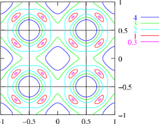
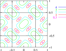
(a)                                     (b)

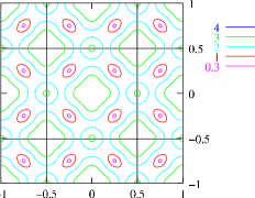
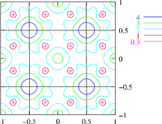
(c)                                     (d)

Figure 1: Contour plot of the spinon dispersion $E_{+}(\boldsymbol{k})$ as a function of $(k_{x}/2\pi,k_{y}/2\pi)$ for the $Z_{2}$-linear spin liquids. (a) is for the Z2A$0013$ state in Eq. (V.2), (b) for the Z2A$zz13$ state in Eq. (V.2), (c) for the Z2A$001n$ state in Eq. (87), (d) for the Z2A$zz1n$ state in Eq. (88).

The spinons are gapless at four isolated points with a linear dispersion for the first four $Z_{2}$ spin liquids Eq. (V.2), Eq. (V.2), Eq. (87), and Eq. (88). (See Fig. 1) Therefore the four ansatz describe symmetric $Z_{2}$-linear spin liquids. The single spinon dispersion for the second $Z_{2}$ spin liquid Z2A$zz13$ is quite interesting. It has the $90^{\circ}$ rotation symmetry around $\boldsymbol{k}=(0,\pi)$ and the parity symmetry about $\boldsymbol{k}=(0,0)$. One very important thing to notice is that the spinon dispersions for the four $Z_{2}$-linear spin liquids, Eq. (V.2), Eq. (V.2), Eq. (87), and Eq. (88) have some qualitative differences between them. Those differences can be used to physically measure quantum orders (see section VII).

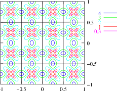
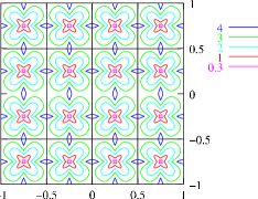
(a)                                     (b)

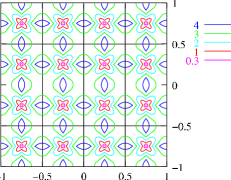
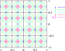
(c)                                     (d)

Figure 2: Contour plot of the spinon dispersion min$(E_{1}(\boldsymbol{k}),E_{2}(\boldsymbol{k}))$ as a function of $(k_{x}/2\pi,k_{y}/2\pi)$ for the $Z_{2}$-linear states. (a) is for the Z2B$0013$ state in Eq. (V.2), (b) for the Z2B$zz13$ state in Eq. (V.2), (c) for the Z2B$001n$ state in Eq. (91), (d) for the Z2B$zz1n$ state in Eq. (92).

Next let us consider the ansatz Z2B$0013$ in Eq. (V.2). The spinon spectrum for ansatz Eq. (V.2) is determined by

$$H= -2\chi\cos(k_{x})\Gamma_{0}-2\eta\cos(k_{x})\Gamma_{2}$$

$$-2\chi\cos(k_{y})\Gamma_{1}+2\eta\cos(k_{y})\Gamma_{3}+\lambda\Gamma_{4}$$ (93)

where $k_{x}\in(0,\pi)$, $k_{y}\in(-\pi,\pi)$ and

$$\Gamma_{0}= \tau^{1}\otimes\tau^{3}, \Gamma_{1}= \tau^{1}\otimes\tau^{1},$$

$$\Gamma_{2}= \tau^{2}\otimes\tau^{3}, \Gamma_{3}= \tau^{2}\otimes\tau^{1},$$

$$\Gamma_{4}= \tau^{1}\otimes\tau^{0}.$$ (94)

assuming $\gamma_{1,2}=\lambda_{2}=0$. The four bands of spinon dispersion have a form $\pm E_{1}(\boldsymbol{k})$, $\pm E_{2}(\boldsymbol{k})$. We find the spinon spectrum vanishes at 8 isolated points near $\boldsymbol{k}=(\pi/2,\pm\pi/2)$. (See Fig. 2a.) Thus the state Z2B$0013$ is a $Z_{2}$-linear spin liquid.

Knowing the translation symmetry of the above $Z_{2}$-linear spin liquid, it seems strange to find that the spinon spectrum is defined only on half of the lattice Brillouin zone. However, this is not inconsistent with translation symmetry since the single spinon excitation is not physical. Only two-spinon excitations correspond to physical excitations and their spectrum should be defined on the full Brillouin zone. Now the problem is that how to obtain two-spinon spectrum defined on the full Brillouin zone from the single-spinon spectrum defined on half of the Brillouin zone. Let $|\boldsymbol{k},1\rangle$ and $|\boldsymbol{k},2\rangle$ be the two eigenstates of single spinon with positive energies $E_{1}(\boldsymbol{k})$ and $E_{2}(\boldsymbol{k})$ (here $k_{x}\in(-\pi/2,\pi/2)$ and $k_{y}\in(-\pi,\pi)$). The translation by $\hat{\boldsymbol{x}}$ (followed by a gauge transformation) change $|\boldsymbol{k},1\rangle$ and $|\boldsymbol{k},2\rangle$ to the other two eigenstates with the same energies:

$$|\boldsymbol{k},1\rangle\to |\boldsymbol{k}+\pi\hat{\boldsymbol{y}},1\rangle$$

$$|\boldsymbol{k},2\rangle\to |\boldsymbol{k}+\pi\hat{\boldsymbol{y}},2\rangle$$ (95)

Now we see that momentum and the energy of two-spinon states $|\boldsymbol{k}_{1},\alpha_{1}\rangle|\boldsymbol{k}_{2},\alpha_{2}\rangle\pm|\boldsymbol{k}_{1}+\pi\hat{\boldsymbol{y}},\alpha_{1}\rangle|\boldsymbol{k}_{2}+\pi\hat{\boldsymbol{y}},\alpha_{2}\rangle$ are given by

$$E_{2spinon}= E_{\alpha_{1}}(\boldsymbol{k}_{1})+E_{\alpha_{2}}(\boldsymbol{k}_{2})$$

$$\boldsymbol{k}= \boldsymbol{k}_{1}+\boldsymbol{k}_{2},\ \ \boldsymbol{k}_{1}+\boldsymbol{k}_{2}+\pi\hat{\boldsymbol{x}}$$ (96)

Eq. (V.2) allows us to construct two-spinon spectrum from single-spinon spectrum.

Now let us consider the ansatz Z2B$zz13$ in Eq. (V.2). The spinon spectrum for ansatz Eq. (V.2) is determined by

$$H= -2\chi\cos(k_{x})\Gamma_{0}-2\eta\cos(k_{x})\Gamma_{2}$$

$$-2\chi\cos(k_{y})\Gamma_{1}+2\eta\cos(k_{y})\Gamma_{3}$$ (97)

$$-2\gamma_{1}\cos(2k_{x}+2k_{y})\Gamma_{4}+2\gamma_{1}\cos(2k_{x}-2k_{y})\Gamma_{4}$$

where $k_{x}\in(0,\pi)$, $k_{y}\in(-\pi,\pi)$ and

$$\Gamma_{0}= \tau^{1}\otimes\tau^{3}, \Gamma_{1}= \tau^{1}\otimes\tau^{1},$$

$$\Gamma_{2}= \tau^{2}\otimes\tau^{3}, \Gamma_{3}= \tau^{2}\otimes\tau^{1},$$

$$\Gamma_{4}= \tau^{1}\otimes\tau^{0}.$$ (98)

We find the spinon spectrum to vanish at 2 isolated points $\boldsymbol{k}=(\pi/2,\pm\pi/2)$. (See Fig. 2b.) The state Z2B$zz13$ is a $Z_{2}$-linear spin liquid.

The spinon spectrum for the ansatz Z2B$001n$ in Eq. (91) is determined by

$$H= -2\chi\cos(k_{x})\Gamma_{0}-2\eta\cos(k_{x})\Gamma_{2}$$

$$-2\chi\cos(k_{y})\Gamma_{1}+2\eta\cos(k_{y})\Gamma_{3}$$

$$+2\lambda(\cos(k_{x}+2k_{y})+\cos(-k_{x}+2k_{y}))\Gamma_{4}$$

$$-2\lambda(\cos(2k_{x}+k_{y})+\cos(2k_{x}-k_{y}))\Gamma_{5}$$ (99)

where $k_{x}\in(0,\pi)$, $k_{y}\in(-\pi,\pi)$ and

$$\Gamma_{0}= \tau^{1}\otimes\tau^{3}, \Gamma_{1}= \tau^{1}\otimes\tau^{1},$$

$$\Gamma_{2}= \tau^{2}\otimes\tau^{3}, \Gamma_{3}= \tau^{2}\otimes\tau^{1},$$

$$\Gamma_{4}= \tau^{3}\otimes\tau^{3}, \Gamma_{5}= \tau^{3}\otimes\tau^{1}.$$ (100)

The spinon spectrum vanishes at 2 isolated points $\boldsymbol{k}=(\pi/2,\pm\pi/2)$. (See Fig. 2c.) The state Z2B$001n$ is also a $Z_{2}$-linear spin liquid.

The spinon spectrum for the ansatz Z2B$zz1n$ in Eq. (92) can be obtained from

$$H= -2\chi\cos(k_{x})\Gamma_{0}-2\eta\cos(k_{x})\Gamma_{2}$$

$$-2\chi\cos(k_{y})\Gamma_{1}+2\eta\cos(k_{y})\Gamma_{3}$$

$$+2\lambda(\cos(k_{x}+2k_{y})-\cos(-k_{x}+2k_{y}))\Gamma_{4}$$

$$-2\lambda(\cos(2k_{x}+k_{y})-\cos(2k_{x}-k_{y}))\Gamma_{5}$$ (101)

where $k_{x}\in(0,\pi)$, $k_{y}\in(-\pi,\pi)$ and

$$\Gamma_{0}= \tau^{1}\otimes\tau^{3}, \Gamma_{1}= \tau^{1}\otimes\tau^{1},$$

$$\Gamma_{2}= \tau^{2}\otimes\tau^{3}, \Gamma_{3}= \tau^{2}\otimes\tau^{1},$$

$$\Gamma_{4}= \tau^{3}\otimes\tau^{3}, \Gamma_{5}= \tau^{3}\otimes\tau^{1}.$$ (102)

We have also assumed that $\chi_{1}=\eta_{1}=0$. The spinon spectrum vanishes at 2 isolated points $\boldsymbol{k}=(\pi/2,\pm\pi/2)$. (See Fig. 2d.) The state Z2B$zz1n$ is again a $Z_{2}$-linear spin liquid.

V.3 Symmetric spin liquids around the $SU(2)$-gapless spin liquid SU2A$n0$

There are many types of symmetric ansatz in the neighborhood of the $SU(2)$-gapless state Eq. (III). Let us first consider the 12 classes of symmetric $U(1)$ spin liquids around the $SU(2)$-gapless state Eq. (B.4) – Eq. (B.4). Here we just present the simple cases where $u_{\boldsymbol{i}\boldsymbol{j}}$ are non-zero only for links with length $\leq 2$. Among the 12 classes of symmetric ansatz, We find that 5 classes actually give us the $SU(2)$-gapless spin liquid when the link length is $\leq 2$. The other 7 symmetric $U(1)$ spin liquids are given bellow.

From Eq. (B.4) we get

$$u_{\boldsymbol{i},\boldsymbol{i}+\hat{\boldsymbol{x}}}= \chi\tau^{1}-\eta\tau^{2} u_{\boldsymbol{i},\boldsymbol{i}+\hat{\boldsymbol{y}}}= \chi\tau^{1}+\eta\tau^{2}$$

$$a^{1,2,3}_{0}= 0$$

$$G_{x}= G_{y}=\tau^{0}, G_{P_{x}}= G_{P_{y}}=\tau^{0},$$

$$G_{P_{xy}}= i\tau^{1}, G_{T}= (-)^{\boldsymbol{i}}\tau^{0}$$ (103)

In the above, we have also listed the gauge transformations $G_{x,y}$, $G_{P_{x},P_{y},P_{xy}}$ and $G_{T}$ associated translation, parity and time reversal transformations. Those gauge transformations define the PSG that characterizes the $U(1)$ spin liquid. In section IV.3, we have introduced a notation U1C$n01n$ to label the PSG and its associated ansatz. In the following, we will list ansatz together with their labels and the associated gauge transformations.

From Eq. (B.4) we get U1C$n00x$ state

$$u_{\boldsymbol{i},\boldsymbol{i}+\hat{\boldsymbol{x}}}= \chi\tau^{1} u_{\boldsymbol{i},\boldsymbol{i}+\hat{\boldsymbol{y}}}= \chi\tau^{1}$$

$$u_{\boldsymbol{i},\boldsymbol{i}+\hat{\boldsymbol{x}}+\hat{\boldsymbol{y}}}= \eta_{1}\tau^{3} u_{\boldsymbol{i},\boldsymbol{i}-\hat{\boldsymbol{x}}+\hat{\boldsymbol{y}}}= \eta_{1}\tau^{3}$$

$$u_{\boldsymbol{i},\boldsymbol{i}+2\hat{\boldsymbol{x}}}= \eta_{2}\tau^{3} u_{\boldsymbol{i},\boldsymbol{i}+2\hat{\boldsymbol{y}}}= \eta_{2}\tau^{3}$$

$$a^{3}_{0}= \eta_{3}, a^{1,2}_{0}= 0$$

$$G_{x}= G_{y}=\tau^{0}, G_{P_{x}}= G_{P_{y}}=\tau^{0},$$

$$G_{P_{xy}}= \tau^{0}, G_{T}= i\tau^{2}$$ (104)

U1C$n01x$ state

$$u_{\boldsymbol{i},\boldsymbol{i}+\hat{\boldsymbol{x}}}= \chi\tau^{1} u_{\boldsymbol{i},\boldsymbol{i}+\hat{\boldsymbol{y}}}= \chi\tau^{1}$$

$$u_{\boldsymbol{i},\boldsymbol{i}+2\hat{\boldsymbol{x}}}= -\eta_{2}\tau^{3} u_{\boldsymbol{i},\boldsymbol{i}+2\hat{\boldsymbol{y}}}= \eta_{2}\tau^{3}$$

$$a^{1,2,3}_{0}= 0$$

$$G_{x}= G_{y}=\tau^{0}, G_{P_{x}}= G_{P_{y}}=\tau^{0},$$

$$G_{P_{xy}}= i\tau^{1}, G_{T}= i\tau^{2}$$ (105)

and U1C$x10x$ state

$$u_{\boldsymbol{i},\boldsymbol{i}+\hat{\boldsymbol{x}}}= \chi\tau^{1} u_{\boldsymbol{i},\boldsymbol{i}+\hat{\boldsymbol{y}}}= \chi\tau^{1}$$

$$u_{\boldsymbol{i},\boldsymbol{i}+\hat{\boldsymbol{x}}+\hat{\boldsymbol{y}}}= -\eta\tau^{3} u_{\boldsymbol{i},\boldsymbol{i}-\hat{\boldsymbol{x}}+\hat{\boldsymbol{y}}}= \eta\tau^{3}$$

$$a^{1,2,3}_{0}= 0$$

$$G_{x}= G_{y}=\tau^{0}, G_{P_{x}}= G_{P_{y}}=i\tau^{1},$$

$$G_{P_{xy}}= \tau^{0}, G_{T}= i\tau^{2}$$ (106)

From Eq. (B.4) we get U1A$0001$ state

$$u_{\boldsymbol{i},\boldsymbol{i}+\hat{\boldsymbol{x}}}= i\chi\tau^{0} u_{\boldsymbol{i},\boldsymbol{i}+\hat{\boldsymbol{y}}}= i\chi\tau^{0}$$

$$u_{\boldsymbol{i},\boldsymbol{i}+\hat{\boldsymbol{x}}+\hat{\boldsymbol{y}}}= -\eta_{1}\tau^{3} u_{\boldsymbol{i},\boldsymbol{i}-\hat{\boldsymbol{x}}+\hat{\boldsymbol{y}}}= \eta_{1}\tau^{3}$$

$$u_{\boldsymbol{i},\boldsymbol{i}+2\hat{\boldsymbol{x}}}= \eta_{2}\tau^{3} u_{\boldsymbol{i},\boldsymbol{i}+2\hat{\boldsymbol{y}}}= \eta_{2}\tau^{3}$$

$$a^{1,2,3}_{0}= 0$$

$$G_{x}= G_{y}=\tau^{0}, (-)^{i_{x}}G_{P_{x}}= (-)^{i_{x}}G_{P_{y}}=\tau^{0},$$

$$G_{P_{xy}}= \tau^{0}, G_{T}= i(-)^{\boldsymbol{i}}\tau^{1}$$ (107)

and U1A$0011$ state

$$u_{\boldsymbol{i},\boldsymbol{i}+\hat{\boldsymbol{x}}}= i\chi\tau^{0} u_{\boldsymbol{i},\boldsymbol{i}+\hat{\boldsymbol{y}}}= i\chi\tau^{0}$$

$$u_{\boldsymbol{i},\boldsymbol{i}+2\hat{\boldsymbol{x}}}= -\eta_{2}\tau^{3} u_{\boldsymbol{i},\boldsymbol{i}+2\hat{\boldsymbol{y}}}= \eta_{2}\tau^{3}$$

$$a^{1,2,3}_{0}= 0$$

$$G_{x}= G_{y}=\tau^{0}, (-)^{i_{x}}G_{P_{x}}= (-)^{i_{x}}G_{P_{y}}=\tau^{0},$$

$$G_{P_{xy}}= i\tau^{1}, G_{T}= i(-)^{\boldsymbol{i}}\tau^{1}$$ (108)

From Eq. (B.4) we get, for $G_{P_{xy}}=g_{3}(\theta_{pxy})$, U1A$x10x$ state

$$u_{\boldsymbol{i},\boldsymbol{i}+\hat{\boldsymbol{x}}}= i\chi\tau^{0} u_{\boldsymbol{i},\boldsymbol{i}+\hat{\boldsymbol{y}}}= i\chi\tau^{0}$$

$$u_{\boldsymbol{i},\boldsymbol{i}+\hat{\boldsymbol{x}}+\hat{\boldsymbol{y}}}= \eta\tau^{3} u_{\boldsymbol{i},\boldsymbol{i}-\hat{\boldsymbol{x}}+\hat{\boldsymbol{y}}}= \eta\tau^{3}$$

$$a^{1,2,3}_{0}= 0$$

$$G_{x}= G_{y}=\tau^{0}, (-)^{i_{x}}G_{P_{x}}= (-)^{i_{x}}G_{P_{y}}=i\tau^{1},$$

$$G_{P_{xy}}= \tau^{0}, G_{T}= i(-)^{\boldsymbol{i}}\tau^{1}$$ (109)

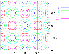
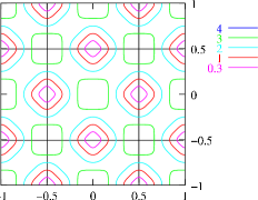
(a)                                     (b)

Figure 3: Contour plot of the spinon dispersion $E_{+}(\boldsymbol{k})$ as a function of $(k_{x}/2\pi,k_{y}/2\pi)$ for (a) the $U(1)$-linear state U1C$n00x$ in Eq. (V.3), and (b) the $U(1)$-quadratic state U1C$x10x$ in Eq. (V.3). In the $U(1)$-quadratic state, the spinon energy vanishes as $\Delta\boldsymbol{k}^{2}$ near two points $\boldsymbol{k}=(\pi,0),(0,\pi)$.

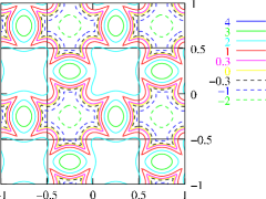
(a)                                     (b)

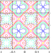
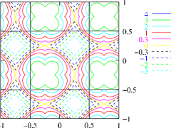
(c)                                     (d)

Figure 4: Contour plot of the spinon dispersion $E_{+}(\boldsymbol{k})$ as a function of $(k_{x}/2\pi,k_{y}/2\pi)$ for the $U(1)$-gapless states. (a) is for the U1C$n01x$ state Eq. (V.3), (b) for the U1A$0001$ state Eq. (V.3), (c) for the U1A$0011$ state Eq. (V.3), and (d) for the U1A$x10x$ state Eq. (V.3).

Eq. (V.3) is the U1C$n01n$ $U(1)$-linear state (the staggered flux state) studied in the last section. After examining the spinon dispersion, we find that the U1C$n00x$ state in Eq. (V.3) can be a $U(1)$-linear or a $U(1)$-gapped state depending on the value of $a^{3}_{0}$. If it is a $U(1)$-linear state, it will have 8 isolated Fermi points (see Fig. 3a). The U1C$n01x$ state in Eq. (V.3) is a $U(1)$-gapless state (see Fig. 4a). The U1C$x10x$ state in Eq. (V.3) has two Fermi points at $\boldsymbol{k}_{1}=(\pi,0)$ and $\boldsymbol{k}_{2}=(0,\pi)$. (see Fig. 3b). However, the spinon energy has a form $E(\boldsymbol{k})\propto(\boldsymbol{k}-\boldsymbol{k}_{1,2})^{2}$ near $\boldsymbol{k}_{1}$ and $\boldsymbol{k}_{2}$. Thus we call the U1C$x10x$ spin liquid Eq. (V.3) a $U(1)$-quadratic state. The U1A$0001$ state in Eq. (V.3), the U1A$0011$ state in Eq. (V.3), and the U1A$x10x$ state in Eq. (V.3) are $U(1)$-gapless states (see Fig. 4). Again the spinon dispersions for the $U(1)$ spin liquids have some qualitative differences between each other, which can be used to detect different quantum orders in those $U(1)$ spin liquids.

We next consider the 52 classes of symmetric $Z_{2}$ spin liquids around the $SU(2)$-gapless state Eq. (B.4) – Eq. (452). Here we just present the simplest case where $u_{\boldsymbol{i}\boldsymbol{j}}$ are non-zero only for links with length $\leq 1$. We find that 48 out of 52 classes of ansatz describe $U(1)$ or $SU(2)$ spin liquids when the link’s length is $\leq 1$. In the following we discuss the 4 remaining $Z_{2}$ ansatz.

We obtain one $Z_{2}$ spin liquid Z2A$x2(12)n$ from Eq. (B.4). It is described by Eq. (III). From Eq. (444), we obtain a $Z_{2}$ spin liquid Z2A$0013$. It is described by Eq. (V.2) or Eq. (III). From Eq. (B.4), we obtain a $Z_{2}$ spin liquid Z2B$y1(12)n$ (note Z2B$y1(12)n$ is gauge equivalent to Z2B$x2(12)n$ ):

$$u_{\boldsymbol{i},\boldsymbol{i}+\hat{\boldsymbol{x}}}= i\chi\tau^{0}+\eta_{1}\tau^{1}$$

$$u_{\boldsymbol{i},\boldsymbol{i}+\hat{\boldsymbol{y}}}= (-)^{i_{x}}(i\chi\tau^{0}+\eta_{1}\tau^{2})$$

$$a^{1,2,3}_{0}= 0$$ (110)

From Eq. (452), we obtain a $Z_{2}$ spin liquid Z2B$0013$, which is described by Eq. (V.2).

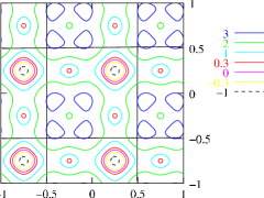
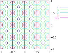
(a)                                     (b)

Figure 5: Contour plot of the spinon dispersion $E_{+}(\boldsymbol{k})$ as a function of $(k_{x}/2\pi,k_{y}/2\pi)$ for the $Z_{2}$ spin liquids. (a) is for $Z_{2}$-gapless state Z2A$x2(12)n$ in Eq. (III), and (b) is for $Z_{2}$-quadratic state Z2B$x2(12)n$ in Eq. (V.3). Despite the lack of rotation and parity symmetries in the single spinon dispersion in (a), the two-spinon spectrum does have those symmetries.

The ansatz Z2B$x2(12)n$ in Eq. (V.3) is a new $Z_{2}$ spin liquid. The spinon spectrum for ansatz Eq. (V.3) is determined by

$$H= -2\chi\sin(k_{x})\Gamma_{0}+2\eta\cos(k_{x})\Gamma_{2}$$

$$-2\chi\sin(k_{y})\Gamma_{1}+2\eta\cos(k_{y})\Gamma_{3}$$ (111)

where $k_{x}\in(-\pi/2,\pi/2)$, $k_{y}\in(-\pi,\pi)$ and

$$\Gamma_{0}= \tau^{0}\otimes\tau^{3}, \Gamma_{2}= \tau^{1}\otimes\tau^{3},$$

$$\Gamma_{1}= \tau^{0}\otimes\tau^{1}, \Gamma_{3}= \tau^{2}\otimes\tau^{1}.$$ (112)

The spinon spectrum can be calculated exactly and its four branches take a form $\pm E_{1}(\boldsymbol{k})$ and $\pm E_{2}(\boldsymbol{k})$. The spinon energy vanishes at two isolated points $\boldsymbol{k}=(0,0),(0,\pi)$. Near $\boldsymbol{k}=0$ the low energy spectrum is given by (see Fig. 5b)

$$E=\pm\eta^{-1}\sqrt{(\chi^{2}+\eta^{2})^{2}(k_{x}^{2}-k_{y}^{2})^{2}+4\chi^{4}k_{x}^{2}k_{y}^{2}}$$ (113)

It is interesting to see that the energy does not vanish linearly as $\boldsymbol{k}\to 0$, instead it vanishes like $\boldsymbol{k}^{2}$.

We find that the loop operators for the following loops $\boldsymbol{i}\to\boldsymbol{i}+\hat{\boldsymbol{x}}\to\boldsymbol{i}+\hat{\boldsymbol{x}}+\hat{\boldsymbol{y}}\to\boldsymbol{i}+\hat{\boldsymbol{y}}\to\boldsymbol{i}$ and $\boldsymbol{i}\to\boldsymbol{i}+\hat{\boldsymbol{y}}\to\boldsymbol{i}-\hat{\boldsymbol{x}}+\hat{\boldsymbol{y}}\to\boldsymbol{i}-\hat{\boldsymbol{x}}\to\boldsymbol{i}$ do not commute as long as both $\chi$ and $\eta$ are non-zero. Thus the spin liquid described by Eq. (V.3) indeed has a $Z_{2}$ gauge structure. We will call such a state $Z_{2}$-quadratic spin liquid to stress the $E\propto\boldsymbol{k}^{2}$ dispersion. Such a state cannot be constructed from translation invariant ansatz, and it is the reason why we missed this state in the last section. The two-spinon spectrum is still related to the one-spinon spectrum through Eq. (V.2).

V.4 Symmetric spin liquids around the $SU(2)$-linear spin liquid SU2B$n0$

Last, we consider symmetric states in the neighborhood of the $SU(2)$-linear state Eq. (III). The PSG’s for those symmetric states can be obtained through the mapping Eq. (A.3) from the PSG’s of symmetric spin liquids around the $SU(2)$-gapless spin liquid. Here we will only consider the 12 classes of symmetric $U(1)$ spin liquids around the $SU(2)$-linear state given by Eq. (461) – Eq. (466). We will just present the simple cases where $u_{\boldsymbol{i}\boldsymbol{j}}$ are non-zero only for links with length $\leq 2$. We find that 7 of 12 classes of ansatz actually give us $SU(2)$-gapless spin liquids when the link length is $\leq 2$. Thus we only obtain the following 5 symmetric $U(1)$ spin liquids.

From Eq. (B.5) we get U1C$n01n$ ansatz

$$u_{\boldsymbol{i},\boldsymbol{i}+\hat{\boldsymbol{x}}}= \chi\tau^{1}-\eta\tau^{2} u_{\boldsymbol{i},\boldsymbol{i}+\hat{\boldsymbol{y}}}= \chi\tau^{1}+\eta\tau^{2}$$

$$a^{1,2,3}_{0}= 0$$

$$G_{x}= G_{y}=\tau^{0}, G_{P_{x}}= G_{P_{y}}=\tau^{0},$$

$$G_{P_{xy}}= i\tau^{1}, G_{T}= (-)^{\boldsymbol{i}}\tau^{0}$$ (114)

which has the same quantum order as in the $U(1)$-linear state Eq. (III) (the staggered-flux state).

From Eq. (B.5) we get U1C$n0x1$ ansatz

$$u_{\boldsymbol{i},\boldsymbol{i}+\hat{\boldsymbol{x}}}= \chi\tau^{2} u_{\boldsymbol{i},\boldsymbol{i}+\hat{\boldsymbol{y}}}= \chi\tau^{1}$$

$$u_{\boldsymbol{i},\boldsymbol{i}+2\hat{\boldsymbol{x}}}= -\eta\tau^{3} u_{\boldsymbol{i},\boldsymbol{i}+2\hat{\boldsymbol{y}}}= \eta\tau^{3}$$

$$a^{1,2,3}_{0}= 0$$

$$G_{x}= G_{y}=\tau^{0}, G_{P_{x}}= G_{P_{y}}=\tau^{0},$$

$$G_{P_{xy}}= i\tau^{12}, G_{T}= (-)^{i_{y}}i\tau^{1}$$ (115)

and U1C$n0n1$ ansatz

$$u_{\boldsymbol{i},\boldsymbol{i}+\hat{\boldsymbol{x}}}= \chi\tau^{2},\ \ \ \ u_{\boldsymbol{i},\boldsymbol{i}+\hat{\boldsymbol{y}}}=\chi\tau^{1}$$

$$u_{\boldsymbol{i},\boldsymbol{i}+2\hat{\boldsymbol{x}}}= \eta\tau^{3},\ \ \ \ u_{\boldsymbol{i},\boldsymbol{i}+2\hat{\boldsymbol{y}}}=\eta\tau^{3}$$

$$a^{3}_{0}= \eta_{1},\ \ \ \ a^{1,2}_{0}=0$$

$$G_{x}= G_{y}=\tau^{0},\ \ \ \ G_{T}=(-)^{i_{y}}i\tau^{1}$$

$$G_{P_{x}}= G_{P_{y}}=\tau^{0},$$

$$G_{P_{xy}}= (-)^{i_{x}i_{y}}g_{3}(((-)^{i_{x}}-(-)^{i_{y}})\pi/4).$$ (116)

From Eq. (465) we get U1B$0001$ ansatz

$$u_{\boldsymbol{i},\boldsymbol{i}+\hat{\boldsymbol{x}}}= i\chi\tau^{0} u_{\boldsymbol{i},\boldsymbol{i}+\hat{\boldsymbol{y}}}= i(-)^{i_{x}}\chi\tau^{0}$$

$$u_{\boldsymbol{i},\boldsymbol{i}+2\hat{\boldsymbol{x}}}= \eta\tau^{3} u_{\boldsymbol{i},\boldsymbol{i}+2\hat{\boldsymbol{y}}}= \eta\tau^{3}$$

$$a^{3}_{0}= \eta_{1}, a^{1,2}_{0}= 0$$

$$(-)^{i_{y}}G_{x}= G_{y}=\tau^{0}, (-)^{i_{x}}G_{P_{x}}= (-)^{i_{x}}G_{P_{y}}=\tau^{0},$$

$$G_{P_{xy}}= (-)^{i_{x}i_{y}}\tau^{0}, G_{T}= i(-)^{\boldsymbol{i}}\tau^{1}$$ (117)

and U1B$0011$ ansatz

$$u_{\boldsymbol{i},\boldsymbol{i}+\hat{\boldsymbol{x}}}= i\chi\tau^{0} u_{\boldsymbol{i},\boldsymbol{i}+\hat{\boldsymbol{y}}}= i(-)^{i_{x}}\chi\tau^{0}$$

$$u_{\boldsymbol{i},\boldsymbol{i}+2\hat{\boldsymbol{x}}}= -\eta\tau^{3} u_{\boldsymbol{i},\boldsymbol{i}+2\hat{\boldsymbol{y}}}= \eta\tau^{3}$$

$$a^{1,2,3}_{0}= 0$$

$$(-)^{i_{y}}G_{x}= G_{y}=\tau^{0}, (-)^{i_{x}}G_{P_{x}}= (-)^{i_{x}}G_{P_{y}}=\tau^{0},$$

$$G_{P_{xy}}= i(-)^{i_{x}i_{y}}\tau^{1}, G_{T}= i(-)^{\boldsymbol{i}}\tau^{1}$$ (118)

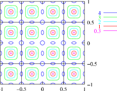
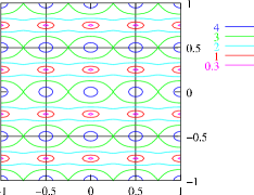
(a)                                     (b)

Figure 6: Contour plot of the spinon dispersion $E_{+}(\boldsymbol{k})$ as a function of $(k_{x}/2\pi,k_{y}/2\pi)$ for (a) the $U(1)$-linear state U1C$n0x1$ in Eq. (V.4) and (b) the $U(1)$-linear state Eq. (VI).

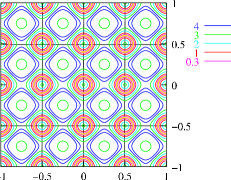
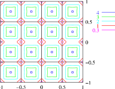
(a)                                     (b)

Figure 7: Contour plot of the spinon dispersion min$(E_{1}(\boldsymbol{k}),E_{2}(\boldsymbol{k}))$ as a function of $(k_{x}/2\pi,k_{y}/2\pi)$ for the $U(1)$ spin liquid states. (a) is for the $U(1)$-gapless state U1B$0001$ in Eq. (V.4) and (b) is for the $U(1)$-linear state U1B$0011$ in Eq. (V.4).

Now let us discuss spinon dispersions in the above $U(1)$ spin liquids. The spinon in the U1C$n0x1$ state Eq. (V.4) has 4 linear nodes at $(\pm\pi/2,\pm\pi/2)$. Thus U1C$n0x1$ state is a $U(1)$-linear spin liquid. The U1C$n0n1$ state Eq. (V.4) has fully gapped spinons and is a $U(1)$-gapped spin liquid.

The four spinon bands in the U1B$0001$ state Eq. (V.4) are given by (see Fig. 7a)

$$\pm 2\chi\sqrt{\sin^{2}(k_{x})+\sin^{2}(k_{y})}\pm(2\eta\cos(2k_{x})+2\eta\cos(2k_{y})+\eta_{1})$$ (119)

We find that the U1B$0001$ state is a $U(1)$-gapless spin liquid. The four spinon bands in the U1B$0011$ state Eq. (V.4) are given by (see Fig. 7b)

$$\pm 2\chi\sqrt{\sin^{2}(k_{x})+\sin^{2}(k_{y})}\pm 2\eta(\cos(2k_{x})-\cos(2k_{y}))$$ (120)

Hence, the U1B$0011$ state is a $U(1)$-linear spin liquid.

To summarize we list all the spin liquids discussed so far in the following table:

$Z_{2}$-gapped Z2A$xx0z$ $Z_{2}$-linear Z2A$0013$, Z2A$zz13$, Z2A$001n$ Z2A$zz1n$, Z2B$0013$, Z2B$zz13$ Z2B$001n$, Z2B$zz1n$ $Z_{2}$-quadratic Z2B$x2(12)n$ $Z_{2}$-gapless Z2A$x2(12)n$ $U(1)$-gapped U1C$n00x$ $U(1)$-linear U1B$0011$, U1C$n00x$, U1C$n01n$ U1C$n0x1$ $U(1)$-quadratic U1C$x10x$ $U(1)$-gapless U1A$0001$, U1A$0011$, U1A$x10x$ U1B$0001$, U1C$n01x$ $SU(2)$-linear SU2B$n0$ $SU(2)$-gapless SU2A$n0$

VI Mean-field phase diagram of $J_{1}$-$J_{2}$ model

To see which of the $Z_{2}$, $U(1)$, and $SU(2)$ spin liquids discussed in the last section have low ground energies and may appear in real high $T_{c}$ superconductors, we calculate the mean-field energy of a large class of translation invariant ansatz. In Fig. 8, we present the resulting mean-field phase diagram for a $J_{1}$-$J_{2}$ spin system. Here $J_{1}$ is the nearest-neighbor spin coupling and $J_{2}$ is the next-nearest-neighbor spin coupling. We have fixed $J_{1}+J_{2}=1$. The $y$-axis is the mean-field energy per site (multiplied by a factor $8/3$). The phase (A) is the $\pi$-flux state (the SU2B$n0$ $SU(2)$-linear state) Eq. (III). The phase (B) is a state with two independent uniform RVB states on the diagonal links. It has $SU(2)\times SU(2)$ gauge fluctuations at low energies and will be called an $SU(2)\times SU(2)$-gapless state. Its ansatz is given by

$$u_{\boldsymbol{i},\boldsymbol{i}+\hat{\boldsymbol{x}}+\hat{\boldsymbol{y}}}= \chi\tau^{3}$$

$$u_{\boldsymbol{i},\boldsymbol{i}+\hat{\boldsymbol{x}}-\hat{\boldsymbol{y}}}= \chi\tau^{3}$$

$$a^{l}_{0}= 0$$ (121)

The phase (C) is a state with two independent $\pi$-flux states on the diagonal links. It has $SU(2)\times SU(2)$ gauge fluctuations at low energies and will be called an $SU(2)\times SU(2)$-linear state. Its ansatz is given by

$$u_{\boldsymbol{i},\boldsymbol{i}+\hat{\boldsymbol{x}}+\hat{\boldsymbol{y}}}= \chi(\tau^{3}+\tau^{1})$$

$$u_{\boldsymbol{i},\boldsymbol{i}+\hat{\boldsymbol{x}}-\hat{\boldsymbol{y}}}= \chi(\tau^{3}-\tau^{1})$$

$$a^{l}_{0}= 0$$ (122)

The phase (D) is the chiral spin state Eq. (III). The phase (E) is described by an ansatz

$$u_{\boldsymbol{i},\boldsymbol{i}+\hat{\boldsymbol{x}}+\hat{\boldsymbol{y}}}= \chi_{1}\tau^{1}+\chi_{2}\tau^{2}$$

$$u_{\boldsymbol{i},\boldsymbol{i}+\hat{\boldsymbol{x}}-\hat{\boldsymbol{y}}}= \chi_{1}\tau^{1}-\chi_{2}\tau^{2}$$

$$u_{\boldsymbol{i},\boldsymbol{i}+\hat{\boldsymbol{y}}}= \eta\tau^{3}$$

$$a^{l}_{0}= 0$$ (123)

which break the $90^{\circ}$ rotation symmetry and is a $U(1)$-linear state (see Fig. 6b). The phase (F) is described by the U1C$n00x$ ansatz in Eq. (V.3). The U1C$n00x$ state can be a $U(1)$-linear or a $U(1)$-gapped state. The state for phase (F) turns out to be a $U(1)$-gapped state. The phase (G) is described by the Z2A$zz13$ ansatz in Eq. (V.2) which is a $Z_{2}$-linear state. The phase (H) is described by the Z2A$0013$ ansatz in Eq. (V.2) and is also a $Z_{2}$-linear state. The phase (I) is the uniform RVB state (the $SU(2)$-gapless state SU2A$n0$ Eq. (III)).

From Fig. 8, we see continuous phase transitions (at mean-field level) between the following pairs of phases: (A,D), (A,G), (B,G), (C,E), and (B,H). The three continuous transitions (B,G), (B,H) and (A,G) do not change any symmetries. We also note that the $SU(2)$ gauge structure in the phase (A) breaks down to $Z_{2}$ in the continuous transition from the phase (A) to the phase (G). The $SU(2)\times SU(2)$ gauge structure in the phase (B) breaks down to $Z_{2}$ in the two transitions (B,G) and (B,H).

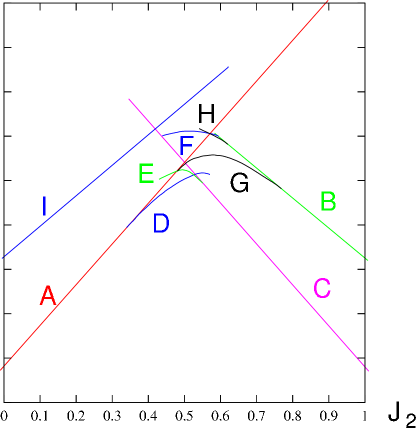
Figure 8: The mean-field energies for various phases in a $J_{1}$-$J_{2}$ spin system. (A) the $\pi$-flux state (the $SU(2)$-linear state SU2B$n0$). (B) the $SU(2)\times SU(2)$-gapless state in Eq. (VI). (C) the $SU(2)\times SU(2)$-linear state in Eq. (VI). (D) the chiral spin state (an $SU(2)$-gapped state). (E) the $U(1)$-linear state Eq. (VI) which breaks $90^{\circ}$ rotation symmetry. (F) the $U(1)$-gapped state U1C$n00x$ in Eq. (V.3). (G) the $Z_{2}$-linear state Z2A$zz13$ in Eq. (V.2). (H) the $Z_{2}$-linear state Z2A$0013$ in Eq. (V.2). (I) the uniform RVB state (the $SU(2)$-gapless state SU2A$n0$).

VII Physical measurements of quantum orders

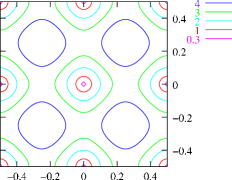
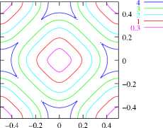
(a)                                     (b)

Figure 9: Contour plot of the dispersion for spin-1 excitation, $E_{2s}(\boldsymbol{k})$, as a function of $(k_{x}/2\pi,k_{y}/2\pi)$ for (a) the $SU(2)$-linear spin liquid SU2B$n0$ in Eq. (III) (the $\pi$-flux phase) and (b) the $U(1)$-quadratic spin liquid U1C$x10x$ in Eq. (V.3).

After characterizing the quantum orders using PSG mathematically, we would like to ask how to measure quantum orders in experiments. The quantum orders in gapped states are related to the topological orders. The measurement of topological orders are discussed in LABEL:Wrig,Wtoprev,SF0192. The quantum order in a state with gapless excitations can be measured, in general, by the dynamical properties of gapless excitation. However, not all dynamical properties are universal. Thus we need to identify the universal properties of gapless excitations, before using them to characterize and measure quantum orders. The PSG characterization of quantum orders allows us obtain those universal properties. We simply need to identify the common properties of gapless excitations that are shared by all the ansatz with the same PSG.

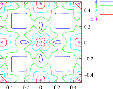
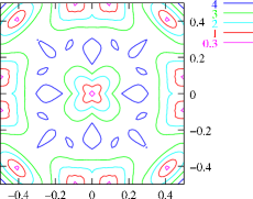
(a)                                     (b)

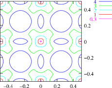
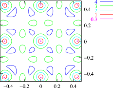
(c)                                     (d)

Figure 10: Contour plot of $E_{2s}(\boldsymbol{k})$ as a function of $(k_{x}/2\pi,k_{y}/2\pi)$ for the $Z_{2}$-linear spin liquids. (a) is for the Z2A$0013$ state in Eq. (V.2), (b) for the Z2A$zz13$ state in Eq. (V.2), (c) for the Z2A$001n$ state in Eq. (87), (d) for the Z2A$zz1n$ state in Eq. (88).

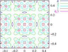
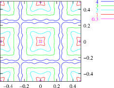
(a)                                     (b)

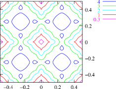
(c)                                     (d)

Figure 11: Contour plot of $E_{2s}(\boldsymbol{k})$ as a function of $(k_{x}/2\pi,k_{y}/2\pi)$ for the $Z_{2}$-linear spin liquids. (a) is for the Z2B$0013$ state in Eq. (V.2), (b) for the Z2B$zz13$ state in Eq. (V.2), (c) for the Z2B$001n$ state in Eq. (91), (d) for the Z2B$zz1n$ state in Eq. (92).

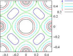
(a)                                     (b)

Figure 12: Contour plot of $E_{2s}(\boldsymbol{k})$ as a function of $(k_{x}/2\pi,k_{y}/2\pi)$ for (a) the $Z_{2}$-gapless state Z2A$x2(12)n$ in Eq. (III), and (b) the $Z_{2}$-quadratic state Z2B$x2(12)n$ in Eq. (V.3).

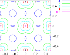
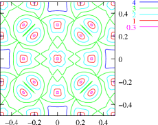
(a)                                     (b)

Figure 13: Contour plot of $E_{2s}(\boldsymbol{k})$ as a function of $(k_{x}/2\pi,k_{y}/2\pi)$ for two $U(1)$-linear spin liquids. (a) is for the U1C$n01n$ state Eq. (III) (the staggered flux phase), and (b) for the U1C$n00x$ state Eq. (V.3) in the gapless phase.

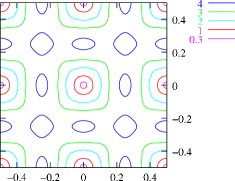
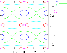
(a)                                     (b)

Figure 14: Contour plot of the two-spinon dispersion $E_{2s}(\boldsymbol{k})$ as a function of $(k_{x}/2\pi,k_{y}/2\pi)$ for (a) the $U(1)$-linear spin liquid state U1C$n0x1$ in Eq. (V.4) and (b) the $U(1)$-linear spin liquid Eq. (VI).

To demonstrate the above idea, we would like to study the spectrum of two-spinon excitations. We note that spinons can only be created in pairs. Thus the one-spinon spectrum is not physical. We also note that the two-spinon spectrum include spin-1 excitations which can be measured in experiments. At a given momentum, the two-spinon spectrum is distributed in one or several ranges of energy. Let $E_{2s}(\boldsymbol{k})$ be the lower edge of the two-spinon spectrum at momentum $\boldsymbol{k}$. In the mean-field theory, the two-spinon spectrum can be constructed from the one-spinon dispersion

$$E_{\text{2-spinon}}(\boldsymbol{k})=E_{\text{1-spinon}}(\boldsymbol{q})+E_{\text{1-spinon}}(\boldsymbol{k}-\boldsymbol{q})$$ (124)

In Fig. 9 – 15 we present mean-field $E_{2s}$ for some simple spin liquids. If the mean-field state is stable against the gauge fluctuations, we expect the mean-field $E_{2s}$ should qualitatively agrees with the real $E_{2s}$.

Among our examples, there are eight $Z_{2}$-linear spin liquids (see Fig. 10 and Fig. 11). We see that some of those eight different $Z_{2}$-linear spin liquids (or eight different quantum orders) have different number of gapless points. The gapless points of some spin liquids are pinned at position $\boldsymbol{k}=(\pi,\pi)$ and/or $\boldsymbol{k}=(\pi,0),(0,\pi)$. By measuring the low energy spin excitations (say using neutron scattering), we can distinguish those $Z_{2}$ spin liquids. We note that all the two-spinon spectra have rotation and parity symmetries around $\boldsymbol{k}=0$. This is expected. Since the two-spinon spectra are physical, they should have all the symmetries the spin liquids have.

We also have four $U(1)$-linear spin liquids. Some of them can be distinguished by their different numbers of gapless points. It is interesting to note that all the $U(1)$ spin liquids discussed here have a gapless point in the two-spinon spectrum pinned at position $\boldsymbol{k}=(\pi,\pi)$. The $U(1)$-linear spin liquids are also different from the $Z_{2}$-linear spin liquids in that the spin-spin correlations have different decay exponents once the $U(1)$ gauge fluctuations are included. We also see that $E_{2s}$ has a quadratic form $E_{2s}\propto\boldsymbol{k}^{2}$ for the $U(1)$-quadratic spin liquid. $E_{2s}$ vanishes in two finite regions in $\boldsymbol{k}$-space for the $Z_{2}$-gapless spin liquids.

Neutron scattering experiments probe the two-spinon sector. Thus low energy neutron scattering allows us to measure quantum orders in high $T_{c}$ superconductors.

Let us discuss the $U(1)$ linear state U1C$n01n$ (the staggered-flux state) in more detail. The U1C$n01n$ state is proposed to describe the pseudo-gap metallic state in underdoped high $T_{c}$ superconductors.WLsu2 ; RWspec The U1C$n01n$ state naturally explains the spin pseudo-gap in the underdoped metallic state. As an algebraic spin liquid, the U1C$n01n$ state also explain the Luttinger-like electron spectral functionRWspec and the enhancement of the $(\pi,\pi)$ spin fluctuationsRWspin in the pseudo-gap state. From Fig. 13a, we see that gapless points of the spin-1 excitations in the U1C$n01n$ state are always at $\boldsymbol{k}=(\pi,\pi)$, $(0,0)$, $(\pi,0)$ and $(0,\pi)$. The equal energy contour for the edge of the spin-1 continuum has a shape of two overlapped ellipses at all the four $\boldsymbol{k}$ points. Also the energy contours are not perpendicular to the zone boundary. All those are the universal properties of the U1C$n01n$ state. Measuring those properties in neutron scattering experiments will allow us to determine if the pseudo-gap metallic state is described by the U1C$n01n$ (the staggered-flux) state or not.

We have seen that at low energies, the U1C$n01n$ state is unstable due to the instanton effect. Thus the U1C$n01n$ state has to change into some other states, such as the 8 $Z_{2}$ spin liquids discussed in section V or some other states not discussed in this paper. From Fig. 10a, we see that the transition from the U1C$n01n$ state to the $Z_{2}$-linear state Z2A$0013$ can be detected by neutron scattering if one observe the splitting of the node at $(\pi,\pi)$ into four nodes at $(\pi\pm\delta,\pi\pm\delta)$ and the splitting of the nodes at $(\pi,0)$ and $(0,\pi)$ into two nodes at $(\pi\pm\delta,0)$ and $(0,\pi\pm\delta)$. From Fig. 10b, we see that, for the transition from the U1C$n01n$ state to the $Z_{2}$-linear state Z2A$zz13$, the node at $(\pi,\pi)$ still splits into four nodes at $(\pi\pm\delta,\pi\pm\delta)$. However, the nodes at $(\pi,0)$ and $(0,\pi)$ split differently into two nodes at $(\pi,\pm\delta)$ and $(\pm\delta,\pi)$. We can also study the transition from the U1C$n01n$ state to other 6 $Z_{2}$ spin liquids. We find the spectrum of spin-1 excitations all change in certain characteristic ways. Thus by measuring the spin-1 excitation spectrum and its evolution, we not only can detect a quantum transition that do not change any symmetries, we can also tell which transition is happening.

The neutron scattering on high $T_{c}$ superconductor indeed showed a splitting of the scattering peak at $(\pi,\pi)$ into four peaks at $(\pi\pm\delta,\pi)$, $(\pi,\pi\pm\delta)$ YMK8886 ; BEH8968 ; CAM9191 ; FKM9713 ; BFR9739 ; YLK9865 ; FBS0073 ; DMH0125 or into two peaks at $(\pi,\pi)\to(\pi+\delta,\pi-\delta),(\pi-\delta,\pi+\delta)$ WBK0099 ; MFY0048 as we lower the energy. This is consistent with our belief that the U1C$n01n$ state is unstable at low energies. However, it is still unclear if we can identify the position of the neutron scattering peak as the position of the node in the spin-1 spectrum. If we do identify the scattering peak as the node, then non of the 8 $Z_{2}$ spin liquids in the neighborhood of the U1C$n01n$ state can explain the splitting pattern $(\pi\pm\delta,\pi)$, $(\pi,\pi\pm\delta)$. This will imply that the U1C$n01n$ state change into another state not studied in this paper. This example illustrates that detailed neutron scattering experiments are powerful tools in detecting quantum orders and studying new transitions between quantum orders that may not change any symmetries.

VIII Four classes of spin liquids and their stability

We have concentrated on the mean-field states of spin liquids and presented many examples of mean-field ansatz for symmetric spin liquids. In order for those mean-field states to represent real physical spin liquids, we need to include the gauge fluctuations. We also need to show that the inclusion of the gauge fluctuations does not destabilize the mean-field states at low energies. This requires that (a) the gauge interaction is not too strong and (b) the gauge interaction is not a relevant perturbation. (The gauge interaction, however, can be a marginal perturbation.) The requirement (a) can be satisfied through large $N$ limit and/or adjustment of short-range spin couplings in the spin Hamiltonian, if necessary. Here we will mainly consider the requirement (b). We find that, at least in certain large $N$ limits, many (but not all) mean-field states do correspond to real quantum spin liquids which are stable at low energies. In this case, the characterization of the mean-field states by PSG’s correspond to the characterization of real quantum spin liquids.

All spin liquids (with odd number of electron per unit cell) studied so far can be divided into four classes. In the following we will study each classes in turn.

VIII.1 Rigid spin liquid

In rigid spin liquids, by definition, the spinons and all other excitations are fully gaped. The gapped gauge field only induces short range interaction between spinons due to Chern-Simons terms or Anderson-Higgs mechanism. By definition, the rigid spin liquids are locally stable and self consistent. The rigid spin liquids are characterized by topological orders and they have the true spin-charge separation. The low energy effective theories for rigid spin liquids are topological field theories. The $Z_{2}$-gapped spin liquid and chiral spin liquid are examples of rigid spin liquids.

VIII.2 Bose spin liquid

The $U(1)$-gapped spin liquid discussed in the last section is not a rigid spin liquid. It is a Bose spin liquid. Although the spinon excitations are gapped, the $U(1)$ gauge fluctuations are gapless in the $U(1)$-gapped spin liquid. The dynamics of the gapless $U(1)$ gauge fluctuations are described by low energy effective theory

$${\cal L}=\frac{1}{2g}(f_{\mu\nu})^{2}$$ (125)

where $f_{\mu\nu}$ is the field strength of the $U(1)$ gauge field. However, in 1+2 dimension and after including the instanton effect, the $U(1)$ gauge fluctuations will gain an energy gap.P7729 The properties of the resulting quantum state remain to be an open problem.

VIII.3 Fermi spin liquid

The Fermi spin liquids have gapless excitations that are described by spin 1/2 fermions. Those gapless excitations have only short range interactions between them. The $Z_{2}$-linear, $Z_{2}$-quadratic and the $Z_{2}$-gapless spin liquid discussed above are examples of the Fermi spin liquids.

The spinons have a massless Dirac dispersion in $Z_{2}$-linear spin liquids. Thus $Z_{2}$-linear spin liquids are locally stable since short range interactions between massless Dirac fermions are irrelevant at 1+2 dimensions. We would like to point out that the massless Dirac dispersion of the $Z_{2}$-linear spin liquids are protected by the PSG (or the quantum order). That is any perturbations around, for example, the $Z_{2}$-linear ansatz Eq. (39) cannot destroy the massless Dirac dispersion as long as the PSG are not changed by the perturbations. To understand this result, we start with the most general form of symmetric perturbations Eq. (B.2) around the $Z_{2}$-linear ansatz Eq. (39). We find that such perturbations vanish in the momentum space at $\boldsymbol{k}=(\pm\pi/2,\pm\pi/2)$. The translation, parity, and the time reversal symmetries do not allow any mass terms or chemical potential terms. Thus the $Z_{2}$-linear spin liquid is a phase that occupy a finite region in the phase space (at $T=0$). One does not need any fine tuning of coupling constants and $u_{\boldsymbol{i}\boldsymbol{j}}$ to get massless Dirac spectrum.

Now let us consider the stability of the $Z_{2}$-quadratic spin liquid Eq. (V.3). The spinons have a gapless quadratic dispersion in the $Z_{2}$-quadratic spin liquid. The gapless quadratic dispersion of the $Z_{2}$-quadratic spin liquid is also protected by the symmetries. The most general form of symmetric perturbations around the $Z_{2}$-quadratic ansatz Eq. (V.3) is given by Eq. (B.4) (Z2B$x2(12)n$). In the momentum space, the most general symmetric $Z_{2}$-quadratic ansatz give rise to the following Hamiltonian (after considering the $90^{\circ}$ rotation symmetry)

$$H= -2\sum\chi_{mn}[\sin(nk_{x}-mk_{y})\Gamma_{0}+\sin(mk_{x}+nk_{y})\Gamma_{1}]$$

$$+2\sum\eta_{mn}[\cos(nk_{x}-mk_{y})\Gamma_{2}+\cos(mk_{x}+nk_{y})\Gamma_{3}]$$

$$+2\sum\lambda_{mn}[\cos(nk_{x}-mk_{y})\Gamma_{4}+\cos(mk_{x}+nk_{y})\Gamma_{5}]$$ (126)

where

$$\Gamma_{0}= \tau^{0}\otimes\tau^{3}, \Gamma_{2}= \tau^{1}\otimes\tau^{3},$$

$$\Gamma_{1}= \tau^{0}\otimes\tau^{1}, \Gamma_{3}= \tau^{2}\otimes\tau^{1},$$

$$\Gamma_{4}= -\tau^{2}\otimes\tau^{3}, \Gamma_{5}= \tau^{1}\otimes\tau^{1}.$$ (127)

and the summation is over $m=$even, $n=$odd. We find that the spinon dispersion still vanish at $\boldsymbol{k}=(0,0),(0,\pi)$ and the energy still satisfy $E\propto\boldsymbol{k}^{2}$. The translation, parity, and the time reversal symmetric perturbations do not change the qualitative behavior of the low energy spinon dispersion. Thus, at mean-field level, the $Z_{2}$-quadratic spin liquid is a phase that occupy a finite region in the phase space (at $T=0$). One does not need any fine tuning of coupling constants to get gapless quadratic dispersion of the spinons. However, unlike the $Z_{2}$-linear spin liquid, the short range four-fermion interactions between the gapless spinons in the $Z_{2}$-quadratic state are marginal at 1+2 dimensions. Further studies are needed to understand the dynamical stability of the $Z_{2}$-quadratic spin liquid beyond the mean-field level.

The $Z_{2}$-gapless spin liquid is as stable as Fermi liquid in 1+2 dimensions. Again we expect $Z_{2}$-gapless spin liquid to be a phase that occupy a finite region in the phase space, at least at mean-field level.

VIII.4 Algebraic spin liquid

$U(1)$-linear spin liquids are examples of algebraic spin liquids. Their low lying excitations are described by massless Dirac fermions coupled to $U(1)$ gauge field. Although the massless Dirac fermions are protected by quantum orders, the gauge couplings remain large at low energies. Thus the low lying excitations in the $U(1)$-linear spin liquids are not described by free fermions. This makes the discussion on the stability of those states much more difficult.

Here we would like to concentrate on the $U(1)$-linear spin liquid U1C$n01n$ in Eq. (III). The spinons have a massless Dirac dispersion in the $U(1)$-linear spin liquid. First we would like to know if the massless Dirac dispersion is generic property of the $U(1)$-linear spin liquid, ie if the massless Dirac dispersion is a property shared by all the spin liquids that have the same quantum order as that in Eq. (III). The most general perturbations around the $U(1)$-linear ansatz Eq. (III) are given by Eq. (B.3), if the perturbations respect translation, parity, and the time reversal symmetries, and if the perturbation do not break the $U(1)$ gauge structure. Since $\delta u^{3}_{\boldsymbol{m}}=\delta u^{0}_{\boldsymbol{m}}=0$ for $\boldsymbol{m}=even$, their contributions in the momentum space vanish at $\boldsymbol{k}=(0,0)$ and $\boldsymbol{k}=(0,\pi)$. The spinon energy also vanish at those points for the ansatz Eq. (III). Thus the massless Dirac dispersion is protected by the symmetries and the $U(1)$ gauge structure in the $U(1)$-linear spin liquid Eq. (III). In other words, the massless Dirac dispersion is protected by the quantum order in the $U(1)$-linear spin liquid.

Next we consider if the symmetries and the $U(1)$ gauge structure in the $U(1)$-linear spin liquid can be broken spontaneously due to interactions/fluctuations at low energy. The low energy effective theory is described by Lagrangian (in imaginary time)

$${\cal L}=\sum_{a,\mu}\psi^{\dagger}_{a}\gamma^{0}[v_{\mu,a}\gamma^{\mu}(\partial_{\mu}+ia_{\mu})]\psi_{a}$$ (128)

where $\mu=0,1,2$, $a=1,2$, $\gamma^{\mu}$ are $4\times 4$ $\gamma$-matrices, $v^{0}_{a}=1$, and $(v_{1,a},v_{2,a})$ are velocities for $a^{\theta}$ fermion in $x$ and $y$ directions. We make a large $N$ generalization of the above effective theory and allow $a=1,2,..,N$. Our first concern is about whether the self energy from the gauge interaction can generate any mass/chemical-potential term, due to infrared divergence. It turns out that, in the $1/N$ expansion, the gauge fluctuations represent an exact marginal perturbation that does not generate any mass/chemical=potential term.AN9021 Instead the gauge interaction changes the quantum fixed point described by free massless Dirac fermions to a new quantum fixed point which has no free fermionic excitations at low energies.AN9021 ; RWspec The new quantum fixed point has gapless excitations and correlation functions all have algebraic decay. Such a quantum fixed point was called algebraic spin liquid.RWspec Actually, it is easy to understand why the gauge fluctuations represent an exact marginal perturbation. This is because the conserved current that couple to the gauge potential cannot have any anomalous dimensions. Thus if the gauge interaction is marginal at first order, then it is marginal at all orders. Gauge interaction as an exact marginal perturbation is also supported by the following results. The gauge invariant Green’s function of $\psi$ is found to be gapless after coupling to gauge field, to all orders in $1/N$ expansion.AN9021 Recently it was argued that the $U(1)$ gauge interaction do not generate any mass perturbatively even when $N$ is as small as $2$.ACS9903

Now let us discuss other possible instabilities. First we would like consider a possible instability that change the $U(1)$-linear state to the $Z_{2}$-linear state. To study such an instability we add a charge-2 Higgs field to our effective theory

$${\cal L}= \psi^{\dagger}_{a}\gamma^{0}[\gamma^{\mu}(\partial_{\mu}+ia_{\mu})]\psi_{a}$$ (129)

$$+|(\partial_{0}-2ia_{0})\phi|^{2}+v^{2}|(\partial_{i}-2ia_{i})\phi|^{2}+V(\phi)$$

where $V(\phi)$ has its minimum at $\phi=0$ and we have assumed $v_{1,a}=v_{2,a}=1$ for simplicity. (Note that $\phi$ corresponds to $\lambda$ in Eq. (39). It is a non-zero $\lambda$ that break the $U(1)$ gauge structure down to the $Z_{2}$ gauge structure.) If after integrating out $\psi$ and $a_{\mu}$, the resulting effective potential $V_{eff}(|\phi|)$ has its minimum at a non zero $\phi$, then the $U(1)$-linear state has a instability towards the $Z_{2}$-linear state.

To calculate $V_{eff}(|\phi|)$, we first integrate out $\psi$ and get

$${\cal L}= \frac{1}{2}a_{\mu}\pi_{\mu\nu}a_{\nu}$$ (130)

$$+|(\partial_{0}-2ia_{0})\phi|^{2}+v^{2}|(\partial_{i}-2ia_{i})\phi|^{2}+V(\phi)$$

where

$$\pi_{\mu\nu}=\frac{N}{8}(p^{2})^{-1/2}(p^{2}\delta_{\mu\nu}-p_{\mu}p_{\nu})$$ (131)

Now the effective potential $V_{eff}(|\phi|)$ can be obtained by integrating out $a_{\mu}$ (in the $a_{0}=0$ gauge) and the phase $\theta$ of the $\phi$ field, $\phi=\rho e^{i\theta}$:

$$V_{eff}(\phi)-V(\phi)$$ (132)

$$= \int_{0}^{\infty}\frac{d\omega}{\pi}\int\frac{d^{2}k}{(2\pi)^{2}}\frac{1}{2}{\rm Im}\left(\ln[-{\cal K}^{\perp}(i\omega)]+\ln[-{\cal K}^{||}(i\omega)]\right)$$

$$= \int_{0}^{\infty}\frac{d\omega}{\pi}\int\frac{d^{2}k}{(2\pi)^{2}}{\rm Im}\ln(-\frac{N}{8}(k^{2}-\omega^{2}-0^{+})^{1/2}-4|\phi|^{2})$$

where

$${\cal K}^{\perp} = \frac{N}{8}(\omega^{2}+k^{2})^{1/2}+4|\phi|^{2}$$ (133)

$${\cal K}^{||} = \frac{N}{8}(\omega^{2}+k^{2})^{-1/2}\omega^{2}+4|\phi|^{2}\frac{\omega^{2}}{\omega^{2}+v^{2}k^{2}}$$

$$= \frac{\omega^{2}}{\omega^{2}+v^{2}k^{2}}\left(\frac{N}{8}(\omega^{2}+k^{2})^{1/2}+4|\phi|^{2}\right)$$

We find that $V_{eff}=V-C_{1}|\phi|^{6}\ln|\phi|$ where $C_{1}$ is a constant. Now it is clear that the gapless gauge fluctuations cannot shift the minimum of $V$ from $\phi=0$ and the $U(1)$-linear state is stable against spontaneously changing into the $Z_{2}$-linear state.

So far we only considered the effects of perturbative fluctuations. The non-perturbative instanton effects can also cause instability of the algebraic spin liquid. The instanton effects have been discussed in LABEL:IL8988 for the case $v^{1}_{a}=v^{2}_{a}$. It was found that the instanton effects represent a relevant perturbation which can destabilize the algebraic spin liquid when $N<24$. In the following, we will generalize the analysis of LABEL:IL8988 to $v^{1}_{a}\neq v^{2}_{a}$ case. First we rewrite

$$S = \int\frac{d^{3}k}{(2\pi)^{3}}\frac{1}{2}a_{\mu}(-k)\pi_{\mu\nu}a_{\nu}(k)$$ (134)

$$= \int\frac{d^{3}k}{(2\pi)^{3}}\frac{1}{2}f_{\mu}(-k)K_{\mu\nu}f_{\nu}(k)$$

where

$$f_{\mu}=\epsilon_{\mu\nu\lambda}\partial_{\nu}a_{\lambda}$$ (135)

When $\pi_{\mu\nu}=k^{2}\delta_{\mu\nu}-k_{\mu}k_{\nu}$, we find $K_{\mu\nu}=\delta_{\mu\nu}$. When $\pi_{\mu\nu}=(k^{2}\delta_{\mu\nu}-k_{\mu}k_{\nu})/\sqrt{k^{2}}$, we may assume $K_{\mu\nu}=\delta_{\mu\nu}/\sqrt{k^{2}}$. When $v_{1,a}\neq v_{2,a}$ we have

$$(K_{\mu\nu})=\sum_{a}\frac{1}{8} (\omega^{2}+v_{1,a}^{2}k_{1}^{2}+v_{2,a}^{2}k_{2}^{2})^{-1/2}\times$$

$$\begin{pmatrix}v_{1,a}v_{2,a}&0&0\\ 0&v_{2,a}/v_{1,a}&0\\ 0&0&v_{1,a}/v_{2,a}\end{pmatrix}$$ (136)

The instanton field $f_{\mu}$ minimize the action Eq. (134) and satisfies

$$K_{\mu\nu}f_{\nu}=c(k)k_{\mu}$$ (137)

where $c(k)$ is chosen such that $k_{\mu}f_{\mu}=2i\pi$ We find that

$$f_{0}= \frac{8c\omega}{\sum_{a}(\omega^{2}+v_{1,a}^{2}k_{1}^{2}+v_{2,a}^{2}k_{2}^{2})^{-1/2}v_{1,a}v_{2,a}}$$

$$f_{1}= \frac{8ck_{1}}{\sum_{a}(\omega^{2}+v_{1,a}^{2}k_{1}^{2}+v_{2,a}^{2}k_{2}^{2})^{-1/2}v_{2,a}/v_{1,a}}$$

$$f_{2}= \frac{8ck_{2}}{\sum_{a}(\omega^{2}+v_{1,a}^{2}k_{1}^{2}+v_{2,a}^{2}k_{2}^{2})^{-1/2}v_{1,a}/v_{2,a}}$$ (138)

and

$$c= 2i\pi\left(\frac{8\omega^{2}}{\sum_{a}(\omega^{2}+v_{1,a}^{2}k_{1}^{2}+v_{2,a}^{2}k_{2}^{2})^{-1/2}v_{1,a}v_{2,a}}\right.$$

$$\ +\frac{8k_{1}^{2}}{\sum_{a}(\omega^{2}+v_{1,a}^{2}k_{1}^{2}+v_{2,a}^{2}k_{2}^{2})^{-1/2}v_{2,a}/v_{1,a}}$$

$$\ \left.+\frac{8k_{2}^{2}}{\sum_{a}(\omega^{2}+v_{1,a}^{2}k_{1}^{2}+v_{2,a}^{2}k_{2}^{2})^{-1/2}v_{1,a}/v_{2,a}}\right)^{-1}$$ (139)

Using the above solution, we can calculate the action for a single instanton, which has a form

$$S_{inst}=\frac{N}{2}\alpha(v_{2}/v_{1})\ln(L)$$ (140)

where $L$ is the size of the system and we have assumed that $N/2$ fermions have velocity $(v_{x},v_{y})=(v_{1},v_{2})$ and the other $N/2$ fermions have velocity $(v_{x},v_{y})=(v_{2},v_{1})$. We find $\alpha(1)=1/4+O(1/N)$ and $\alpha(0.003)=3.+O(1/N)$. When $\frac{N}{2}\alpha(v_{2}/v_{1})>3$, the instanton effect is irrelevant. We see that even for the case $N=2$, the instanton effect can be irrelevant for small enough $v_{2}/v_{1}$. Therefore, the algebraic spin liquid exists and can be stable.

It has been proposed that the pseudo-gap metallic state in underdoped high $T_{c}$ superconductors is described by the (doped) staggered flux state (the $U(1)$-linear state U1C$n01n$) which contains a long range $U(1)$ gauge interaction.WLsu2 ; RWspec From the above result, we see that, for realistic $v_{2}/v_{1}\sim 0.1$ in high $T_{c}$ superconductors, the U1C$n01n$ spin liquid is unstable at low energies. However, this does not mean that we cannot not use the algebraic spin liquid U1C$n01n$ to describe the pseudo-gap metallic state. It simply means that, at low temperatures, the algebraic spin liquid will change into other stable quantum states, such as superconducting state or antiferromagnetic stateKL9930 as observed in experiments.

The unstable algebraic spin liquid can be viewed as an unstable quantum fixed point. Thus the algebraic-spin-liquid approach to the pseudo-gap metallic state in underdoped samples looks similar to the quantum-critical-point approachCS9369 ; SP9313 . However, there is an important distinction between the two approaches. The quantum-critical-point approach assumes a nearby continuous phase transition that changes symmetries and strong fluctuations of local order parameters that cause the criticality. The algebraic-spin-liquid approach does not require any nearby symmetry breaking state and there is no local order parameter to fluctuate.

VIII.5 Quantum order and the stability of spin liquids

After introducing quantum orders and PSG, we can have a deeper discussion on the stability of mean-field states. The existence of the algebraic spin liquid is a very striking phenomenon, since gapless excitations interact down to zero energy and cannot be described by free fermions or free bosons. According to a conventional wisdom, if bosons/fermions interact at low energies, the interaction will open an energy gap for those low lying excitations. This implies that a system can either has free bosonic/fermionic excitations at low energies or has no low energy excitations at all. According to the discussion in section VIII, such a conventional wisdom is incorrect. But it nevertheless rises an important question: what protects gapless excitations (in particular when they interact at all energy scales). There should be a “reason” or “principle” for the existence of the gapless excitations. Here we would like to propose that it is the quantum order that protects the gapless excitations. We would like to stress that gapless excitations in the Fermi spin liquids and in the algebraic spin liquids exist even without any spontaneous symmetry breaking and they are not protected by symmetries. The existence of gapless excitations without symmetry breaking is a truly remarkable feature of quantum ordered states. In addition to the gapless Nambu-Goldstone modes from spontaneous continuous symmetry breaking, quantum orders offer another origin for gapless excitations.

We have seen from several examples discussed in section V that the quantum order (or the PSG) not only protect the zero energy gap, it also protects certain qualitative properties of the low energy excitations. Those properties include the linear, quadratic, or gapless dispersions, the $\boldsymbol{k}$ locations where the 2-spinon energy $E_{2s}(\boldsymbol{k})$ vanishes, etc .

Since quantum order is a generic property for any quantum state at zero temperature, we expect that the existence of interacting gapless excitations is also a generic property of quantum state. We see that algebraic state is a norm. It is the Fermi liquid state that is special.

In the following, we would like to argue that the PSG can be a stable (or universal) property of a quantum state. It is robust against perturbative fluctuations. Thus, the PSG, as a universal property, can be used to characterize a quantum phase. From the examples discussed in sections VIII.3 and VIII.4, we see that PSG protects gapless excitations. Thus, the stability of PSG also imply the stability of gapless excitations.

We know that a mean-field spin liquid state is characterized by $U_{\boldsymbol{i}\boldsymbol{j}}=\langle\psi_{\boldsymbol{i}}\psi^{\dagger}_{\boldsymbol{j}}\rangle$. If we include perturbative fluctuations around the mean-field state, we expect $U_{\boldsymbol{i}\boldsymbol{j}}$ to receive perturbative corrections $\delta U_{\boldsymbol{i}\boldsymbol{j}}$. Here we would like to argue that the perturbative fluctuations can only change $U_{\boldsymbol{i}\boldsymbol{j}}$ in such a way that $U_{\boldsymbol{i}\boldsymbol{j}}$ and $U_{\boldsymbol{i}\boldsymbol{j}}+\delta U_{\boldsymbol{i}\boldsymbol{j}}$ have the same PSG.

First we would like to note the following well know facts: the perturbative fluctuations cannot change the symmetries and the gauge structures. For example, if $U_{\boldsymbol{i}\boldsymbol{j}}$ and the Hamiltonian have a symmetry, then $\delta U_{\boldsymbol{i}\boldsymbol{j}}$ generated by perturbative fluctuations will have the same symmetry. Similarly, the perturbative fluctuations cannot generate $\delta U_{\boldsymbol{i}\boldsymbol{j}}$ that, for example, break a $U(1)$ gauge structure down to a $Z_{2}$ gauge structure.

Since both the gauge structure (described by the IGG) and the symmetry are part of the PSG, it is reasonable to generalize the above observation by saying that not only the IGG and the symmetry in the PSG cannot be changed, the whole PSG cannot be changed by the perturbative fluctuations. In fact, the mean-field Hamiltonian and the mean-field ground state are invariant under the transformations in the PSG. Thus in a perturbative calculation around a mean-field state, the transformations in the PSG behave just like symmetry transformations. Therefore, the perturbative fluctuations can only generate $\delta U_{\boldsymbol{i}\boldsymbol{j}}$ that are invariant under the transformations in the PSG.

Since the perturbative fluctuations (by definition) do not change the phase, $U_{\boldsymbol{i}\boldsymbol{j}}$ and $U_{\boldsymbol{i}\boldsymbol{j}}+\delta U_{\boldsymbol{i}\boldsymbol{j}}$ describe the same phase. In other words, we can group $U_{\boldsymbol{i}\boldsymbol{j}}$ into classes (which are called universality classes) such that $U_{\boldsymbol{i}\boldsymbol{j}}$ in each class are connected by the the perturbative fluctuations and describe the same phase. We see that if the above argument is true then the universality classes are classified by the PSG’s (or quantum orders).

We would like to point out that we have assumed the perturbative fluctuations to have no infrared divergence in the above discussion. The infrared divergence implies the perturbative fluctuations to be relevant perturbations, which cause phase transitions.

IX Relation to previously constructed spin liquids

Since the discovery of high $T_{c}$ superconductor in 1987, many spin liquids were constructed. After classifying and constructing a large class of spin liquids, we would like to understand the relation between the previously constructed spin liquids and spin liquids constructed in this paper.

Anderson, Baskaran, and ZouA8796 ; BZA8773 ; BA8880 first used the slave boson approach to construct uniform RVB state. The uniform RVB state is a symmetric spin liquid which has all the symmetries of the lattice. It is a $SU(2)$-gapless state characterized by the PSG SU2A$n0$. Later two more spin liquids were constructed using the same $U(1)$ slave boson approach. One is the $\pi$-flux phase and the other is the staggered-flux/$d$-wave state.AM8874 ; K8864 ; KL8842 The $\pi$-flux phase is a $SU(2)$-linear symmetric spin liquid characterized by PSG SU2B$n0$. The staggered-flux/$d$-wave state is a $U(1)$-linear symmetric spin liquid characterized by PSG U1C$n01n$. The U1C$n01n$ state is found to be the mean-field ground for underdoped samples. Upon doping the U1C$n01n$ state becomes a metal with a pseudo-gap at high temperatures and a $d$-wave superconductor at low temperatures.

It is amazing to see that the slave boson approach, which is regarded as a very unreliable approach, predicted the $d$-wave superconducting state 5 years before its experimental confirmation.HBM9399 ; SDW9353 ; BO9430 ; KTS9525 Maybe predicting the $d$-wave superconductor is not a big deal. After all, the $d$-wave superconductor is a commonly known state and the paramagnon approachSLH8690 ; SLH8794 predicted $d$-wave superconductor before the slave boson approach. However, what is really a big deal is that the slave boson approach also predicted the pseudo-gap metal which is a completely new state. It is very rare in condensed matter physics to predict a new state of matter before experiments. It is also interesting to see that not many people believe in the slave boson approach despite such a success.

The above $U(1)$ and $SU(2)$ spin liquids are likely to be unstable at low energies and may not appear as the ground states of spin systems. The first known stable spin liquid is the chiral spin liquid.KL8795 ; WWZcsp . It has a true spin-charge separation. The spinons and holons carry fractional statistics. Such a state breaks the time reversal and parity symmetries and is a $SU(2)$-gapped state. The $SU(2)$ gauge fluctuations in the chiral spin state does not cause any instability since the gauge fluctuations are suppressed and become massive due to the Chern-Simons term. Due to the broken time reversal and parity symmetries, the chiral spin state does not fit within our classification scheme.

Spin liquids can also be constructed using the slave-fermion/$\sigma$-model approach.AA8816 ; RS8994 Some gapped spin liquids were constructed using this approach.RS9173 ; S9277 Those states turn out to be $Z_{2}$ spin liquids. But they are not symmetric spin liquids since the $90^{\circ}$ rotation symmetry is broken. Thus they do not fit within our classification scheme. Later, a $Z_{2}$-gapped symmetric spin liquid was constructed using the $SU(2)$ slave-boson approach (or the $SU(2)$ projective construction).Wsrvb The PSG for such a state is Z2A$xx0z$. Recently, another $Z_{2}$ state was constructed using slave-boson approach.BFN9833 ; SF0050 It is a $Z_{2}$-linear symmetric spin liquid. Its PSG is given by Z2A$0013$. New $Z_{2}$ spin liquids were also obtained recently using the slave-fermion/$\sigma$-model approach.SP0114 It appears that most of those states break certain symmetries and are not symmetric spin liquids. We would like to mention that $Z_{2}$ spin liquids have a nice property that they are stable at low energies and can appear as the ground states of spin systems.

Many spin liquids were also obtained in quantum dimer model,KRS8765 ; RK8876 ; IL8941 ; FK9025 ; MS0181 and in various numerical approach.CJZ9062 ; MLB9964 ; CBP0104 ; KI0148 It is hard to compare those states with the spin liquids constructed here. This is because either the spectrum of spin-1 excitations was not calculated or the model has a very different symmetry than the model discussed here. We need to generalized our classification to models with different symmetries so that we can have a direct comparison with those interesting results and with the non-symmetric spin liquids obtained in the slave-fermion/$\sigma$-model approach. In quantum dimer model and in numerical approach, we usually know the explicit form of ground state wave function. However, at moment, we do not know how to obtain PSG from ground wave function. Thus, knowing the explicit ground state wave function does not help us to obtain PSG. We see that it is important to understand the relation between the ground state wave function and PSG so that we can understand quantum order in the states obtained in numerical calculations.

X Summary of the main results

In the following we will list the main results obtained in this paper. The summary also serves as a guide of the whole paper.

(1) A concept of quantum order is introduced. The quantum order describes the orders in zero-temperature quantum states. The opposite of quantum order – classical order describes the orders in finite-temperature classical states. Mathematically, the quantum order characterizes universality classes of complex ground state wave-functions. It is richer then the classical order that characterizes the universality classes of positive distribution functions. Quantum orders cannot be completely described by symmetries and order parameters. Landau’s theory of orders and phase transitions does not apply to quantum orders. (See section I.1)

(2) Projective symmetry group is introduced to describe different quantum orders. It is argued that PSG is a universal property of a quantum phase. PSG extends the symmetry group description of classical orders and can distinguishes different quantum orders with the same symmetries. (See section IV.1 and VIII.5)

(3) As an application of the PSG description of quantum phases, we propose the following principle that govern the continuous phase transition between quantum phases. Let $PSG_{1}$ and $PSG_{2}$ be the PSG’s of the two quantum phases on the two sides of a transition, and $PSG_{cr}$ be the PSG that describes the quantum critical state. Then $PSG_{1}\subseteq PSG_{cr}$ and $PSG_{2}\subseteq PSG_{cr}$. We note that the two quantum phases may have the same symmetry and continuous quantum phase transitions are possible between quantum phases with same symmetry.Wctpt The continuous transitions between different mean-field symmetric spin liquids are discussed in section V and appendix B which demonstrate the above principle. However, for continuous transitions between mean-field states, we have an additional condition $PSG_{1}=PSG_{cr}$ or $PSG_{2}=PSG_{cr}$.

(4) With the help of PSG, we find that, within the $SU(2)$ mean-field slave-boson approach, there are 4 symmetric $SU(2)$ spin liquids and infinite many symmetric $U(1)$ spin liquids. There are at least 103 and at most 196 symmetric $Z_{2}$ spin liquids. Those symmetric spin liquids have translation, rotation, parity and the time reversal symmetries. Although the classifications are done for the mean-field states, they apply to real physical spin liquids if the corresponding mean-field states turn out to be stable against fluctuations. (See section IV and appendix A)

(5) The stability of mean-field spin liquid states are discussed in detail. We find many gapless mean-field spin liquids to be stable against quantum fluctuations. They can be stable even in the presence of long range gauge interactions. In that case the mean-field spin liquid states become algebraic spin liquids where the gapless excitations interact down to zero energy. (See section VIII)

(6) The existence of algebraic spin liquids is a striking phenomenon since there is no spontaneous broken symmetry to protect the gapless excitations. There should be a “principle” that prevents the interacting gapless excitations from opening an energy gap and makes the algebraic spin liquids stable. We propose that quantum order is such a principle. To support our idea, we showed that just like the symmetry group of a classical state determines the gapless Nambu-Goldstone modes, the PSG of a quantum state determines the structure of gapless excitations. The gauge group of the low energy gauge fluctuations is given by the IGG, a subgroup of the PSG. The PSG also protects massless Dirac fermions from gaining a mass due to radiative corrections. We see that the stabilities of algebraic spin liquids and Fermi spin liquids are protected by their PSG’s. The existence of gapless excitations (the gauge bosons and gapless fermions) without symmetry breaking is a truly remarkable feature of quantum ordered states. The gapless gauge and fermion excitations are originated from the quantum orders, just like the phonons are originated from translation symmetry breaking. (See sections VIII.3, VIII.4, VIII.5 and discussions below Eq. (49))

(7) Many $Z_{2}$ spin liquids are constructed. Their low energy excitations are described by free fermions. Some $Z_{2}$ spin liquids have gapless excitations and others have finite energy gap. For those gapless $Z_{2}$ spin liquids some have Fermi surface while others have only Fermi points. The spinon dispersion near the Fermi points can be linear $E\propto|\boldsymbol{k}|$ (which gives us $Z_{2}$-linear spin liquids) or quadratic $E\propto\boldsymbol{k}^{2}$ (which gives us $Z_{2}$-quadratic spin liquids). In particular, we find there can be many $Z_{2}$-linear spin liquids with different quantum orders. All those different $Z_{2}$-linear spin liquids have nodal spinon excitations. (See section III, V, and appendix B)

(8) Many $U(1)$ spin liquids are constructed. Some $U(1)$ spin liquids have gapless excitations near isolated Fermi point with a linear dispersion. Those $U(1)$ linear states can be stable against quantum fluctuations. Due to long range $U(1)$ gauge fluctuations, the gapless excitations interact at low energies. The $U(1)$-linear spin liquids can be concrete realizations of algebraic spin liquids.RWspec ; RWspin (See section III, V, and appendix B)

(9) Spin liquids with the same symmetry and different quantum orders can have continuous phase transitions between them. Those phase transitions are very similar to the continuous topological phase transitions between quantum Hall states.WW9301 ; CFW9349 ; RG0067 ; Wctpt We find that, at mean-field level, the U1C$n01n$ spin liquid in Eq. (III) (the staggered flux phase) can continuously change into 8 different symmetric $Z_{2}$ spin liquids. The SU2A$n0$ spin liquid in Eq. (III) (the uniform RVB state) can continuously change into 12 symmetric $U(1)$ spin liquids and 52 symmetric $Z_{2}$ spin liquids. The SU2B$n0$ spin liquid in Eq. (III) (the $\pi$-flux phase) can continuously change into 12 symmetric $U(1)$ spin liquids and 58 symmetric $Z_{2}$ spin liquids. (See appendix B)

(10) We show that spectrum of spin-1 excitations (ie the two-spinon spectrum), which can be probed in neutron scattering experiments, can be used to measure quantum orders. The gapless points of the spin-1 excitations in the U1C$n01n$ (the staggered-flux) state are always at $\boldsymbol{k}=(\pi,\pi)$, $(0,0)$, $(\pi,0)$ and $(0,\pi)$. In the pseudo-gap metallic phase of underdoped high $T_{c}$ superconductors, the observed splitting of the neutron scattering peak $(\pi,\pi)\to(\pi\pm\delta,\pi),(\pi,\pi\pm\delta)$ YMK8886 ; BEH8968 ; CAM9191 ; FKM9713 ; BFR9739 ; YLK9865 ; FBS0073 ; DMH0125 or $(\pi,\pi)\to(\pi+\delta,\pi-\delta),(\pi-\delta,\pi+\delta)$ WBK0099 ; MFY0048 at low energies indicates a transition of the U1C$n01n$ state into a state with a different quantum order, if we can indeed identify the scattering peak as the gapless node. Non of the 8 symmetric $Z_{2}$ spin liquids in the neighborhood of the the U1C$n01n$ state can explain the splitting pattern. Thus we might need to construct a new low energy state to explain the splitting. This illustrates that detailed neutron scattering experiments are powerful tools in detecting quantum orders and studying transitions between quantum orders. (See section VII.)

(11) The mean-field phase diagram Fig. 8 for a $J_{1}$-$J_{2}$ spin system is calculated. (Only translation symmetric states are considered.) We find four mean-field ground states as we change $J_{2}/J_{1}$: the $\pi$-flux state (the SU2A$n0$ state), the chiral spin state (an $SU(2)$-gapped state), the $U(1)$-linear state Eq. (VI) which breaks $90^{\circ}$ rotation symmetry, and the $SU(2)\times SU(2)$-linear state Eq. (VI). We also find several locally stable mean-field states: the $U(1)$-gapped state U1C$n00x$ in Eq. (V.3) and two $Z_{2}$-linear states Z2A$zz13$ in Eq. (V.2) and Z2A$0013$ in Eq. (V.2). Those spin liquids have a better chance to appear in underdoped high $T_{c}$ superconductors. The Z2A$0013$ $Z_{2}$-linear state has a spinon dispersion very similar to electron dispersion observed in underdoped samples. The spinon dispersion in the Z2A$zz13$ $Z_{2}$-linear state may also be consistent with electron dispersion in underdoped samples. We note that the two-spinon spectrum for the two $Z_{2}$-linear states have some qualitative differences (see Fig. 10a and Fig. 10b and note the positions of the nodes). Thus we can use neutron scattering to distinguish the two states. (See section VI.)

Next we list some remarks/comments that may clarify certain confusing points and help to avoid possible misunderstanding.

(A) Gauge structure is simply a redundant labeling of quantum states. The “gauge symmetries” (referring different labels of same physical state give rise to the same result) are not symmetries and can never be broken. (See the discussion below Eq. (15))

(B) The gauge structures referred in this paper (such as in $Z_{2}$, $U(1)$, or $SU(2)$ spin liquids) are “low energy” gauge structures. They are different from the “high energy” gauge structure that appear in $Z_{2}$, $U(1)$, and $SU(2)$ slave-boson approaches. The “low energy” gauge structures are properties of the quantum orders in the ground state of a spin system. The “high energy” gauge structure is a particular way of writing down the Hamiltonian of spin systems. The two kinds of gauge structures have nothing to do with each other. (See discussions at the end of section I.3 and at the end of section IV.1)

(C) There are (at least) two different interpretations of spin-charge separation. The first interpretation (pseudo spin-charge separation) simply means that the low energy excitations cannot be described by electron-like quasiparticles. The second interpretation (true spin-charge separation) means the existence of free spin-1/2 neutral quasiparticles and spin-0 charged quasiparticles. In this paper both interpretations are used. The algebraic spin liquids have a pseudo spin-charge separation. The $Z_{2}$ and chiral spin liquids have a true spin-charge separation. (See section I.3)

(D) Although in this paper we stress that quantum orders can be characterized by the PSG’s, we need to point out that the PSG’s do not completely characterize quantum orders. Two different quantum orders may be characterized by the same PSG. As an example, we have seen that the ansatz Eq. (V.3) can be a $U(1)$-linear state or a $U(1)$-gapped state depending on the values of parameters in the ansatz. Both states are described by the same PSG U1C$n00x$. Thus the PSG can not distinguish the different quantum orders carried by the $U(1)$-linear state and the $U(1)$-gapped state.

(E) The unstable spin liquids can be important in understanding the finite temperature states in high $T_{c}$ superconductors. The pseudo-gap metallic state in underdoped samples is likely to be described by the unstable U1C$n01n$ algebraic spin liquid (the staggered flux state) which contains a long range $U(1)$ gauge interaction.WLsu2 ; RWspec (See discussions at the end of section VIII.)

(F) Although we have been concentrated on the characterization of stable quantum states, quantum order and the PSG characterization can also be used to describe the internal order of quantum critical states. Here we define “quantum critical states” as states that appear at the continuous phase transition points between two states with different symmetries or between two states with different quantum orders (but the same symmetry). We would like to point out that “quantum critical states” thus defined are more general than “quantum critical points”. “Quantum critical points”, by definition, are the continuous phase transition points between two states with different symmetries. The distinction is important. “Quantum critical points” are associated with broken symmetries and order parameters. Thus the low energy excitations at “quantum critical points” come from the strong fluctuations of order parameters. While “quantum critical states” may not be related to broken symmetries and order parameters. In that case it is impossible to relate the gapless fluctuations in a “quantum critical state” to fluctuations of an order parameter. The unstable spin liquids mentioned in (E) can be more general quantum critical states. Since some finite temperature phases in high $T_{c}$ superconductors may be described by quantum critical states or stable algebraic spin liquids, their characterization through quantum order and PSG’s is useful for describing those finite temperature phases.

(G) In this paper, we only studied quantum orders and topological orders at zero temperature. However, we would like point out that topological orders and quantum orders may also apply to finite temperature systems. Quantum effect can be important even at finite temperatures. In LABEL:Wtopcs, a dimension index (DI) is introduced to characterize the robustness of the ground state degeneracy of a topologically ordered state. We find that if DI$\leq 1$ topological orders cannot exist at finite temperature. However, if DI$>1$, topological order can exist at finite temperatures and one expect a finite-temperature phase transition without any change of symmetry. Topological orders in FQH states have DI=1, and they cannot exist at finite temperatures. The topological order in 3D superconductors has DI=2. Such a topological order can exist at finite temperatures, and we have a continuous finite-temperature superconductor-metal transition that do not change any symmetry.

Although we mainly discussed quantum orders in 2D spin systems, the concept of quantum order is not limited to 2D spin systems. The concept applies to any quantum systems in any dimensions. Actually, a superconductor is the simplest example of a state with non trivial quantum order if the dynamical electromagnetic fluctuations are included. A superconductor breaks no symmetries and cannot be characterized by order parameters. An $s$-wave and a $d$-wave superconductors, having the same symmetry, are distinguished only by their different quantum orders. The gapless excitations in a $d$-wave superconductor are not produced by broken symmetries, but by quantum orders. We see that a superconductor has many properties characteristic of quantum ordered states, and it is a quantum ordered state. The quantum orders in the superconducting states can also be characterized using PSG’s. The IGG ${\cal G}=Z_{2}$ if the superconducting state is caused by electron-pair condensation, and the IGG ${\cal G}=Z_{4}$ if the superconducting state is caused by four-electron-cluster condensation. The different quantum orders in an $s$-wave and a $d$-wave superconductors can be distinguished by their different PSG’s. The ansatz of the $s$-wave superconductor is invariant under the $90^{\circ}$ rotation, while the ansatz of the $d$-wave superconductor is invariant under the $90^{\circ}$ rotation followed by gauge transformations $c_{\boldsymbol{i}}\to\pm e^{i\pi/2}c_{\boldsymbol{i}}$.

It would be interesting to study quantum orders in 3D systems. In particular, it is interesting to find out the quantum order that describes the physical vacuum that we all live in. The existence of light – a massless excitation – without any sign of spontaneous symmetry breaking suggests that our vacuum contains a non-trivial quantum order that protect the massless photons. Thus quantum order provides an origin of light.Wlight

I would like to thank P. A. Lee, J. Moore, E. Fradkin, W. Rantner, T. Senthil for many helpful discussions. This work is supported by NSF Grant No. DMR–97–14198 and by NSF-MRSEC Grant No. DMR–98–08941.

Appendix A Classification of projective symmetry groups

A.1 General conditions on projective symmetry groups

The transformations in a symmetry group satisfy various algebraic relations so that they form a group. Those algebraic relations leads to conditions on the elements of the PSG. Solving those conditions for a given symmetry group and a given IGG allows us to find possible extensions of the symmetry group, or in another word, to find possible PSG’s associated with the symmetry group. In section IV.1, we have seen that the relation $T_{x}T_{y}T_{x}^{-1}T_{y}^{-1}=1$ between translations in $x$- and $y$-directions leads to condition

$$G_{x}T_{x}G_{y}T_{y}(G_{x}T_{x})^{-1}(G_{y}T_{y})^{-1}=$$

$$G_{x}T_{x}G_{y}T_{y}T_{x}^{-1}G_{x}^{-1}T_{y}^{-1}G_{y}^{-1}\in{\cal G};$$ (141)

or

$$G_{x}(\boldsymbol{i})G_{y}(\boldsymbol{i}-\hat{\boldsymbol{x}})G_{x}^{-1}(\boldsymbol{i}-\hat{\boldsymbol{y}})G_{y}(\boldsymbol{i})^{-1}\in{\cal G}$$ (142)

on elements $G_{x}T_{x}$ and $G_{y}T_{y}$ of the PSG. Here ${\cal G}$ is the IGG. This condition allows us to determine that there are only two different extensions (given by Eq. (61) and Eq. (62)) for the translation group generated by $T_{x}$ and $T_{y}$, if ${\cal G}=Z_{2}$.

However, a bigger symmetry groups can have many more extensions. In the following we are going to consider PSG’s for the symmetry group generated by two translations $T_{x,y}$, three parity transformations $P_{x,y,xy}$, and the time reversal transformation $T$. Since translations and the time reversal transformation commute we have,

$$(G_{x}T_{x})^{-1}(G_{T}T)^{-1}G_{x}T_{x}G_{T}T\in{\cal G}$$

$$(G_{y}T_{y})^{-1}(G_{T}T)^{-1}G_{y}T_{y}G_{T}T\in{\cal G}$$ (143)

which reduces to the following two conditions on $G_{x,y}(\boldsymbol{i})$ and $G_{T}(\boldsymbol{i})$

$$G_{x}^{-1}(\boldsymbol{i})G_{T}^{-1}(\boldsymbol{i})G_{x}(\boldsymbol{i})G_{T}(\boldsymbol{i}-\hat{\boldsymbol{x}})\in{\cal G}$$

$$G_{y}^{-1}(\boldsymbol{i})G_{T}^{-1}(\boldsymbol{i})G_{y}(\boldsymbol{i})G_{T}(\boldsymbol{i}-\hat{\boldsymbol{y}})\in{\cal G}$$ (144)

Since $T^{-1}P_{x}^{-1}TP_{x}=1$, $T^{-1}P_{y}^{-1}TP_{y}=1$, and $T^{-1}P_{xy}^{-1}TP_{xy}=1$, one can also show that

$$G_{T}^{-1}(P_{x}(\boldsymbol{i}))G_{P_{x}}^{-1}(\boldsymbol{i})G_{T}(\boldsymbol{i})G_{P_{x}}(\boldsymbol{i})\in {\cal G}$$

$$G_{T}^{-1}(P_{y}(\boldsymbol{i}))G_{P_{y}}^{-1}(\boldsymbol{i})G_{T}(\boldsymbol{i})G_{P_{y}}(\boldsymbol{i})\in {\cal G}$$

$$G_{T}^{-1}(P_{xy}(\boldsymbol{i}))G_{P_{xy}}^{-1}(\boldsymbol{i})G_{T}(\boldsymbol{i})G_{P_{xy}}(\boldsymbol{i})\in {\cal G}$$ (145)

From the relation between the translations and the parity transformations, $T_{x}P_{x}^{-1}T_{x}P_{x}=T_{y}^{-1}P_{x}^{-1}T_{y}P_{x}=T_{y}P_{y}^{-1}T_{y}P_{y}=T_{x}^{-1}P_{y}^{-1}T_{x}P_{y}=T_{y}^{-1}P_{xy}^{-1}T_{x}P_{xy}=T_{x}^{-1}P_{xy}^{-1}T_{y}P_{xy}=1$, we find that

$$(G_{x}T_{x})(G_{P_{x}}P_{x})^{-1}G_{x}T_{x}G_{P_{x}}P_{x}\in {\cal G}$$

$$(G_{y}T_{y})^{-1}(G_{P_{x}}P_{x})^{-1}G_{y}T_{y}G_{P_{x}}P_{x}\in {\cal G}$$ (146)

$$(G_{y}T_{y})(G_{P_{y}}P_{y})^{-1}G_{y}T_{y}G_{P_{y}}P_{y}\in {\cal G}$$

$$(G_{x}T_{x})^{-1}(G_{P_{y}}P_{y})^{-1}G_{x}T_{x}G_{P_{y}}P_{y}\in {\cal G}$$ (147)

$$(G_{y}T_{y})^{-1}(G_{P_{xy}}P_{xy})^{-1}G_{x}T_{x}G_{P_{xy}}P_{xy}\in {\cal G}$$

$$(G_{x}T_{x})^{-1}(G_{P_{xy}}P_{xy})^{-1}G_{y}T_{y}G_{P_{xy}}P_{xy}\in {\cal G}$$ (148)

or

$$G_{x}(P_{x}(\boldsymbol{i}))G_{P_{x}}^{-1}(\boldsymbol{i}+\hat{\boldsymbol{x}})G_{x}(\boldsymbol{i}+\hat{\boldsymbol{x}})G_{P_{x}}(\boldsymbol{i})\in {\cal G}$$

$$G_{y}^{-1}(P_{x}(\boldsymbol{i}))G_{P_{x}}^{-1}(\boldsymbol{i})G_{y}(\boldsymbol{i})G_{P_{x}}(\boldsymbol{i}-\hat{\boldsymbol{y}})\in {\cal G}$$ (149)

$$G_{y}(P_{y}(\boldsymbol{i}))G_{P_{y}}^{-1}(\boldsymbol{i}+\hat{\boldsymbol{y}})G_{y}(\boldsymbol{i}+\hat{\boldsymbol{y}})G_{P_{y}}(\boldsymbol{i})\in {\cal G}$$

$$G_{x}^{-1}(P_{y}(\boldsymbol{i}))G_{P_{y}}^{-1}(\boldsymbol{i})G_{x}(\boldsymbol{i})G_{P_{y}}(\boldsymbol{i}-\hat{\boldsymbol{x}})\in {\cal G}$$ (150)

$$G_{y}^{-1}(P_{xy}(\boldsymbol{i}))G_{P_{xy}}^{-1}(\boldsymbol{i})G_{x}(\boldsymbol{i})G_{P_{xy}}(\boldsymbol{i}-\hat{\boldsymbol{x}})\in {\cal G}$$

$$G_{x}^{-1}(P_{xy}(\boldsymbol{i}))G_{P_{xy}}^{-1}(\boldsymbol{i})G_{y}(\boldsymbol{i})G_{P_{xy}}(\boldsymbol{i}-\hat{\boldsymbol{y}})\in {\cal G}$$ (151)

We also have $P_{xy}P_{x}P_{xy}P_{y}^{-1}=P_{y}P_{x}P_{y}^{-1}P_{x}^{-1}=1$. Thus

$$G_{P_{xy}}P_{xy}G_{P_{x}}P_{x}G_{P_{xy}}P_{xy}(G_{P_{y}}P_{y})^{-1}\in {\cal G}$$

$$G_{P_{y}}P_{y}G_{P_{x}}P_{x}(G_{P_{y}}P_{y})^{-1}(G_{P_{x}}P_{x})^{-1}\in {\cal G}$$ (152)

which implies

$$G_{P_{xy}}(\boldsymbol{i})G_{P_{x}}(P_{xy}(\boldsymbol{i}))G_{P_{xy}}(P_{xy}P_{x}(\boldsymbol{i}))G_{P_{y}}^{-1}(\boldsymbol{i})\in {\cal G}$$

$$G_{P_{y}}(\boldsymbol{i})G_{P_{x}}(P_{y}(\boldsymbol{i}))G_{P_{y}}^{-1}(P_{x}(\boldsymbol{i}))G_{P_{x}}^{-1}(\boldsymbol{i})\in {\cal G}$$ (153)

The fact $T^{2}=1$ leads to condition

$$G_{T}^{2}(\boldsymbol{i})\in{\cal G}$$ (154)

and $P_{x}^{2}=P_{y}^{2}=P_{xy}^{2}=1$ leads to

$$G_{P_{x}}(\boldsymbol{i})G_{P_{x}}(P_{x}(\boldsymbol{i}))\in {\cal G}$$

$$G_{P_{y}}(\boldsymbol{i})G_{P_{y}}(P_{y}(\boldsymbol{i}))\in {\cal G}$$

$$G_{P_{xy}}(\boldsymbol{i})G_{P_{xy}}(P_{xy}(\boldsymbol{i}))\in {\cal G}$$ (155)

The above conditions completely determine the PSG’s. The solutions of the above equations for ${\cal G}=Z_{2}$, $U(1)$, and $SU(2)$ allow us to obtain PSG’s for $Z_{2}$, $U(1)$, and $SU(2)$ spin liquids. However, we would like to point out that the above conditions define the so called algebraic PSG’s, which are somewhat different from the invariant PSG defined in section IV.1. More precisely, an algebraic PSG is defined for a given IGG and a given symmetry group SG. It is a group equipped with a projection $P$ and satisfies the following conditions

$$IGG\subset PSG,\ \ \ P(PSG)=SG$$ (156)

$$P(gu)= P(u),\ \ \ \hbox{for any $u\in PSG$ and $g\in IGG$}$$

It is clear that an invariant PSG is always an algebraic PSG. However, some algebraic PSG’s are not invariant PSG’s. This is because a generic ansatz $u_{\boldsymbol{i}\boldsymbol{j}}$ that are invariant under an algebraic PSG may be invariant under a larger invariant PSG. If we limit ourselves to spin liquids constructed using $u_{\boldsymbol{i}\boldsymbol{j}}$, then an algebraic PSG characterizes a mean-field spin liquid only when it is also an invariant PSG at the same time.

We would like to remark that the definition of invariant PSG can be generalized. In section IV.1, the invariant PSG is defined as a collection of transformations that leave an ansatz $u_{\boldsymbol{i}\boldsymbol{j}}$ invariant. More generally, a spin liquid is not only characterized by the two-point correlation $(U_{\boldsymbol{i}\boldsymbol{j}})_{\alpha\beta}=\left\langle\psi_{\alpha\boldsymbol{i}}\psi^{\dagger}_{\beta\boldsymbol{j}}\right\rangle$ but also by many-point correlations such as $(U_{\boldsymbol{i}\boldsymbol{j}\boldsymbol{m}\boldsymbol{n}})_{\alpha\beta\gamma\lambda}=\left\langle\psi_{\alpha\boldsymbol{i}}\psi_{\beta\boldsymbol{j}}\psi^{\dagger}_{\gamma\boldsymbol{m}}\psi^{\dagger}_{\lambda\boldsymbol{n}}\right\rangle$. We may define the generalized invariant PSG as a collection of transformations that leave many-point correlation invariant. It would be very interesting to see if the generalized invariant PSG coincide with the algebraic PSG.

A.2 Classification of $Z_{2}$ projective symmetry groups

We have seen that there are only two types of $Z_{2}$ spin liquids which have only the translation symmetry. However, spin liquids with more symmetries can have more types. In this section, we are going to construct all (algebraic) PSG’s associated with the symmetry group generated by $T_{x,y}$, $P_{x,y,xy}$, and $T$ for the case ${\cal G}=Z_{2}$. This allows us to obtain a classification of mean-field symmetric $Z_{2}$ spin liquids.

We start with $Z_{2}$ spin liquids with only translation symmetry. First let us add the time reversal symmetry. An arbitrary ansatz has the time reversal symmetry if it satisfies

$$G_{T}T(u_{\boldsymbol{i}\boldsymbol{j}})= u_{\boldsymbol{i}\boldsymbol{j}}$$

$$T(u_{\boldsymbol{i}\boldsymbol{j}})\equiv -u_{\boldsymbol{i}\boldsymbol{j}}$$ (157)

For $Z_{2}$ spin liquid, the condition Eq. (A.1) becomes

$$G_{x}^{-1}(\boldsymbol{i})G_{T}^{-1}(\boldsymbol{i})G_{x}(\boldsymbol{i})G_{T}(\boldsymbol{i}-\hat{\boldsymbol{x}})=\eta_{xt}\tau^{0}$$

$$G_{y}^{-1}(\boldsymbol{i})G_{T}^{-1}(\boldsymbol{i})G_{y}(\boldsymbol{i})G_{T}(\boldsymbol{i}-\hat{\boldsymbol{y}})=\eta_{yt}\tau^{0}$$ (158)

where $\eta_{xt,yt}=\pm 1$. For $Z_{2}$ spin liquids, $G_{x,y}\propto\tau^{0}$ and the above four conditions (labeled by $\eta_{xt,yt}=\pm 1$ ) on $G_{T}$ can be simplified

$$G_{T}^{-1}(\boldsymbol{i})G_{T}(\boldsymbol{i}-\hat{\boldsymbol{x}})=\eta_{xt}\tau^{0}$$

$$G_{T}^{-1}(\boldsymbol{i})G_{T}(\boldsymbol{i}-\hat{\boldsymbol{y}})=\eta_{yt}\tau^{0}$$ (159)

This leads to four types of $G_{T}$ labeled by $\eta_{xt,yt}=\pm 1$

$$G_{T}(\boldsymbol{i})= \eta_{yt}^{i_{y}}\eta_{xt}^{i_{x}}g_{T}$$ (160)

where $g_{T}$ satisfies $g_{T}^{2}=\pm\tau^{0}$. We see that $g_{T}$ has two gauge inequivalent choices $g_{T}=\tau^{0},i\tau^{3}$. Thus the symmetry group generated by $T_{x,y}$ and $T$ has $2\times 4\times 2=16$ different extensions (or 16 different PSG’s) if ${\cal G}=Z_{2}$. There can be (at most) 16 different mean-field $Z_{2}$ spin liquids which have only translation and the time reversal symmetries.

Next let us add three types of parity symmetries. An arbitrary ansatz has the parity symmetries if it satisfies

$$G_{P_{x}}P_{x}(u_{\boldsymbol{i}\boldsymbol{j}})= u_{\boldsymbol{i}\boldsymbol{j}}$$

$$P_{x}(u_{\boldsymbol{i}\boldsymbol{j}})\equiv u_{P_{x}(\boldsymbol{i}),P_{x}(\boldsymbol{j})}$$

$$P_{x}(\boldsymbol{i})= (-i_{x},i_{y})$$ (161)

$$G_{P_{y}}P_{y}(u_{\boldsymbol{i}\boldsymbol{j}})= u_{\boldsymbol{i}\boldsymbol{j}}$$

$$P_{y}(u_{\boldsymbol{i}\boldsymbol{j}})\equiv u_{P_{y}(\boldsymbol{i}),P_{y}(\boldsymbol{j})}$$

$$P_{y}(\boldsymbol{i})= (i_{x},-i_{y})$$ (162)

$$G_{P_{xy}}P_{xy}(u_{\boldsymbol{i}\boldsymbol{j}})= u_{\boldsymbol{i}\boldsymbol{j}}$$

$$P_{xy}(u_{\boldsymbol{i}\boldsymbol{j}})\equiv u_{P_{xy}(\boldsymbol{i}),P_{xy}(\boldsymbol{j})}$$

$$P_{xy}(\boldsymbol{i})= (i_{y},i_{x})$$ (163)

For $Z_{2}$ spin liquids, Eq. (A.1), Eq. (A.1), and Eq. (A.1) reduce to

$$G_{x}(P_{x}(\boldsymbol{i}))G_{P_{x}}^{-1}(\boldsymbol{i}+\hat{\boldsymbol{x}})G_{x}(\boldsymbol{i}+\hat{\boldsymbol{x}})G_{P_{x}}(\boldsymbol{i})= \eta_{xpx}\tau^{0}$$

$$G_{y}^{-1}(P_{x}(\boldsymbol{i}))G_{P_{x}}^{-1}(\boldsymbol{i})G_{y}(\boldsymbol{i})G_{P_{x}}(\boldsymbol{i}-\hat{\boldsymbol{y}})= \eta_{ypx}\tau^{0}$$ (164)

$$G_{y}(P_{y}(\boldsymbol{i}))G_{P_{y}}^{-1}(\boldsymbol{i}+\hat{\boldsymbol{y}})G_{y}(\boldsymbol{i}+\hat{\boldsymbol{y}})G_{P_{y}}(\boldsymbol{i})= \eta_{ypy}\tau^{0}$$

$$G_{x}^{-1}(P_{y}(\boldsymbol{i}))G_{P_{y}}^{-1}(\boldsymbol{i})G_{x}(\boldsymbol{i})G_{P_{y}}(\boldsymbol{i}-\hat{\boldsymbol{x}})= \eta_{xpy}\tau^{0}$$ (165)

$$G_{y}^{-1}(P_{xy}(\boldsymbol{i}))G_{P_{xy}}^{-1}(\boldsymbol{i})G_{x}(\boldsymbol{i})G_{P_{xy}}(\boldsymbol{i}-\hat{\boldsymbol{x}})= \eta_{xp{xy}}\tau^{0}$$

$$G_{x}^{-1}(P_{xy}(\boldsymbol{i}))G_{P_{xy}}^{-1}(\boldsymbol{i})G_{y}(\boldsymbol{i})G_{P_{xy}}(\boldsymbol{i}-\hat{\boldsymbol{y}})= \eta_{yp{xy}}\tau^{0}$$ (166)

where $\eta_{xpx,xpy,xp{xy}}=\pm 1$ and $\eta_{ypx,ypy,yp{xy}}=\pm 1$.

We will consider the two cases Eq. (61) and Eq. (62) separately. First we assume $G_{x}(\boldsymbol{i})=G_{y}(\boldsymbol{i})=\tau^{0}$. In this case, Eq. (A.2), Eq. (A.2), and Eq. (A.2) can be simplified

$$G_{P_{x}}^{-1}(\boldsymbol{i}+\hat{\boldsymbol{x}})G_{P_{x}}(\boldsymbol{i})= \eta_{xpx}\tau^{0}$$

$$G_{P_{x}}^{-1}(\boldsymbol{i})G_{P_{x}}(\boldsymbol{i}-\hat{\boldsymbol{y}})= \eta_{ypx}\tau^{0}$$ (167)

$$G_{P_{y}}^{-1}(\boldsymbol{i}+\hat{\boldsymbol{y}})G_{P_{y}}(\boldsymbol{i})= \eta_{ypy}\tau^{0}$$

$$G_{P_{y}}^{-1}(\boldsymbol{i})G_{P_{y}}(\boldsymbol{i}-\hat{\boldsymbol{x}})= \eta_{xpy}\tau^{0}$$ (168)

$$G_{P_{xy}}^{-1}(\boldsymbol{i})G_{P_{xy}}(\boldsymbol{i}-\hat{\boldsymbol{x}})= \eta_{xp{xy}}\tau^{0}$$

$$G_{P_{xy}}^{-1}(\boldsymbol{i})G_{P_{xy}}(\boldsymbol{i}-\hat{\boldsymbol{y}})= \eta_{yp{xy}}\tau^{0}.$$ (169)

We find

$$G_{P_{x}}(\boldsymbol{i})= \eta_{xpx}^{i_{x}}\eta_{ypx}^{i_{y}}g_{P_{x}}$$

$$G_{P_{y}}(\boldsymbol{i})= \eta_{xpy}^{i_{x}}\eta_{ypy}^{i_{y}}g_{P_{y}}$$

$$G_{P_{xy}}(\boldsymbol{i})= \eta_{xpxy}^{i_{y}}\eta_{ypxy}^{i_{x}}g_{P_{xy}}$$ (170)

where $g_{P_{x}}^{2}=\pm\tau^{0}$, $g_{P_{y}}^{2}=\pm\tau^{0}$, and $g_{P_{xy}}^{2}=\pm\tau^{0}$. $\eta$’s and $g$’s in the above equation are not independent. From Eq. (A.1), we find that

$$\eta_{xpxy}^{i_{x}}\eta_{ypxy}^{i_{y}}\eta_{xpxy}^{i_{y}}\eta_{ypxy}^{i_{x}}g_{P_{xy}}^{2}$$

$$= \pm\eta_{xpxy}^{i_{x}}\eta_{ypxy}^{i_{y}}\eta_{xpxy}^{i_{y}}\eta_{ypxy}^{i_{x}}$$

$$= \pm\tau^{0}$$ (171)

which requires $\eta_{xpxy}=\eta_{ypxy}\equiv\eta_{pxy}$. From Eq. (A.1) we see that

$$\eta_{xpxy}^{i_{x}}\eta_{ypxy}^{i_{y}}\eta_{xpx}^{i_{y}}\eta_{ypx}^{i_{x}}\eta_{xpxy}^{i_{y}}\eta_{ypxy}^{i_{x}}\eta_{xpy}^{i_{x}}\eta_{ypy}^{i_{y}}\times$$

$$\ \ \ \ g_{P_{xy}}g_{P_{x}}g_{P_{xy}}g_{P_{y}}^{-1}=\pm\tau^{0}$$

$$g_{P_{y}}g_{P_{x}}g_{P_{y}}^{-1}g_{P_{x}}^{-1}=\pm\tau^{0}$$ (172)

We find

$$\eta_{xpy}\eta_{xpxy}\eta_{ypx}\eta_{ypxy}= 1$$

$$\eta_{ypy}\eta_{ypxy}\eta_{xpx}\eta_{xpxy}= 1$$ (173)

and

$$g_{P_{xy}}g_{P_{x}}g_{P_{xy}}g_{P_{y}}^{-1}= \pm\tau^{0}$$

$$g_{P_{y}}g_{P_{x}}g_{P_{y}}^{-1}g_{P_{x}}^{-1} =\pm\tau^{0}$$ (174)

From Eq. (A.2) we find $\eta_{xpx}=\eta_{ypy}$ and $\eta_{xpy}=\eta_{ypx}$. Eq. (A.2) becomes

$$G_{P_{x}}(\boldsymbol{i})= \eta_{xpx}^{i_{x}}\eta_{xpy}^{i_{y}}g_{P_{x}}$$

$$G_{P_{y}}(\boldsymbol{i})= \eta_{xpy}^{i_{x}}\eta_{xpx}^{i_{y}}g_{P_{y}}$$

$$G_{P_{xy}}(\boldsymbol{i})= \eta_{pxy}^{\boldsymbol{i}}g_{P_{xy}}$$ (175)

Now the three $\eta_{xpx}$, $\eta_{xpy}$, and $\eta_{pxy}$ are independent. We note that gauge transformation $W_{\boldsymbol{i}}=\eta_{wx}^{i_{x}}\eta_{wy}^{i_{y}}$ with $\eta_{wx,wy}=\pm$ does not change the form of $G_{x,y}$ in Eq. (61) and Eq. (62). Thus we can use such gauge transformation to further simplify $G_{P_{x,y,xy}}$. We find that the gauge transformation $W_{\boldsymbol{i}}=(-)^{i_{x}}$ changes $\eta_{pxy}$ to $-\eta_{pxy}$. Thus we can always set $\eta_{pxy}=1$. In the following we will choose the gauge in which $\eta_{pxy}=1$.

We also find that Eq. (A.1) requires

$$\eta_{xt}=\eta_{yt}$$ (176)

and

$$g_{T}^{-1}g_{P_{x}}^{-1}g_{T}g_{P_{x}}= \pm\tau^{0}$$

$$g_{T}^{-1}g_{P_{y}}^{-1}g_{T}g_{P_{y}}= \pm\tau^{0}$$

$$g_{T}^{-1}g_{P_{xy}}^{-1}g_{T}g_{P_{xy}}= \pm\tau^{0}$$ (177)

Thus we only have two types of $G_{T}(\boldsymbol{i})$

$$G_{T}(\boldsymbol{i})=\eta_{t}^{\boldsymbol{i}}g_{T}$$ (178)

labeled by $\eta_{t}=\pm 1$.

In the following, we will list all the gauge inequivalent solutions for $g$’s from Eq. (A.2) and Eq. (A.2). Most of them are obtained by setting $g$’s to be one of $\tau^{\mu}$, $\mu=0,1,2,3$.

$$g_{P{xy}}= \tau^{0} g_{P_{x}}= \tau^{0} g_{P_{y}}= \tau^{0} g_{T}= \tau^{0};$$ (179)

$$g_{P{xy}}= \tau^{0} g_{P_{x}}= i\tau^{3} g_{P_{y}}= i\tau^{3} g_{T}= \tau^{0};$$ (180)

$$g_{P{xy}}= i\tau^{3} g_{P_{x}}= \tau^{0} g_{P_{y}}= \tau^{0} g_{T}= \tau^{0};$$ (181)

$$g_{P{xy}}= i\tau^{3} g_{P_{x}}= i\tau^{3} g_{P_{y}}= i\tau^{3} g_{T}= \tau^{0};$$ (182)

$$g_{P{xy}}= i\tau^{3} g_{P_{x}}= i\tau^{1} g_{P_{y}}= i\tau^{1} g_{T}= \tau^{0};$$ (183)

$$g_{P{xy}}= \tau^{0} g_{P_{x}}= \tau^{0} g_{P_{y}}= \tau^{0} g_{T}= i\tau^{3};$$ (184)

$$g_{P{xy}}= \tau^{0} g_{P_{x}}= i\tau^{3} g_{P_{y}}= i\tau^{3} g_{T}= i\tau^{3};$$ (185)

$$g_{P{xy}}= \tau^{0} g_{P_{x}}= i\tau^{1} g_{P_{y}}= i\tau^{1} g_{T}= i\tau^{3};$$ (186)

$$g_{P{xy}}= i\tau^{3} g_{P_{x}}= \tau^{0} g_{P_{y}}= \tau^{0} g_{T}= i\tau^{3};$$ (187)

$$g_{P{xy}}= i\tau^{3} g_{P_{x}}= i\tau^{3} g_{P_{y}}= i\tau^{3} g_{T}= i\tau^{3};$$ (188)

$$g_{P{xy}}= i\tau^{3} g_{P_{x}}= i\tau^{1} g_{P_{y}}= i\tau^{1} g_{T}= i\tau^{3};$$ (189)

$$g_{P{xy}}= i\tau^{1} g_{P_{x}}= \tau^{0} g_{P_{y}}= \tau^{0} g_{T}= i\tau^{3};$$ (190)

$$g_{P{xy}}= i\tau^{1} g_{P_{x}}= i\tau^{3} g_{P_{y}}= i\tau^{3} g_{T}= i\tau^{3};$$ (191)

$$g_{P{xy}}= i\tau^{1} g_{P_{x}}= i\tau^{1} g_{P_{y}}= i\tau^{1} g_{T}= i\tau^{3};$$ (192)

$$g_{P{xy}}= i\tau^{1} g_{P_{x}}= i\tau^{2} g_{P_{y}}= i\tau^{2} g_{T}= i\tau^{3};$$ (193)

$$g_{P{xy}}= i\tau^{12} g_{P_{x}}= i\tau^{1} g_{P_{y}}= i\tau^{2} g_{T}= i\tau^{0};$$ (194)

$$g_{P{xy}}= i\tau^{12} g_{P_{x}}= i\tau^{1} g_{P_{y}}= i\tau^{2} g_{T}= i\tau^{3};$$ (195)

where

$$\tau^{ab}=\frac{\tau^{a}+\tau^{b}}{\sqrt{2}},\ \ \ \tau^{a\bar{b}}=\frac{\tau^{a}-\tau^{b}}{\sqrt{2}}.$$ (196)

The above 17 solutions, when combined with 8 choices of $\eta_{t}$, $\eta_{xpx}$, and $\eta_{xpy}$ (see Eq. (178) and Eq. (A.2)), give us 136 different PSG’s for the case $G_{x}(\boldsymbol{i})=G_{y}(\boldsymbol{i})=\tau^{0}$.

For $Z_{2}$ spin liquid with $G_{x}(\boldsymbol{i})=(-)^{i_{y}}\tau^{0}$, $G_{y}(\boldsymbol{i})=\tau^{0}$, Eq. (A.2), Eq. (A.2), and Eq. (A.2) can be simplified as

$$G_{P_{x}}^{-1}(\boldsymbol{i}+\hat{\boldsymbol{x}})G_{P_{x}}(\boldsymbol{i})= \eta_{xpx}\tau^{0}$$

$$G_{P_{x}}^{-1}(\boldsymbol{i})G_{P_{x}}(\boldsymbol{i}-\hat{\boldsymbol{y}})= \eta_{ypx}\tau^{0}$$ (197)

$$G_{P_{y}}^{-1}(\boldsymbol{i}+\hat{\boldsymbol{y}})G_{P_{y}}(\boldsymbol{i})= \eta_{ypy}\tau^{0}$$

$$G_{P_{y}}^{-1}(\boldsymbol{i})G_{P_{y}}(\boldsymbol{i}-\hat{\boldsymbol{x}})= \eta_{xpy}\tau^{0}$$ (198)

$$(-)^{i_{y}}G_{P_{xy}}^{-1}(\boldsymbol{i})G_{P_{xy}}(\boldsymbol{i}-\hat{\boldsymbol{x}})= \eta_{xp{xy}}\tau^{0}$$

$$(-)^{i_{x}}G_{P_{xy}}^{-1}(\boldsymbol{i})G_{P_{xy}}(\boldsymbol{i}-\hat{\boldsymbol{y}})= \eta_{yp{xy}}\tau^{0}.$$ (199)

The above equations can be solved and we get

$$G_{P_{x}}(\boldsymbol{i})= \eta_{xpx}^{i_{x}}\eta_{ypx}^{i_{y}}g_{P_{x}}$$

$$G_{P_{y}}(\boldsymbol{i})= \eta_{xpy}^{i_{x}}\eta_{ypy}^{i_{y}}g_{P_{y}}$$

$$G_{P_{xy}}(\boldsymbol{i})= (-)^{i_{x}i_{y}}\eta_{xp{xy}}^{i_{x}}\eta_{yp{xy}}^{i_{y}}g_{P_{xy}}$$ (200)

Eq. (A.1) and Eq. (A.1) still leads to $\eta_{xpxy}=\eta_{ypxy}$ and Eq. (A.2). Thus

$$G_{P_{x}}(\boldsymbol{i})= \eta_{xpx}^{i_{x}}\eta_{xpy}^{i_{y}}g_{P_{x}}$$

$$G_{P_{y}}(\boldsymbol{i})= \eta_{xpy}^{i_{x}}\eta_{xpx}^{i_{y}}g_{P_{y}}$$

$$G_{P_{xy}}(\boldsymbol{i})= (-)^{i_{x}i_{y}}g_{P_{xy}}$$ (201)

Eq. (A.2) and Eq. (A.2) are still valid here, which lead to the same choices for $g$’s. For the case $(-)^{i_{y}}G_{x}(\boldsymbol{i})=G_{y}(\boldsymbol{i})=\tau^{0}$, the 17 choices of $g$’s in Eq. (179) to Eq. (195), when combined with 8 choices of $\eta_{t}$, $\eta_{xpx}$, and $\eta_{xpy}$ again give us 136 different PSG’s through Eq. (178) and Eq. (A.2).

Now we would like to consider which of the translation symmetric ansatz in Eq. (63) or Eq. (64) have the parity and the time reversal symmetries. We note that three parity symmetries also imply the $90^{\circ}$ rotation symmetry.

After two parity transformations $P_{x}$ and $P_{y}$, we find $u_{\boldsymbol{m}}$ in Eq. (63) or Eq. (64) satisfies

$$u_{-\boldsymbol{m}}=\eta_{xpy}^{\boldsymbol{m}}\eta_{xpx}^{\boldsymbol{m}}g_{P_{y}}g_{P_{x}}u_{\boldsymbol{m}}g_{P_{x}}^{-1}g_{P_{y}}^{-1}$$ (202)

After the time reversal transformation, we have

$$-u_{\boldsymbol{m}}=\eta_{t}^{\boldsymbol{m}}g_{T}u_{\boldsymbol{m}}g_{T}^{-1}$$ (203)

Thus $u_{\boldsymbol{m}}=u_{\boldsymbol{m}}^{\mu}\tau^{\mu}$ must satisfy

$$u_{\boldsymbol{m}}^{0}= 0,\ \ \ \hbox{if $\eta_{xpy}^{\boldsymbol{m}}\eta_{xpx}^{\boldsymbol{m}}=1$ or $\eta_{t}^{\boldsymbol{m}}=1$ }$$

$$u_{\boldsymbol{m}}^{l}\tau^{l}= \eta_{xpy}^{\boldsymbol{m}}\eta_{xpx}^{\boldsymbol{m}}g_{P_{y}}g_{P_{x}}u_{\boldsymbol{m}}^{l}\tau^{l}g_{P_{x}}^{-1}g_{P_{y}}^{-1}$$

$$-u_{\boldsymbol{m}}^{l}\tau^{l}= \eta_{t}^{\boldsymbol{m}}g_{T}u_{\boldsymbol{m}}^{l}\tau^{l}g_{T}^{-1}$$ (204)

in order to have the parity and the time reversal symmetries. We see that $u_{\boldsymbol{i}\boldsymbol{j}}=0$ if $g_{T}=\tau^{0}$ and $\eta_{t}=1$ and $u_{\boldsymbol{m}}^{l}=0$, $l=1,2,3$, if $\eta_{t}=\eta_{xpx}\eta_{xpy}$ and $g_{T}=\pm g_{P_{y}}g_{P_{x}}$. There are $2\times 6\times 4=48$ PSG’s with $g_{T}=\tau^{0}$ and $\eta_{t}=1$. There are $2\times 1\times 2=4$ PSG’s with $g_{T}\neq\tau^{0}$, $g_{T}=\pm g_{P_{y}}g_{P_{x}}$, $\eta_{t}=\eta_{xpx}\eta_{xpy}$, and $\eta_{t}=1$. There are $2\times 6\times 2=24$ PSG’s with $g_{T}=\pm g_{P_{y}}g_{P_{x}}$, $\eta_{t}=\eta_{xpx}\eta_{xpy}$, and $\eta_{t}=-1$. Since the ansatz that are invariant under the above PSG’s have $u_{\boldsymbol{m}}^{l}=0$, those ansatz are actually invariant under larger PSG’s with IGG equal or larger than $SU(2)$. Thus there are at most $272-48-4-24=196$ different mean-field $Z_{2}$ spin liquids that can be constructed form $u_{\boldsymbol{i}\boldsymbol{j}}$.

For ansatz of type Eq. (63) the parity symmetries also require that

$$u_{P_{x}(\boldsymbol{m})}= \eta_{xpx}^{m_{x}}\eta_{xpy}^{m_{y}}g_{P_{x}}^{-1}u_{\boldsymbol{m}}g_{P_{x}}$$

$$u_{P_{y}(\boldsymbol{m})}= \eta_{xpy}^{m_{x}}\eta_{xpx}^{m_{y}}g_{P_{y}}^{-1}u_{\boldsymbol{m}}g_{P_{y}}$$

$$u_{P_{xy}(\boldsymbol{m})}= \eta_{pxy}^{\boldsymbol{m}}g_{P_{xy}}^{-1}u_{\boldsymbol{m}}g_{P_{xy}}$$ (205)

For ansatz of type Eq. (64) the parity symmetries require that

$$u_{P_{x}(\boldsymbol{m})}= \eta_{xpx}^{m_{x}}\eta_{xpy}^{m_{y}}g_{P_{x}}^{-1}u_{\boldsymbol{m}}g_{P_{x}}$$

$$u_{P_{y}(\boldsymbol{m})}= \eta_{xpy}^{m_{x}}\eta_{xpx}^{m_{y}}g_{P_{y}}^{-1}u_{\boldsymbol{m}}g_{P_{y}}$$

$$u_{P_{xy}(\boldsymbol{m})}= (-)^{m_{x}m_{y}}\eta_{pxy}^{\boldsymbol{m}}g_{P_{xy}}^{-1}u_{\boldsymbol{m}}g_{P_{xy}}$$ (206)

For each choice of $g$’s and $\eta$’s, Eq. (A.2), Eq. (A.2), and Eq. (A.2) allow us to construct $Z_{2}$ symmetric ansatz $u_{\boldsymbol{i}\boldsymbol{j}}$.

A.3 Classification of $U(1)$ projective symmetry groups

In this section we will use PSG to classify quantum orders in $U(1)$ spin liquids by finding the PSG with IGG ${\cal G}=U(1)$. First we note that elements in the $U(1)$ IGG must have a form $e^{i\theta\boldsymbol{v}_{\boldsymbol{i}}\cdot\boldsymbol{\tau}}$ where $\boldsymbol{v}_{\boldsymbol{i}}$ is a site dependent vector. We can always choose a gauge such that $\boldsymbol{v}_{\boldsymbol{i}}$ all point to the same direction, say, the $\tau^{3}$ direction. We will call this gauge canonical gauge. We also find that $|\boldsymbol{v}_{\boldsymbol{i}}|$ must be independent of $\boldsymbol{i}$ in order for $u_{\boldsymbol{i}\boldsymbol{j}}$ to be non-zero and invariant under the IGG. Thus, in the canonical gauge, IGG has a form

$${\cal G}=\{e^{i\theta\tau^{3}}|\theta\in[0,2\pi)\}$$ (207)

and the ansatz $u_{\boldsymbol{i}\boldsymbol{j}}$ has a form

$$u_{\boldsymbol{i}\boldsymbol{j}}=u_{\boldsymbol{i}\boldsymbol{j}}^{0}\tau^{0}+u_{\boldsymbol{i}\boldsymbol{j}}^{3}\tau^{3}$$ (208)

We see that the flux through any loops is in the $\tau^{3}$ direction. Due to the translation symmetry of the ansatz, the absolute value of the flux must be translation invariant, but the sign may change as we translate the loops. Thus, the loop operator have a form

$$P_{C_{\boldsymbol{i}}}=(\tau^{1})^{n_{\boldsymbol{i}}}P_{C_{\boldsymbol{i}=0}}(\tau^{1})^{n_{\boldsymbol{i}}}$$ (209)

where $n_{\boldsymbol{i}}=0,1$ and $C_{\boldsymbol{i}}$ is loop with base point $\boldsymbol{i}$. Here the two loops $C_{\boldsymbol{i}}$ and $C_{\boldsymbol{j}}$ are related by a translation and have the same shape. Now we can choose a different gauge by making a gauge transformation $W_{\boldsymbol{i}}=(i\tau^{1})^{n_{\boldsymbol{i}}}$. In the new gauge we have

$$u_{\boldsymbol{i}\boldsymbol{j}}= (i\tau^{1})^{n_{\boldsymbol{i}}-n_{\boldsymbol{j}}}u_{\boldsymbol{i}\boldsymbol{j}}^{0}\tau^{0}+(i\tau^{1})^{n_{\boldsymbol{i}}+n_{\boldsymbol{j}}}u_{\boldsymbol{i}\boldsymbol{j}}^{3}\tau^{3}$$

$$P_{C_{\boldsymbol{i}}}= P_{C_{\boldsymbol{i}=0}}$$

$${\cal G}= \{e^{i(-)^{n_{\boldsymbol{i}}}\theta\tau^{3}}|\theta\in[0,2\pi)\}$$ (210)

Since the loop operators are uniform, we will call the new gauge uniform gauge.

Let us first work in the uniform gauge. From the translation invariance of $P_{C_{\boldsymbol{i}}}$

$$P_{C_{\boldsymbol{i}}}= G_{x}(\boldsymbol{i})P_{C_{\boldsymbol{i}-\hat{\boldsymbol{x}}}}G_{x}^{-1}(\boldsymbol{i})=G_{x}(\boldsymbol{i})P_{C_{\boldsymbol{i}}}G_{x}^{-1}(\boldsymbol{i})$$

$$P_{C_{\boldsymbol{i}}}= G_{y}(\boldsymbol{i})P_{C_{\boldsymbol{i}-\hat{\boldsymbol{y}}}}G_{y}^{-1}(\boldsymbol{i})=G_{y}(\boldsymbol{i})P_{C_{\boldsymbol{i}}}G_{y}^{-1}(\boldsymbol{i})$$ (211)

we find that $G_{x,y}$ have a form

$$G_{x}(\boldsymbol{i})= g_{3}(\theta_{x}(\boldsymbol{i}))$$

$$G_{y}(\boldsymbol{i})= g_{3}(\theta_{y}(\boldsymbol{i}))$$ (212)

Now we switch to the canonical gauge. We note that a gauge transformation that keep an ansatz to have the form in the canonical gauge Eq. (208) must have a one the following two forms

$$W_{\boldsymbol{i}}=g_{3}(\theta(\boldsymbol{i}))$$ (213)

$$W_{\boldsymbol{i}}=i\tau^{1}g_{3}(\theta(\boldsymbol{i}))$$ (214)

if we require that $u_{\boldsymbol{i}\boldsymbol{j}}\neq 0$. (More precisely, we require that any two points on the lattice can be connected by several non-zero $u_{\boldsymbol{i}\boldsymbol{j}}$’s. We will call such an ansatz connected.) Thus for spin liquids with connected $u_{\boldsymbol{i}\boldsymbol{j}}$, $G_{x,y}$ must take one of the above two forms in the canonical gauge, since $G_{x,y}$ are two special gauge transformations. From Eq. (A.3), we find that $G_{x,y}$ have a form

$$G_{y}(\boldsymbol{i})= (-i\tau^{1})^{n_{\boldsymbol{i}}}g_{3}(\theta_{y}(\boldsymbol{i}))(i\tau^{1})^{n_{\boldsymbol{i}-\hat{\boldsymbol{y}}}}$$

$$G_{x}(\boldsymbol{i})= (-i\tau^{1})^{n_{\boldsymbol{i}}}g_{3}(\theta_{x}(\boldsymbol{i}))(i\tau^{1})^{n_{\boldsymbol{i}-\hat{\boldsymbol{x}}}}$$ (215)

in the canonical gauge. Thus $n_{\boldsymbol{i}}$ can only be one of the following four choices: $n_{\boldsymbol{i}}=0$, $n_{\boldsymbol{i}}=(1-(-)^{\boldsymbol{i}})/2$, $n_{\boldsymbol{i}}=(1-(-)^{i_{y}})/2$, and $n_{\boldsymbol{i}}=(1-(-)^{i_{x}})/2$. In these four cases, $G_{x,y}$ take one of the above two forms and $u_{\boldsymbol{i}\boldsymbol{j}}$ can be connected.

Let us consider those cases in turn. We will work in the canonical gauge. When $n_{\boldsymbol{i}}=0$, $G_{x,y}$ have a form

$$G_{x}(\boldsymbol{i})=g_{3}(\theta_{x}(\boldsymbol{i})),\ \ \ G_{y}(\boldsymbol{i})=g_{3}(\theta_{y}(\boldsymbol{i}))$$ (216)

Since the gauge transformation $W_{\boldsymbol{i}}=g_{3}(\theta_{\boldsymbol{i}})$ keep an ansatz and its PSG in the canonical gauge, we can use such kind of gauge transformation to simplify $G_{x,y}$ by setting $\theta_{y}(\boldsymbol{i})=0$ and $\theta_{x}(i_{y}=0,i_{x})=0$. Now Eq. (142) takes a form

$$G_{x}(\boldsymbol{i})G_{x}(\boldsymbol{i}-\hat{\boldsymbol{y}})^{-1}=g_{3}(\varphi)$$ (217)

for a constant $\varphi$. This allows us to obtain

$$G_{x}(\boldsymbol{i})=g_{3}(i_{y}\varphi+\theta_{x}),\ \ \ G_{y}(\boldsymbol{i})=g_{3}(\theta_{y}).$$ (218)

The translation symmetric ansatz has a form

$$u_{\boldsymbol{i},\boldsymbol{i}+\boldsymbol{m}}=i\rho_{\boldsymbol{m}}g_{3}(-m_{y}i_{x}\varphi+\phi)$$ (219)

where $\rho_{\boldsymbol{m}}>0$. The above ansatz describes particle hopping in uniform “magnetic field” with $e^{i\varphi\tau^{3}}$ flux per plaquette. In this case $\varphi/\pi$ should be a rational number $\varphi/\pi=p/q$ (between $0$ and $1$) so that the ansatz can be put on a finite lattice. Thus $\varphi/\pi$ should be viewed as a discrete label and different rational numbers between $0$ and $1$ will gives rise to different type of spin liquids.

When $n_{\boldsymbol{i}}=(1+(-)^{\boldsymbol{i}})/2$, $G_{x,y}$ have a form

$$G_{x}(\boldsymbol{i})=g_{3}(\theta_{x}(\boldsymbol{i}))i\tau^{1},\ \ \ G_{y}(\boldsymbol{i})=g_{3}(\theta_{y}(\boldsymbol{i}))i\tau^{1}$$ (220)

Again we can use the gauge transformation $W_{\boldsymbol{i}}=g_{3}(\theta_{\boldsymbol{i}})$ to simplify $G_{x,y}$ by setting $\theta_{y}(\boldsymbol{i})=0$ and $\theta_{x}(i_{y}=0,i_{x})=0$. Now Eq. (142) takes a form

$$G_{x}(\boldsymbol{i})\tau^{1}G_{x}(\boldsymbol{i}-\hat{\boldsymbol{y}})^{-1}\tau^{1}= g_{3}(\varphi)$$ (221)

or

$$\theta_{x}(\boldsymbol{i})+\theta_{x}(\boldsymbol{i}-\hat{\boldsymbol{y}})=\varphi$$ (222)

for a constant $\varphi$. This allows us to obtain

$$G_{x}(\boldsymbol{i})=g_{3}((-)^{i_{y}}\phi_{tr}+\theta_{x})i\tau^{1},\ \ \ G_{y}(\boldsymbol{i})=g_{3}(\theta_{y})i\tau^{1}.$$ (223)

where $\phi_{tr}\in[0,\pi)$. A gauge transformation $W_{\boldsymbol{i}}=g_{3}(-(-)^{i_{y}}\phi_{tr}/2)$ change the above to

$$G_{x}(\boldsymbol{i})=g_{3}(\theta_{x})i\tau^{1},\ \ \ G_{y}(\boldsymbol{i})=g_{3}(\theta_{y})i\tau^{1}.$$ (224)

The translation symmetric ansatz has a form

$$u_{\boldsymbol{i},\boldsymbol{i}+\boldsymbol{m}}=i\rho_{\boldsymbol{m}}g_{3}\left((-)^{\boldsymbol{i}}\phi_{\boldsymbol{m}}\right)$$ (225)

When $n_{\boldsymbol{i}}=(1+(-)^{i_{x}})/2$, $G_{x,y}$ have a form

$$G_{x}(\boldsymbol{i})=g_{3}(\theta_{x}(\boldsymbol{i}))i\tau^{1},\ \ \ G_{y}(\boldsymbol{i})=g_{3}(\theta_{y}(\boldsymbol{i}))$$ (226)

After using a gauge transformation $W_{\boldsymbol{i}}=g_{3}(\theta_{\boldsymbol{i}})$ to simplify $G_{x,y}$ by setting $\theta_{y}(\boldsymbol{i})=0$, Eq. (142) takes a form

$$G_{x}(\boldsymbol{i})G_{x}(\boldsymbol{i}-\hat{\boldsymbol{y}})^{-1}= g_{3}(\varphi)$$ (227)

or

$$\theta_{x}(\boldsymbol{i})-\theta_{x}(\boldsymbol{i}-\hat{\boldsymbol{y}})=\varphi$$ (228)

for a constant $\varphi$. This allows us to obtain

$$G_{x}(\boldsymbol{i})=g_{3}(i_{y}\varphi+\theta_{x})i\tau^{1},\ \ \ G_{y}(\boldsymbol{i})=g_{3}(\theta_{y}).$$ (229)

where $\varphi\in[0,\pi)$. A gauge transformation $W_{\boldsymbol{i}}=g_{3}(-i_{y}\varphi/2)$ change the above to

$$G_{x}(\boldsymbol{i})=g_{3}(\theta_{x})i\tau^{1},\ \ \ G_{y}(\boldsymbol{i})=g_{3}(\theta_{y}).$$ (230)

The translation symmetric ansatz has a form

$$u_{\boldsymbol{i},\boldsymbol{i}+\boldsymbol{m}}=i\rho_{\boldsymbol{m}}g_{3}\left((-)^{i_{x}}\phi_{\boldsymbol{m}}\right)$$ (231)

To summarize, Eq. (218), Eq. (224) and Eq. (230) are the most general translation PSG’s that allow non-zero $u_{\boldsymbol{i}\boldsymbol{j}}$. Eq. (219), Eq. (225), and Eq. (231) are the most general translation symmetric mean-field ansatz for $U(1)$ spin liquids.

Next, we would like to include more symmetries. We first consider the translation PSG in Eq. (218). When $\varphi=0$ the translation PSG has a form

$$G_{x}(\boldsymbol{i})=g_{3}(\theta_{x}),\ \ \ \ G_{y}(\boldsymbol{i})=g_{3}(\theta_{y}).$$ (232)

The corresponding spin liquids will be called type U1A spin liquids. When $\varphi=\pi$ the translation PSG has a form

$$G_{x}(\boldsymbol{i})=(-)^{i_{y}}g_{3}(\theta_{x}),\ \ \ \ G_{y}(\boldsymbol{i})=g_{3}(\theta_{y}).$$ (233)

and the corresponding spin liquids will be called type U1B spin liquids. For other value of $\varphi$, we will call the corresponding spin liquids type U1${}^{m}_{n}$ spin liquids, where $m/n=\varphi/\pi$ mod $1$. The translation PSG’s Eq. (224) and Eq. (230) will correspond to type U1C and type U1D spin liquids respectively.

Let us first consider the type U1A spin liquids. To add the time reversal symmetry, we note that, for type U1A spin liquid, the condition Eq. (A.1) becomes

$$G_{T}^{-1}(\boldsymbol{i})G_{T}(\boldsymbol{i}-\hat{\boldsymbol{x}})\in U(1)$$

$$G_{T}^{-1}(\boldsymbol{i})G_{T}(\boldsymbol{i}-\hat{\boldsymbol{y}})\in U(1)$$ (234)

This leads to two types of $G_{T}$

$$G_{T}=g_{3}(\boldsymbol{i}\cdot\boldsymbol{\varphi}_{t}+\theta_{t}),\ ig_{3}(\boldsymbol{i}\cdot\boldsymbol{\varphi}_{t}+\theta_{t})\tau^{1}$$ (235)

Since $T^{2}=1$ and $G_{T}^{2}\in U(1)$, the above becomes

$$G_{T}=\eta_{xt}^{i_{x}}\eta_{yt}^{i_{y}}g_{3}(\theta_{t}),\ ig_{3}(\boldsymbol{i}\cdot\boldsymbol{\varphi}_{t}+\theta_{t})\tau^{1}$$ (236)

To add three types of parity symmetries, we note that, for type U1A spin liquids, Eq. (A.1), Eq. (A.1), and Eq. (A.1) reduce to

$$G_{P_{x}}^{-1}(\boldsymbol{i}+\hat{\boldsymbol{x}})G_{P_{x}}(\boldsymbol{i})\in U(1)$$

$$G_{P_{x}}^{-1}(\boldsymbol{i})G_{P_{x}}(\boldsymbol{i}-\hat{\boldsymbol{y}})\in U(1)$$ (237)

$$G_{P_{y}}^{-1}(\boldsymbol{i}+\hat{\boldsymbol{y}})G_{P_{y}}(\boldsymbol{i})\in U(1)$$

$$G_{P_{y}}^{-1}(\boldsymbol{i})G_{P_{y}}(\boldsymbol{i}-\hat{\boldsymbol{x}})\in U(1)$$ (238)

$$G_{P_{xy}}^{-1}(\boldsymbol{i})G_{P_{xy}}(\boldsymbol{i}-\hat{\boldsymbol{y}})\in U(1).$$ (239)

We find that $G_{P_{x},P_{y},P_{xy}}$ can have the following forms

$$G_{P_{x}}= g_{3}(\boldsymbol{i}\cdot\boldsymbol{\varphi}_{px}+\theta_{px}),\ ig_{3}(\boldsymbol{i}\cdot\boldsymbol{\varphi}_{px}+\theta_{px})\tau^{1}$$

$$G_{P_{y}}= g_{3}(\boldsymbol{i}\cdot\boldsymbol{\varphi}_{py}+\theta_{py}),\ ig_{3}(\boldsymbol{i}\cdot\boldsymbol{\varphi}_{py}+\theta_{py})\tau^{1}$$

$$G_{P_{xy}}= g_{3}(\boldsymbol{i}\cdot\boldsymbol{\varphi}_{pxy}+\theta_{pxy}),\ ig_{3}(\boldsymbol{i}\cdot\boldsymbol{\varphi}_{pxy}+\theta_{pxy})\tau^{1}$$ (240)

Note that the gauge transformation $W_{i}=g_{3}(\boldsymbol{i}\cdot\boldsymbol{\theta})$ does not change $G_{x,y}$. Thus, we can use it to simplify $G_{P_{x},P_{y}}$ and get

$$G_{P_{x}}= g_{3}(i_{y}\varphi_{px}+\theta_{px}),\ ig_{3}(i_{x}\varphi_{px}+\theta_{px})\tau^{1}$$

$$G_{P_{y}}= g_{3}(i_{x}\varphi_{py}+\theta_{py}),\ ig_{3}(i_{y}\varphi_{py}+\theta_{py})\tau^{1}$$ (241)

$$G_{P_{xy}}= g_{3}(\boldsymbol{i}\cdot\boldsymbol{\varphi}_{pxy}+\theta_{pxy}),\ ig_{3}(\boldsymbol{i}\cdot\boldsymbol{\varphi}_{pxy}+\theta_{pxy})\tau^{1}$$

From the condition Eq. (A.1), we find that

$$G_{P_{x}}= \eta_{ypx}^{i_{y}}g_{3}(\theta_{px}),\ i\eta_{xpx}^{i_{x}}g_{3}(\theta_{px})\tau^{1}$$

$$G_{P_{y}}= \eta_{xpy}^{i_{x}}g_{3}(\theta_{py}),\ i\eta_{ypy}^{i_{y}}g_{3}(\theta_{py})\tau^{1}$$ (242)

$$G_{P_{xy}}= g_{3}((i_{x}-i_{y})\varphi_{pxy}+\theta_{pxy}),\ ig_{3}((i_{x}+i_{y})\varphi_{pxy}+\theta_{pxy})\tau^{1}$$

$G_{P_{x},P_{y},P_{xy},T}$ should also satisfy Eq. (A.1) and Eq. (A.1). We find $G_{P_{xy}}$ can be obtained from $G_{P_{x},P_{y}}$ through Eq. (A.1) and $G_{T}$ from $G_{P_{x},P_{y},P_{xy}}$ through Eq. (A.1). This leads to the following 24 sets of solutions

$$G_{P_{x}}= \eta_{ypx}^{i_{y}}g_{3}(\theta_{px}),\ \ \ \ G_{P_{y}}=\eta_{ypx}^{i_{x}}g_{3}(\theta_{py})$$

$$G_{P_{xy}}= g_{3}(\theta_{pxy}),\ \ g_{3}(\theta_{pxy})i\tau^{1}$$

$$G_{T}= \eta_{t}^{\boldsymbol{i}}g_{3}(\theta_{t})|_{\eta_{t}=-1},\ \ \eta_{t}^{\boldsymbol{i}}g_{3}(\theta_{t})i\tau^{1}$$ (243)

and

$$G_{P_{x}}= \eta_{xpx}^{i_{x}}g_{3}(\theta_{px})i\tau^{1},\ \ \ \ G_{P_{y}}=\eta_{xpx}^{i_{y}}g_{3}(\theta_{py})i\tau^{1}$$

$$G_{P_{xy}}= g_{3}(\theta_{pxy}),\ g_{3}(\theta_{pxy})i\tau^{1}$$

$$G_{T}= \eta_{t}^{\boldsymbol{i}}g_{3}(\theta_{t})|_{\eta_{t}=-1},\ \ \eta_{t}^{\boldsymbol{i}}g_{3}(\theta_{t})i\tau^{1}$$ (244)

When combined with the type U1A translation PSG Eq. (232), the above 24 sets of solutions give us 24 different PSG’s. A labeling scheme of the above PSG’s is given below Eq. (IV.3).

Now let us consider the form of ansatz that is invariant under the above PSG’s. The translation symmetry requires that

$$u_{\boldsymbol{i},\boldsymbol{i}+\boldsymbol{m}}=u_{\boldsymbol{m}}=u^{0}_{\boldsymbol{m}}\tau^{0}+u^{3}_{\boldsymbol{m}}\tau^{3}$$ (245)

The $180^{\circ}$ rotation symmetry requires that, for $G_{P_{x}}=\eta_{ypx}^{i_{y}}g_{3}(\theta_{px}),G_{P_{y}}=\eta_{ypx}^{i_{x}}g_{3}(\theta_{py})$,

$$u_{\boldsymbol{m}}=\eta_{ypx}^{\boldsymbol{m}}u_{-\boldsymbol{m}}=\eta_{ypx}^{\boldsymbol{m}}u_{\boldsymbol{m}}^{\dagger}$$ (246)

and for $G_{P_{x}}=\eta_{xpx}^{i_{x}}g_{3}(\theta_{px})i\tau^{1},G_{P_{y}}=\eta_{xpx}^{i_{y}}g_{3}(\theta_{py})i\tau^{1}$,

$$u_{\boldsymbol{m}}=\eta_{xpx}^{\boldsymbol{m}}u_{-\boldsymbol{m}}=\eta_{xpx}^{\boldsymbol{m}}u_{\boldsymbol{m}}^{\dagger}$$ (247)

The time reversal symmetry requires that, for $G_{T}=\eta_{t}^{\boldsymbol{i}}g_{3}(\theta_{t})|_{\eta_{t}=-1}$

$$u_{\boldsymbol{m}}=-(-)^{\boldsymbol{m}}u_{\boldsymbol{m}},$$ (248)

for $G_{T}=\eta_{t}^{\boldsymbol{i}}g_{3}(\theta_{t})i\tau^{1}$

$$u_{\boldsymbol{m}}=-\eta_{t}^{\boldsymbol{m}}u^{0}_{\boldsymbol{m}}\tau^{0}+\eta_{t}^{\boldsymbol{m}}u^{3}_{\boldsymbol{m}}\tau^{3},$$ (249)

We find the following 8 sets of ansatz that give rise to $U(1)$ symmetric spin liquids: U1A$00[0,1]1$ and U1A$11[0,1]1$,

$$u_{\boldsymbol{i},\boldsymbol{i}+\boldsymbol{m}}= u^{3}_{\boldsymbol{m}}\tau^{3}.$$ (250)

U1A$0n[0,1]x$ and U1A$x1[0,1]x$,

$$u_{\boldsymbol{i},\boldsymbol{i}+\boldsymbol{m}}= u^{0}_{\boldsymbol{m}}\tau^{0}+u^{3}_{\boldsymbol{m}}\tau^{3}$$

$$u^{0}_{\boldsymbol{m}}= 0,\ \ \ \hbox{if $\boldsymbol{m}=even$}$$

$$u^{3}_{\boldsymbol{m}}= 0,\ \ \ \hbox{if $\boldsymbol{m}=odd$}.$$ (251)

Other 16 PSG’s lead to $SU(2)$ spin liquids and can be dropped.

To obtain the PSG’s for type U1B symmetric spin liquids, we would like to first prove a general theorem. Given a PSG generated by $G_{x,y,T}$ and $G_{P_{x},P_{y},P_{xy}}$, the following generators

$$\tilde{G}_{x}(\boldsymbol{i})= (-)^{i_{y}}G_{x}(\boldsymbol{i}), \tilde{G}_{y}(\boldsymbol{i})= G_{y}(\boldsymbol{i}),$$

$$\tilde{G}_{P_{x}}(\boldsymbol{i})= G_{P_{x}}(\boldsymbol{i}), \tilde{G}_{P_{y}}(\boldsymbol{i})= G_{P_{y}}(\boldsymbol{i}),$$

$$\tilde{G}_{P_{xy}}(\boldsymbol{i})= (-)^{i_{x}i_{y}}G_{P_{xy}}(\boldsymbol{i}), \tilde{G}_{T}(\boldsymbol{i})= G_{T}(\boldsymbol{i}).$$ (252)

generate a new PSG. The new PSG has the same IGG and is an extension of the same symmetry group as the original PSG. If an ansatz $u_{\boldsymbol{i}\boldsymbol{j}}$ is described by a PSG $(G_{x,y,T},\ G_{P_{x},P_{y},P_{xy}})$, a new ansatz described by PSG $(\tilde{G}_{x,y,T},\ \tilde{G}_{P_{x},P_{y},P_{xy}})$ can be constructed

$$\tilde{u}_{\boldsymbol{i}\boldsymbol{j}}= (-)^{(j_{y}-i_{y})i_{x}}u_{\boldsymbol{i}\boldsymbol{j}},\ \ \ \ \hbox{for $(j_{x}-i_{x})(j_{y}-i_{y})=even$}$$

$$\tilde{u}_{\boldsymbol{i}\boldsymbol{j}}= 0,\ \ \ \ \hbox{for $(j_{x}-i_{x})(j_{y}-i_{y})=odd$}$$ (253)

The new ansatz $\tilde{u}_{\boldsymbol{i}\boldsymbol{j}}$ has the same symmetry and the same gauge structure as $u_{\boldsymbol{i}\boldsymbol{j}}$.

To obtain the above result, we note that the following ansatz

$$u_{\boldsymbol{i}\boldsymbol{j}}= (-)^{(j_{y}-i_{y})i_{x}}\tau^{0},\ \ \ \hbox{for $(j_{x}-i_{x})(j_{y}-i_{y})=even$ }$$

$$u_{\boldsymbol{i}\boldsymbol{j}}= 0,\ \ \ \hbox{for $(j_{x}-i_{x})(j_{y}-i_{y})=odd$ }$$ (254)

has all the translation, parity, and the time reversal symmetries and has an $SU(2)$ invariant gauge group. The PSG of the ansatz has a subgroup

$$G_{x}(\boldsymbol{i})= (-)^{i_{y}}\tau^{0}, G_{y}(\boldsymbol{i})= \tau^{0},$$

$$G_{P_{x}}(\boldsymbol{i})= \tau^{0}, G_{P_{y}}(\boldsymbol{i})= \tau^{0},$$

$$G_{P_{xy}}(\boldsymbol{i})= (-)^{i_{x}i_{y}}\tau^{0}$$ (255)

The above properties of $\tilde{u}_{\boldsymbol{i}\boldsymbol{j}}$ can be obtained after realizing that $\tilde{u}_{\boldsymbol{i}\boldsymbol{j}}$ can be obtained by combining $u_{\boldsymbol{i}\boldsymbol{j}}$ with the ansatz in Eq. (A.3). We see that the mapping has a meaning of adding $\pi$-flux to each plaquette.

Using the mapping Eq. (A.3) and the results for the type U1A symmetric spin liquids, we find that the type U1B symmetric spin liquids are also classified by 24 PSG’s. $G_{P_{x},P_{y},P_{xy},T}$ of those PSG’s are given by

$$G_{P_{x}}= \eta_{ypx}^{i_{y}}g_{3}(\theta_{px}),\ \ \ \ G_{P_{y}}=\eta_{ypx}^{i_{x}}g_{3}(\theta_{py}),$$

$$(-)^{i_{x}i_{y}}G_{P_{xy}}= g_{3}(\theta_{pxy}),\ \ g_{3}(\theta_{pxy})i\tau^{1}$$

$$G_{T}= \eta_{t}^{\boldsymbol{i}}g_{3}(\theta_{t})|_{\eta_{t}=-1},\ \ \eta_{t}^{\boldsymbol{i}}g_{3}(\theta_{t})i\tau^{1},$$ (256)

and

$$G_{P_{x}}= \eta_{xpx}^{i_{x}}g_{3}(\theta_{px})i\tau^{1},\ \ \ \ G_{P_{y}}=\eta_{xpx}^{i_{y}}g_{3}(\theta_{py})i\tau^{1},$$

$$(-)^{i_{x}i_{y}}G_{P_{xy}}= g_{3}(\theta_{pxy}),\ \ g_{3}(\theta_{pxy})i\tau^{1},$$

$$G_{T}= \eta_{t}^{\boldsymbol{i}}g_{3}(\theta_{t})|_{\eta_{t}=-1},\ \ \eta_{t}^{\boldsymbol{i}}g_{3}(\theta_{t})i\tau^{1},$$ (257)

A labeling scheme of the above PSG’s is given below Eq. (IV.3).

Next we consider the form of ansatz that is invariant under the above PSG’s. The translation symmetry requires that

$$u_{\boldsymbol{i},\boldsymbol{i}+\boldsymbol{m}}=(-)^{i_{x}m_{y}}u_{\boldsymbol{m}}=(-)^{i_{x}m_{y}}(u^{0}_{\boldsymbol{m}}\tau^{0}+u^{3}_{\boldsymbol{m}}\tau^{3})$$ (258)

The $180^{\circ}$ rotation symmetry requires that, for $G_{P_{x}}=\eta_{ypx}^{i_{y}}g_{3}(\theta_{px}),G_{P_{y}}=\eta_{ypx}^{i_{x}}g_{3}(\theta_{py})$,

$$u_{\boldsymbol{m}}=\eta_{ypx}^{\boldsymbol{m}}u_{-\boldsymbol{m}}=\eta_{ypx}^{\boldsymbol{m}}(-)^{m_{x}m_{y}}u_{\boldsymbol{m}}^{\dagger}$$ (259)

and for $G_{P_{x}}=\eta_{xpx}^{i_{x}}g_{3}(\theta_{px})i\tau^{1},G_{P_{y}}=\eta_{xpx}^{i_{y}}g_{3}(\theta_{py})i\tau^{1}$,

$$u_{\boldsymbol{m}}=\eta_{xpx}^{\boldsymbol{m}}u_{-\boldsymbol{m}}=\eta_{xpx}^{\boldsymbol{m}}(-)^{m_{x}m_{y}}u_{\boldsymbol{m}}^{\dagger}$$ (260)

The time reversal symmetry requires that, for $G_{T}=\eta_{t}^{\boldsymbol{i}}g_{3}(\theta_{t})|_{\eta_{t}=-1}$

$$u_{\boldsymbol{m}}=-(-)^{\boldsymbol{m}}u_{\boldsymbol{m}},$$ (261)

for $G_{T}=\eta_{t}^{\boldsymbol{i}}g_{3}(\theta_{t})i\tau^{1}$

$$u_{\boldsymbol{m}}=-\eta_{t}^{\boldsymbol{m}}u^{0}_{\boldsymbol{m}}\tau^{0}+\eta_{t}^{\boldsymbol{m}}u^{3}_{\boldsymbol{m}}\tau^{3},$$ (262)

We find the following 8 sets of ansatz that give rise to $U(1)$ symmetric spin liquids: U1B$00[0,1]1$ and U1B$11[0,1]1$,

$$u_{\boldsymbol{i},\boldsymbol{i}+\boldsymbol{m}}= u^{3}_{\boldsymbol{m}}\tau^{3}.$$

$$u^{3}_{\boldsymbol{m}}= 0,\ \ \ \hbox{if $m_{x}=odd$ and $m_{y}=odd$}.$$ (263)

U1B$0n[0,1]x$ and U1B$x1[0,1]x$,

$$u_{\boldsymbol{i},\boldsymbol{i}+\boldsymbol{m}}= u^{0}_{\boldsymbol{m}}\tau^{0}+u^{3}_{\boldsymbol{m}}\tau^{3}$$

$$u^{0}_{\boldsymbol{m}}= 0,\ \ \ \hbox{if $\boldsymbol{m}=even$}$$

$$u^{3}_{\boldsymbol{m}}= 0,\ \ \ \hbox{if $m_{x}=odd$ or $m_{y}=odd$ }.$$ (264)

Other 16 PSG’s lead to $SU(2)$ spin liquids and can be dropped.

Next we consider the type U1C spin liquids. To add the time reversal symmetry, we note that the condition Eq. (A.1) becomes

$$\tau^{1}G_{T}^{-1}(\boldsymbol{i})\tau^{1}G_{T}(\boldsymbol{i}-\hat{\boldsymbol{x}})\in U(1)$$

$$\tau^{1}G_{T}^{-1}(\boldsymbol{i})\tau^{1}G_{T}(\boldsymbol{i}-\hat{\boldsymbol{y}})\in U(1)$$ (265)

This leads to the following $G_{T}$

$$G_{T}=g_{3}((-)^{\boldsymbol{i}}\phi(\boldsymbol{i})),\ \ g_{3}((-)^{\boldsymbol{i}}\phi(\boldsymbol{i}))i\tau^{1}.$$ (266)

where $\phi(\boldsymbol{i})$ satisfies

$$\phi(\boldsymbol{i}+\hat{\boldsymbol{x}})-\phi(\boldsymbol{i})= (-)^{\boldsymbol{i}}\varphi_{1}\hbox{ mod }2\pi$$

$$\phi(\boldsymbol{i}+\hat{\boldsymbol{y}})-\phi(\boldsymbol{i})= (-)^{\boldsymbol{i}}\varphi_{2}\hbox{ mod }2\pi$$ (267)

The solution exist only for two cases where $\varphi_{1}-\varphi_{2}=0\hbox{ mod }\pi$:

$$\phi(\boldsymbol{i}+\hat{\boldsymbol{x}})-\phi(\boldsymbol{i})= -(-)^{\boldsymbol{i}}2\theta_{t}\hbox{ mod }2\pi$$

$$\phi(\boldsymbol{i}+\hat{\boldsymbol{y}})-\phi(\boldsymbol{i})= -(-)^{\boldsymbol{i}}2\theta_{t}\hbox{ mod }2\pi$$ (268)

and

$$\phi(\boldsymbol{i}+\hat{\boldsymbol{x}})-\phi(\boldsymbol{i})= -(-)^{\boldsymbol{i}}(2\theta_{t}+\pi)\hbox{ mod }2\pi$$

$$\phi(\boldsymbol{i}+\hat{\boldsymbol{y}})-\phi(\boldsymbol{i})= -(-)^{\boldsymbol{i}}2\theta_{t}\hbox{ mod }2\pi$$ (269)

The two solutions are given by

$$\phi(\boldsymbol{i})= \varphi_{t}+(-)^{\boldsymbol{i}}\theta_{t}$$

$$\phi(\boldsymbol{i})= \varphi_{t}+(-)^{\boldsymbol{i}}\theta_{t}+i_{x}\pi$$ (270)

Thus $G_{T}$ can take the following four forms

$$G_{T}= g_{3}((-)^{\boldsymbol{i}}\varphi_{t}+\theta_{t}),$$ (271)

$$g_{3}(i_{x}\pi+(-)^{\boldsymbol{i}}\varphi_{t}+\theta_{t}),$$

$$g_{3}((-)^{\boldsymbol{i}}\varphi_{t}+\theta_{t})i\tau^{1},$$

$$g_{3}(i_{x}\pi+(-)^{\boldsymbol{i}}\varphi_{t}+\theta_{t})i\tau^{1}.$$

Since $T^{2}=1$ and $G_{T}^{2}\in U(1)$, the above becomes

$$G_{T}= \eta_{xt}^{i_{x}}\eta_{yt}^{i_{y}}g_{3}(\theta_{t}),$$

$$g_{3}((-)^{\boldsymbol{i}}\varphi_{t}+\theta_{t})i\tau^{1},$$

$$g_{3}(i_{x}\pi+(-)^{\boldsymbol{i}}\varphi_{t}+\theta_{t})i\tau^{1}.$$ (272)

where $\eta_{xt,yt}=\pm 1$.

To add three types of parity symmetries, we note that, for type U1C spin liquids, Eq. (A.1), Eq. (A.1), and Eq. (A.1) reduce to

$$\tau^{1}G_{P_{x}}^{-1}(\boldsymbol{i}+\hat{\boldsymbol{x}})\tau^{1}G_{P_{x}}(\boldsymbol{i})\in U(1),$$

$$\tau^{1}G_{P_{x}}^{-1}(\boldsymbol{i})\tau^{1}G_{P_{x}}(\boldsymbol{i}-\hat{\boldsymbol{y}})\in U(1),$$ (273)

$$\tau^{1}G_{P_{y}}^{-1}(\boldsymbol{i}+\hat{\boldsymbol{y}})\tau^{1}G_{P_{y}}(\boldsymbol{i})\in U(1),$$

$$\tau^{1}G_{P_{y}}^{-1}(\boldsymbol{i})\tau^{1}G_{P_{y}}(\boldsymbol{i}-\hat{\boldsymbol{x}})\in U(1),$$ (274)

$$\tau^{1}G_{P_{xy}}^{-1}(\boldsymbol{i})\tau^{1}G_{P_{xy}}(\boldsymbol{i}-\hat{\boldsymbol{x}})\in U(1),$$

$$\tau^{1}G_{P_{xy}}^{-1}(\boldsymbol{i})\tau^{1}G_{P_{xy}}(\boldsymbol{i}-\hat{\boldsymbol{y}})\in U(1).$$ (275)

After a calculation similar to that for $G_{t}$, we find that $G_{P_{x},P_{y},P_{xy}}$ can have the following forms

$$G_{P_{x}}= g_{3}((-)^{\boldsymbol{i}}\varphi_{px}+\theta_{px}),$$

$$g_{3}(i_{x}\pi+(-)^{\boldsymbol{i}}\varphi_{px}+\theta_{px}),$$

$$g_{3}((-)^{\boldsymbol{i}}\varphi_{px}+\theta_{px})i\tau^{1},$$

$$g_{3}(i_{x}\pi+(-)^{\boldsymbol{i}}\varphi_{px}+\theta_{px})i\tau^{1};$$ (276)

$$G_{P_{y}}= g_{3}((-)^{\boldsymbol{i}}\varphi_{py}+\theta_{py}),$$

$$g_{3}(i_{x}\pi+(-)^{\boldsymbol{i}}\varphi_{py}+\theta_{py}),$$

$$g_{3}((-)^{\boldsymbol{i}}\varphi_{py}+\theta_{py})i\tau^{1},$$

$$g_{3}(i_{x}\pi+(-)^{\boldsymbol{i}}\varphi_{py}+\theta_{py})i\tau^{1};$$ (277)

$$G_{P_{xy}}= g_{3}((-)^{\boldsymbol{i}}\varphi_{pxy}+\theta_{pxy}),$$

$$g_{3}(i_{x}\pi+(-)^{\boldsymbol{i}}\varphi_{pxy}+\theta_{pxy}),$$

$$g_{3}((-)^{\boldsymbol{i}}\varphi_{pxy}+\theta_{pxy})i\tau^{1},$$

$$g_{3}(i_{x}\pi+(-)^{\boldsymbol{i}}\varphi_{pxy}+\theta_{pxy})i\tau^{1};$$ (278)

From the condition Eq. (A.1), we find that

$$G_{P_{x}}= \eta_{xpx}^{i_{x}}\eta_{ypx}^{i_{y}}g_{3}(\theta_{px}),$$

$$g_{3}((-)^{\boldsymbol{i}}\varphi_{px}+\theta_{px})i\tau^{1},$$

$$g_{3}(i_{x}\pi+(-)^{\boldsymbol{i}}\varphi_{px}+\theta_{px})i\tau^{1};$$ (279)

$$G_{P_{y}}= \eta_{xpy}^{i_{x}}\eta_{ypy}^{i_{y}}g_{3}(\theta_{px}),$$

$$g_{3}((-)^{\boldsymbol{i}}\varphi_{py}+\theta_{py})i\tau^{1},$$

$$g_{3}(i_{x}\pi+(-)^{\boldsymbol{i}}\varphi_{py}+\theta_{py})i\tau^{1};$$ (280)

$$G_{P_{xy}}= g_{3}(\theta_{pxy}),$$

$$g_{3}(i_{x}\pi+(-)^{\boldsymbol{i}}\frac{\pi}{4}+\theta_{pxy}),$$

$$g_{3}((-)^{\boldsymbol{i}}\varphi_{pxy}+\theta_{pxy})i\tau^{1};$$ (281)

The first condition in Eq. (A.1) requires $G_{Px,Py}$ should have the same number of $\tau^{1}$. The second condition in Eq. (A.1) further requires that $\varphi_{px}=\varphi_{py}$ mod $\pi/2$. We note that $G_{x,y}$ in Eq. (224) are invariant under gauge transformation $W_{\boldsymbol{i}}=g_{3}((-)^{\boldsymbol{i}}\phi)$. Using such a gauge transformation, we can set $\varphi_{px}=0$ and $\varphi_{py}=0$ mod $\pi/2$. This leads to

$$G_{P_{x}}= \eta_{xpx}^{i_{x}}\eta_{ypx}^{i_{y}}g_{3}(\theta_{px}),$$

$$\eta_{xpx}^{i_{x}}g_{3}(\theta_{px})i\tau^{1};$$ (282)

$$G_{P_{y}}= \eta_{xpy}^{i_{x}}\eta_{ypy}^{i_{y}}g_{3}(\theta_{px}),$$

$$\eta_{xpx}^{i_{y}}\eta_{pp}^{\boldsymbol{i}}g_{3}(\theta_{py})i\tau^{1};$$ (283)

$$G_{P_{xy}}= g_{3}(\theta_{pxy}),$$

$$g_{3}(i_{x}\pi+(-)^{\boldsymbol{i}}\frac{\pi}{4}+\theta_{pxy}),$$

$$g_{3}((-)^{\boldsymbol{i}}\varphi_{pxy}+\theta_{pxy})i\tau^{1};$$ (284)

We find $G_{P_{xy}}$ can be determined from $G_{P_{x},P_{y}}$ through Eq. (A.1) and $G_{T}$ from $G_{P_{x},P_{y},P_{xy}}$ through Eq. (A.1). Thus from Eq. (A.1) and Eq. (A.1), we find the following 60 sets of solutions for $G_{P_{x},P_{y},P_{xy},T}$:

$$G_{P_{x}}= \eta_{xpx}^{i_{x}}\eta_{ypx}^{i_{y}}g_{3}(\theta_{px}),\ \ \ \ G_{P_{y}}=\eta_{ypx}^{i_{x}}\eta_{xpx}^{i_{y}}g_{3}(\theta_{py}),$$

$$G_{P_{xy}}= \eta_{pxy}^{i_{x}}g_{3}(\eta_{pxy}^{\boldsymbol{i}}\frac{\pi}{4}+\theta_{pxy}),$$

$$G_{T}= \eta_{t}^{\boldsymbol{i}}g_{3}(\theta_{t})|_{\eta_{t}=-1},\ \ \eta_{pxy}^{i_{x}}g_{3}(\theta_{t})i\tau^{1}.$$ (285)

$$G_{P_{x}}= \eta_{xpx}^{i_{x}}g_{3}(\theta_{px})i\tau^{1},\ \ \ \ G_{P_{y}}=\eta_{xpx}^{i_{y}}\eta_{pxy}^{\boldsymbol{i}}g_{3}(\theta_{py})i\tau^{1},$$

$$G_{P_{xy}}= \eta_{pxy}^{i_{x}}g_{3}(\eta_{pxy}^{\boldsymbol{i}}\frac{\pi}{4}+\theta_{pxy}),$$

$$G_{T}= \eta_{t}^{\boldsymbol{i}}g_{3}(\theta_{t})|_{\eta_{t}=-1},\ \ \eta_{pxy}^{i_{x}}\eta_{t}^{\boldsymbol{i}}g_{3}(\theta_{t})i\tau^{1}.$$ (286)

$$G_{P_{x}}= \eta_{xpx}^{i_{x}}\eta_{ypx}^{i_{y}}g_{3}(\theta_{px}),\ \ \ \ G_{P_{y}}=\eta_{ypx}^{i_{x}}\eta_{xpx}^{i_{y}}g_{3}(\theta_{py}),$$

$$G_{P_{xy}}= g_{3}(\theta_{pxy})i\tau^{1},$$

$$G_{T}= \eta_{t}^{\boldsymbol{i}}g_{3}(\theta_{t})|_{\eta_{t}=-1}.$$ (287)

$$G_{P_{x}}= \eta_{xpx}^{i_{x}}\eta_{ypx}^{i_{y}}g_{3}(\theta_{px}),\ \ \ \ G_{P_{y}}=\eta_{ypx}^{i_{x}}\eta_{xpx}^{i_{y}}g_{3}(\theta_{py}),$$

$$G_{P_{xy}}= g_{3}(\eta_{pxy}^{\boldsymbol{i}}\frac{\pi}{4}+\theta_{pxy})i\tau^{1},$$

$$G_{T}= \eta_{pxy}^{i_{x}}\eta_{t}^{\boldsymbol{i}}g_{3}(\theta_{t})i\tau^{1}.$$ (288)

$$G_{P_{x}}= \eta_{xpx}^{i_{x}}g_{3}(\theta_{px})i\tau^{1},\ \ \ \ G_{P_{y}}=\eta_{xpx}^{i_{y}}\eta_{pxy}^{\boldsymbol{i}}g_{3}(\theta_{py})i\tau^{1},$$

$$G_{P_{xy}}= g_{3}(\eta_{pxy}^{\boldsymbol{i}}\frac{\pi}{4}+\theta_{pxy})i\tau^{1},$$

$$G_{T}= \eta_{t}^{\boldsymbol{i}}g_{3}(\theta_{t})|_{\eta_{t}=-1},\ \ \eta_{t}^{\boldsymbol{i}}\eta_{pxy}^{i_{x}}g_{3}(\theta_{t})i\tau^{1}.$$ (289)

When combined with the type U1C translation PSG Eq. (224), the above 60 sets of solutions give us 60 different type U1C PSG’s. A labeling scheme of the above PSG’s is given below Eq. (IV.3).

Now let us consider the form of ansatz that is invariant under the above type U1C PSG’s. The translation symmetry requires that

$$u_{\boldsymbol{i},\boldsymbol{i}+\boldsymbol{m}}=u^{0}_{\boldsymbol{m}}\tau^{0}+(-)^{\boldsymbol{i}}u^{3}_{\boldsymbol{m}}\tau^{3}$$ (290)

For PSG’s U1C$[00,nn][0,n,1]n$, U1C$11[0,1]n$, and U1C$x1[n,x]n$, the $180^{\circ}$ rotation symmetry requires that,

$$u^{0}_{\boldsymbol{m}}=-u^{0}_{\boldsymbol{m}},\ \ \ u^{3}_{\boldsymbol{m}}=(-)^{\boldsymbol{m}}u^{3}_{\boldsymbol{m}}.$$

The time reversal symmetry requires that,

$$u^{0}_{\boldsymbol{m}}=-(-)^{\boldsymbol{m}}u^{0}_{\boldsymbol{m}},\ \ \ u^{3}_{\boldsymbol{m}}=-(-)^{\boldsymbol{m}}u^{3}_{\boldsymbol{m}}.$$

The ansatz have a form

$$u_{\boldsymbol{i},\boldsymbol{i}+\boldsymbol{m}}= (-)^{\boldsymbol{m}}u^{3}_{\boldsymbol{m}}\tau^{3}$$

$$u^{3}_{\boldsymbol{m}}= 0,\ \ \ \hbox{if $\boldsymbol{m}=even$}.$$ (291)

which describe $SU(2)$ spin liquids.

For PSG’s

$$\text{U1C}[n0,0n][0,n,1]n, \text{U1C}11[n,x]n,$$

$$\text{U1C}x1[0,1]n,$$ (292)

the $180^{\circ}$ rotation symmetry requires that

$$u^{0}_{\boldsymbol{m}}=-(-)^{\boldsymbol{m}}u^{0}_{\boldsymbol{m}},\ \ \ u^{3}_{\boldsymbol{m}}=u^{3}_{\boldsymbol{m}}.$$

The time reversal symmetry requires that

$$u^{0}_{\boldsymbol{m}}=-(-)^{\boldsymbol{m}}u^{0}_{\boldsymbol{m}},\ \ \ u^{3}_{\boldsymbol{m}}=-(-)^{\boldsymbol{m}}u^{3}_{\boldsymbol{m}}.$$

The ansatz have a form

$$u_{\boldsymbol{i},\boldsymbol{i}+\boldsymbol{m}}= u^{0}_{\boldsymbol{m}}\tau^{0}+(-)^{\boldsymbol{m}}u^{3}_{\boldsymbol{m}}\tau^{3}$$

$$u^{0,3}_{\boldsymbol{m}}= 0,\ \ \ \hbox{if $\boldsymbol{m}=even$}.$$ (293)

For PSG’s

$$\text{U1C}[00,nn][0,1]1, \text{U1C}11[0,1]1,$$ (294)

the $180^{\circ}$ rotation symmetry requires that,

$$u^{0}_{\boldsymbol{m}}=-u^{0}_{\boldsymbol{m}},\ \ \ u^{3}_{\boldsymbol{m}}=(-)^{\boldsymbol{m}}u^{3}_{\boldsymbol{m}}.$$

The time reversal symmetry requires that,

$$u^{0}_{\boldsymbol{m}}=-u^{0}_{\boldsymbol{m}},\ \ \ u^{3}_{\boldsymbol{m}}=u^{3}_{\boldsymbol{m}}.$$

The ansatz have a form

$$u_{\boldsymbol{i},\boldsymbol{i}+\boldsymbol{m}}= (-)^{\boldsymbol{m}}u^{3}_{\boldsymbol{m}}\tau^{3}$$

$$u^{3}_{\boldsymbol{m}}= 0,\ \ \ \hbox{if $\boldsymbol{m}=odd$}.$$ (295)

The ansatz gives rise to $U(1)\times U(1)$ spin liquids since $u_{\boldsymbol{i}\boldsymbol{j}}$ only connect points within two different sublattices.

For PSG’s

$$\text{U1C}[n0,0n][0,1]1, \text{U1C}x1[0,1]1,$$ (296)

the $180^{\circ}$ rotation symmetry requires that

$$u^{0}_{\boldsymbol{m}}=-(-)^{\boldsymbol{m}}u^{0}_{\boldsymbol{m}},\ \ \ u^{3}_{\boldsymbol{m}}=u^{3}_{\boldsymbol{m}}.$$

The time reversal symmetry requires that

$$u^{0}_{\boldsymbol{m}}=-u^{0}_{\boldsymbol{m}},\ \ \ u^{3}_{\boldsymbol{m}}=u^{3}_{\boldsymbol{m}}.$$

The ansatz have a form

$$u_{\boldsymbol{i},\boldsymbol{i}+\boldsymbol{m}}= (-)^{\boldsymbol{m}}u^{3}_{\boldsymbol{m}}\tau^{3}.$$ (297)

For PSG’s

$$\text{U1C}[00,nn]1x, \text{U1C}11[0,1]x,$$ (298)

the $180^{\circ}$ rotation symmetry requires that,

$$u^{0}_{\boldsymbol{m}}=-u^{0}_{\boldsymbol{m}},\ \ \ u^{3}_{\boldsymbol{m}}=(-)^{\boldsymbol{m}}u^{3}_{\boldsymbol{m}}.$$

The time reversal symmetry requires that,

$$u^{0}_{\boldsymbol{m}}=-(-)^{\boldsymbol{m}}u^{0}_{\boldsymbol{m}},\ \ \ u^{3}_{\boldsymbol{m}}=(-)^{\boldsymbol{m}}u^{3}_{\boldsymbol{m}}.$$

The ansatz have a form

$$u_{\boldsymbol{i},\boldsymbol{i}+\boldsymbol{m}}= (-)^{\boldsymbol{m}}u^{3}_{\boldsymbol{m}}\tau^{3}$$

$$u^{3}_{\boldsymbol{m}}= 0,\ \ \ \hbox{if $\boldsymbol{m}=odd$}.$$ (299)

The ansatz gives rise to $U(1)\times U(1)$ spin liquids since $u_{\boldsymbol{i}\boldsymbol{j}}$ only connect points within two different sublattices.

For PSG’s

$$\text{U1C}[n0,0n]1x, \text{U1C}x1[0,1]x,$$ (300)

the $180^{\circ}$ rotation symmetry requires that

$$u^{0}_{\boldsymbol{m}}=-(-)^{\boldsymbol{m}}u^{0}_{\boldsymbol{m}},\ \ \ u^{3}_{\boldsymbol{m}}=u^{3}_{\boldsymbol{m}}.$$

The time reversal symmetry requires that

$$u^{0}_{\boldsymbol{m}}=-(-)^{\boldsymbol{m}}u^{0}_{\boldsymbol{m}},\ \ \ u^{3}_{\boldsymbol{m}}=(-)^{\boldsymbol{m}}u^{3}_{\boldsymbol{m}}.$$

The ansatz have a form

$$u_{\boldsymbol{i},\boldsymbol{i}+\boldsymbol{m}}= (-)^{\boldsymbol{m}}u^{3}_{\boldsymbol{m}}\tau^{3}$$

$$u^{0}_{\boldsymbol{m}}= 0,\ \ \ \hbox{if $\boldsymbol{m}=even$}$$

$$u^{3}_{\boldsymbol{m}}= 0,\ \ \ \hbox{if $\boldsymbol{m}=odd$}.$$ (301)

For PSG’s

$$\text{U1C}[00,nn][n,x]1, \text{U1C}x1[n,x]1,$$ (302)

the $180^{\circ}$ rotation symmetry requires that,

$$u^{0}_{\boldsymbol{m}}=-u^{0}_{\boldsymbol{m}},\ \ \ u^{3}_{\boldsymbol{m}}=(-)^{\boldsymbol{m}}u^{3}_{\boldsymbol{m}}.$$

The time reversal symmetry requires that,

$$u^{0}_{\boldsymbol{m}}=-(-)^{m_{x}}u^{0}_{\boldsymbol{m}},\ \ \ u^{3}_{\boldsymbol{m}}=(-)^{m_{x}}u^{3}_{\boldsymbol{m}}.$$

The ansatz have a form

$$u_{\boldsymbol{i},\boldsymbol{i}+\boldsymbol{m}}= (-)^{\boldsymbol{m}}u^{3}_{\boldsymbol{m}}\tau^{3}$$

$$u^{3}_{\boldsymbol{m}}= 0,\ \ \ \hbox{if $m_{x}=odd$ or $m_{y}=odd$}.$$ (303)

The ansatz gives rise to $(U(1))^{4}$ spin liquids since $u_{\boldsymbol{i}\boldsymbol{j}}$ only connect points within four different sublattices.

For PSG’s

$$\text{U1C}[n0,0n][n,x]1, \text{U1C}11[n,x]1,$$ (304)

the $180^{\circ}$ rotation symmetry requires that,

$$u^{0}_{\boldsymbol{m}}=-(-)^{\boldsymbol{m}}u^{0}_{\boldsymbol{m}},\ \ \ u^{3}_{\boldsymbol{m}}=u^{3}_{\boldsymbol{m}}.$$

The time reversal symmetry requires that,

$$u^{0}_{\boldsymbol{m}}=-(-)^{m_{x}}u^{0}_{\boldsymbol{m}},\ \ \ u^{3}_{\boldsymbol{m}}=(-)^{m_{x}}u^{3}_{\boldsymbol{m}}.$$

The ansatz have a form

$$u_{\boldsymbol{i},\boldsymbol{i}+\boldsymbol{m}}= (-)^{\boldsymbol{m}}u^{3}_{\boldsymbol{m}}\tau^{3}$$

$$u^{0}_{\boldsymbol{m}}= 0,\ \ \ \hbox{if $m_{x}=even$ or $m_{y}=odd$}$$

$$u^{3}_{\boldsymbol{m}}= 0,\ \ \ \hbox{if $m_{x}=odd$}.$$ (305)

For PSG’s

$$\text{U1C}[00,nn]xx, \text{U1C}x1[n,x]x,$$ (306)

the $180^{\circ}$ rotation symmetry requires that,

$$u^{0}_{\boldsymbol{m}}=-u^{0}_{\boldsymbol{m}},\ \ \ u^{3}_{\boldsymbol{m}}=(-)^{\boldsymbol{m}}u^{3}_{\boldsymbol{m}}.$$

The time reversal symmetry requires that,

$$u^{0}_{\boldsymbol{m}}=-(-)^{m_{y}}u^{0}_{\boldsymbol{m}},\ \ \ u^{3}_{\boldsymbol{m}}=(-)^{m_{y}}u^{3}_{\boldsymbol{m}}.$$

The ansatz have a form

$$u_{\boldsymbol{i},\boldsymbol{i}+\boldsymbol{m}}= (-)^{\boldsymbol{m}}u^{3}_{\boldsymbol{m}}\tau^{3}$$

$$u^{3}_{\boldsymbol{m}}= 0,\ \ \ \hbox{if $m_{x}=odd$ or $m_{y}=odd$}.$$ (307)

The ansatz gives rise to $(U(1))^{4}$ spin liquids since $u_{\boldsymbol{i}\boldsymbol{j}}$ only connect points within four different sublattices.

For PSG’s

$$\text{U1C}[n0,0n]xx, \text{U1C}11[n,x]x,$$ (308)

the $180^{\circ}$ rotation symmetry requires that,

$$u^{0}_{\boldsymbol{m}}=-(-)^{\boldsymbol{m}}u^{0}_{\boldsymbol{m}},\ \ \ u^{3}_{\boldsymbol{m}}=u^{3}_{\boldsymbol{m}}.$$

The time reversal symmetry requires that,

$$u^{0}_{\boldsymbol{m}}=-(-)^{m_{y}}u^{0}_{\boldsymbol{m}},\ \ \ u^{3}_{\boldsymbol{m}}=(-)^{m_{y}}u^{3}_{\boldsymbol{m}}.$$

The ansatz have a form

$$u_{\boldsymbol{i},\boldsymbol{i}+\boldsymbol{m}}= (-)^{\boldsymbol{m}}u^{3}_{\boldsymbol{m}}\tau^{3}$$

$$u^{0}_{\boldsymbol{m}}= 0,\ \ \ \hbox{if $m_{x}=odd$ or $m_{y}=even$}$$

$$u^{3}_{\boldsymbol{m}}= 0,\ \ \ \hbox{if $m_{y}=odd$}.$$ (309)

The type U1D spin liquids always break the parity generated by $P_{xy}$ and Eq. (A.1) cannot be satisfied. Thus there is no type U1D symmetric spin liquid.

Last, let us consider the type U1${}^{m}_{n}$ spin liquids. Instead of finding a classification of U1${}^{m}_{n}$ spin liquids, here, we will just consider the following example:

$$u_{\boldsymbol{i},\boldsymbol{i}+\hat{\boldsymbol{x}}}=\chi\tau^{3},\ \ \ u_{\boldsymbol{i},\boldsymbol{i}+\hat{\boldsymbol{y}}}=\chi g_{3}(\frac{m\pi}{n}i_{x})\tau^{3}.$$ (310)

One can check that the above ansatz describes a symmetric spin liquid. Its PSG is given by

$$G_{x}= g_{3}(-\frac{m\pi}{n}i_{y}+\theta_{x}),\ \ \ G_{y}=g_{3}(\theta_{y}),$$ (311)

$$G_{P_{x}}= i(-)^{\boldsymbol{i}}\tau^{1}g_{3}(\theta_{px}),\ \ \ G_{P_{y}}=i(-)^{\boldsymbol{i}}\tau^{1}g_{3}(\theta_{py}),$$

$$G_{P_{xy}}= i(-)^{\boldsymbol{i}}\tau^{1}g_{3}(\frac{m\pi}{n}i_{x}i_{y}+\theta_{pxy}),\ \ \ G_{T}=(-)^{\boldsymbol{i}}g_{3}(\theta_{t}).$$

The form of $G_{x,y}$ tells us that Eq. (310) indeed describes a U1${}^{m}_{n}$ spin liquid. Using the labeling scheme for the U1[A,B,C] PSG’s, we can label the above PSG by U1${}^{m}_{n}xxxn$. From the above example, we see that there are infinite different spin liquids of type U1${}^{m}_{n}$ , at least one for each rational number $m/n$ between $0$ and $1$.

In summary, we find 8 type U1A, 8 type U1B, and 30 type U1C symmetric $U(1)$ spin liquids. But there is an infinite number of type U1${}^{m}_{n}$ spin liquids.

A.4 Classification of $SU(2)$ projective symmetry groups

In this section we will use PSG to classify quantum orders in mean-field symmetric $SU(2)$ spin liquids. We need to find the extensions of the symmetry transformations when IGG ${\cal G}=SU(2)$. First, we assume that, for a $SU(2)$ spin liquid, we can always choose a gauge such that $u_{\boldsymbol{i}\boldsymbol{j}}$ has a form

$$u_{\boldsymbol{i}\boldsymbol{j}}=u_{\boldsymbol{i}\boldsymbol{j}}^{0}\tau^{0}.$$ (312)

We will call this gauge canonical gauge. In the canonical gauge, IGG has a form ${\cal G}=SU(2)$. Here we will only consider spin liquids described by non-zero $u_{\boldsymbol{i}\boldsymbol{j}}$. In this case the gauge transformations that keep $u_{\boldsymbol{i}\boldsymbol{j}}$ to have the form in the canonical gauge are given by

$$W_{\boldsymbol{i}}=\eta(\boldsymbol{i})g$$ (313)

where $\eta(\boldsymbol{i})=\pm 1$ for each $\boldsymbol{i}$ and $g\in SU(2)$. The gauge transformations $G_{x,y}$ associated with the translation also take the above form:

$$G_{x}(\boldsymbol{i})= \eta_{x}(\boldsymbol{i})g_{x}$$

$$G_{y}(\boldsymbol{i})= \eta_{y}(\boldsymbol{i})g_{y}$$ (314)

Note that gauge transformation $W_{\boldsymbol{i}}=\eta(\boldsymbol{i})\tau^{0}$ still keep $u_{\boldsymbol{i}\boldsymbol{j}}$ in the canonical gauge. So we can use such gauge transformation to simplify $G_{x}(\boldsymbol{i})$ and $G_{y}(\boldsymbol{i})$ (see Eq. (49)) and get

$$G_{x}(\boldsymbol{i})= g_{x}$$

$$G_{y}(\boldsymbol{i})= \eta_{y}(\boldsymbol{i})g_{y}$$ (315)

with $\eta_{y}(i_{x}=0,i_{y})=1$. Now Eq. (142) takes a form

$$\eta_{y}(\boldsymbol{i}-\hat{\boldsymbol{x}})\eta_{y}(\boldsymbol{i})\in SU(2)$$ (316)

We find that there are only two different PSG’s for translation symmetric ansatz

$$G_{x}(\boldsymbol{i})= g_{x} G_{y}(\boldsymbol{i})= g_{y}$$ (317)

$$G_{x}(\boldsymbol{i})= g_{x} G_{y}(\boldsymbol{i})= (-)^{i_{x}}g_{y}$$ (318)

The two PSG’s lead to the following two translation symmetric ansatz

$$u_{\boldsymbol{i},\boldsymbol{i}+\boldsymbol{m}}= u_{\boldsymbol{m}}^{0}\tau^{0}$$ (319)

$$u_{\boldsymbol{i},\boldsymbol{i}+\boldsymbol{m}}= (-)^{m_{x}i_{y}}u_{\boldsymbol{m}}^{0}\tau^{0}$$ (320)

Next we will consider the case $G_{x}(\boldsymbol{i})=g_{x}$ and $G_{y}(\boldsymbol{i})=g_{y}$ and add more symmetries. First let us add the three parities $P_{x,y,xy}$. Eq. (A.1), Eq. (A.1), and Eq. (A.1) can be simplified

$$G_{P_{x}}^{-1}(\boldsymbol{i}+\hat{\boldsymbol{x}})G_{P_{x}}(\boldsymbol{i})\in {\cal G}$$

$$G_{P_{x}}^{-1}(\boldsymbol{i})G_{P_{x}}(\boldsymbol{i}-\hat{\boldsymbol{y}})\in {\cal G}$$ (321)

$$G_{P_{y}}^{-1}(\boldsymbol{i}+\hat{\boldsymbol{y}})G_{P_{y}}(\boldsymbol{i})\in {\cal G}$$

$$G_{P_{y}}^{-1}(\boldsymbol{i})G_{P_{y}}(\boldsymbol{i}-\hat{\boldsymbol{x}})\in {\cal G}$$ (322)

$$G_{P_{xy}}^{-1}(\boldsymbol{i})G_{P_{xy}}(\boldsymbol{i}-\hat{\boldsymbol{x}})\in {\cal G}$$

$$G_{P_{xy}}^{-1}(\boldsymbol{i})G_{P_{xy}}(\boldsymbol{i}-\hat{\boldsymbol{y}})\in {\cal G}.$$ (323)

We find

$$G_{P_{x}}(\boldsymbol{i})= \eta_{xpx}^{i_{x}}\eta_{ypx}^{i_{y}}g_{P_{x}}$$

$$G_{P_{y}}(\boldsymbol{i})= \eta_{xpy}^{i_{x}}\eta_{ypy}^{i_{y}}g_{P_{y}}$$

$$G_{P_{xy}}(\boldsymbol{i})= \eta_{xpxy}^{i_{y}}\eta_{ypxy}^{i_{x}}g_{P_{xy}}$$ (324)

where $g_{P_{x}}\in SU(2)$, $g_{P_{y}}\in SU(2)$, and $g_{P_{xy}}\in SU(2)$. $\eta$’s in the above equation are not independent. From Eq. (A.1), we find that

$$\eta_{xpxy}^{i_{x}}\eta_{ypxy}^{i_{y}}\eta_{xpxy}^{i_{y}}\eta_{ypxy}^{i_{x}}g_{P_{xy}}^{2}\in{\cal G}$$ (325)

which requires $\eta_{xpxy}=\eta_{ypxy}\equiv\eta_{pxy}$. From Eq. (A.1) we see that

$$\eta_{xpxy}^{i_{x}}\eta_{ypxy}^{i_{y}}\eta_{xpx}^{i_{y}}\eta_{ypx}^{i_{x}}\eta_{xpxy}^{i_{y}}\eta_{ypxy}^{i_{x}}\eta_{xpy}^{i_{x}}\eta_{ypy}^{i_{y}}$$

$$\ \ g_{P_{xy}}g_{P_{x}}g_{P_{xy}}g_{P_{y}}^{-1}\in{\cal G}$$ (326)

We find

$$\eta_{xpy}\eta_{xpxy}\eta_{ypx}\eta_{ypxy}= 1$$

$$\eta_{ypy}\eta_{ypxy}\eta_{xpx}\eta_{xpxy}= 1$$ (327)

When combined with $\eta_{xpxy}=\eta_{ypxy}$, we see that $\eta_{xpx}=\eta_{ypy}$ and $\eta_{xpy}=\eta_{ypx}$. Eq. (A.4) becomes

$$G_{P_{x}}(\boldsymbol{i})= \eta_{xpx}^{i_{x}}\eta_{xpy}^{i_{y}}g_{P_{x}}$$

$$G_{P_{y}}(\boldsymbol{i})= \eta_{xpy}^{i_{x}}\eta_{xpx}^{i_{y}}g_{P_{y}}$$

$$G_{P_{xy}}(\boldsymbol{i})= \eta_{pxy}^{\boldsymbol{i}}g_{P_{xy}}$$ (328)

Now the three $\eta_{xpx}$, $\eta_{xpy}$, and $\eta_{pxy}$ are independent.

Similarly from Eq. (A.1) and Eq. (A.1) we find there are only two types of $G_{T}$:

$$G_{T}(\boldsymbol{i})=\eta_{t}^{\boldsymbol{i}}g_{T}$$ (329)

labeled by $\eta_{t}=\pm 1$. We note that $\eta_{t}=1$ implies $u_{\boldsymbol{i}\boldsymbol{j}}=0$ for the $SU(2)$ spin liquids. Thus we can only choose $\eta_{t}=-1$

$$G_{T}(\boldsymbol{i})=(-)^{\boldsymbol{i}}g_{T}$$ (330)

Eq. (317), Eq. (A.4) and Eq. (330) give us PSG’s for symmetric $SU(2)$ spin liquids. They are labeled by $\eta_{xpx,xpy,pxy}$. Again we can use the gauge transformation $W_{\boldsymbol{i}}=(-)^{i_{x}}$ to set $\eta_{pxy}=1$. Thus there are only four PSG’s labeled by $\eta_{xpx,xpy}$

Now we consider the case $G_{x}(\boldsymbol{i})=g_{x}$ and $G_{y}(\boldsymbol{i})=(-)^{i_{x}}g_{y}$. Eq. (A.1), Eq. (A.1), and Eq. (A.1) have the form

$$G_{P_{x}}^{-1}(\boldsymbol{i}+\hat{\boldsymbol{x}})G_{P_{x}}(\boldsymbol{i})\in {\cal G}$$

$$G_{P_{x}}^{-1}(\boldsymbol{i})G_{P_{x}}(\boldsymbol{i}-\hat{\boldsymbol{y}})\in {\cal G}$$ (331)

$$G_{P_{y}}^{-1}(\boldsymbol{i}+\hat{\boldsymbol{y}})G_{P_{y}}(\boldsymbol{i})\in {\cal G}$$

$$G_{P_{y}}^{-1}(\boldsymbol{i})G_{P_{y}}(\boldsymbol{i}-\hat{\boldsymbol{x}})\in {\cal G}$$ (332)

$$(-)^{i_{y}}G_{P_{xy}}^{-1}(\boldsymbol{i})G_{P_{xy}}(\boldsymbol{i}-\hat{\boldsymbol{x}})\in {\cal G}$$

$$(-)^{i_{x}}G_{P_{xy}}^{-1}(\boldsymbol{i})G_{P_{xy}}(\boldsymbol{i}-\hat{\boldsymbol{y}})\in {\cal G}.$$ (333)

We find

$$G_{P_{x}}(\boldsymbol{i})= \eta_{xpx}^{i_{x}}\eta_{ypx}^{i_{y}}g_{P_{x}}$$

$$G_{P_{y}}(\boldsymbol{i})= \eta_{xpy}^{i_{x}}\eta_{ypy}^{i_{y}}g_{P_{y}}$$

$$G_{P_{xy}}(\boldsymbol{i})= (-)^{i_{x}i_{y}}\eta_{xpxy}^{i_{y}}\eta_{ypxy}^{i_{x}}g_{P_{xy}}$$ (334)

where $g_{P_{x}}\in SU(2)$, $g_{P_{y}}\in SU(2)$, and $g_{P_{xy}}\in SU(2)$. $\eta$’s in the above equation are not independent. We find that $\eta_{xpxy}=\eta_{ypxy}\equiv\eta_{pxy}$, $\eta_{xpx}=\eta_{ypy}$ and $\eta_{xpy}=\eta_{ypx}$. After setting $\eta_{pxy}=1$ through gauge transformation $W_{\boldsymbol{i}}=(-)^{i_{x}}$, Eq. (A.4) becomes

$$G_{P_{x}}(\boldsymbol{i})= \eta_{xpx}^{i_{x}}\eta_{xpy}^{i_{y}}g_{P_{x}}$$

$$G_{P_{y}}(\boldsymbol{i})= \eta_{xpy}^{i_{x}}\eta_{xpx}^{i_{y}}g_{P_{y}}$$

$$G_{P_{xy}}(\boldsymbol{i})= (-)^{i_{x}i_{y}}g_{P_{xy}}$$ (335)

and the two $\eta_{xpx}$ and $\eta_{xpy}$ are independent. The gauge transformation associated with the time reversal transformation is still given by Eq. (330). Eq. (318), Eq. (A.4) and Eq. (330) give us PSG’s for symmetric $SU(2)$ spin liquids.

We see there are total of $2\times 2^{2}=8$ different $SU(2)$ PSG’s. A labeling scheme of those 8 $SU(2)$ is given below Eq. (IV.3). Those $SU(2)$ PSG’s are algebraic PSG’s. In the following we will see which of them lead to symmetric $SU(2)$ spin liquids.

First we consider which of the translation symmetric ansatz in Eq. (319) have the parity and the time reversal symmetries. After two parity transformations $P_{x}$ and $P_{y}$, we find $u_{\boldsymbol{m}}$ in Eq. (319) satisfies

$$u_{-\boldsymbol{m}}=(\eta_{xpy}\eta_{xpx})^{\boldsymbol{m}}g_{P_{y}}g_{P_{x}}u_{\boldsymbol{m}}g_{P_{x}}^{-1}g_{P_{y}}^{-1}$$ (336)

or

$$-u^{0}_{\boldsymbol{m}}=(\eta_{xpy}\eta_{xpx})^{\boldsymbol{m}}u^{0}_{\boldsymbol{m}}$$ (337)

After the time reversal transformation, we have

$$-u_{\boldsymbol{m}}=(-)^{\boldsymbol{m}}g_{T}u_{\boldsymbol{m}}g_{T}^{-1}$$ (338)

Thus the SU2A$n0$ and SU2A$0n$ symmetric ansatz have a form

$$u_{\boldsymbol{m}}= u_{\boldsymbol{m}}^{0}\tau^{0}$$

$$u_{\boldsymbol{m}}^{0}= 0,\ \ \ \hbox{if $\boldsymbol{m}=even$ }$$ (339)

The other two PSG’s SU2A$[00,nn]$ leads to vanishing $u_{\boldsymbol{i}\boldsymbol{j}}$ and should be dropped.

For the translation symmetric ansatz in Eq. (320) the $180^{\circ}$ rotation symmetry requires that

$$-(-)^{m_{x}m_{y}}u^{0}_{\boldsymbol{m}}=(\eta_{xpy}\eta_{xpx})^{\boldsymbol{m}}u^{0}_{\boldsymbol{m}}$$ (340)

The time reversal transformation requires that

$$-u^{0}_{\boldsymbol{m}}=(-)^{\boldsymbol{m}}u^{0}_{\boldsymbol{m}}$$ (341)

Thus the SU2B$n0$ and SU2B$0n$ symmetric ansatz have a form

$$u_{\boldsymbol{m}}= (-)^{i_{y}m_{x}}u_{\boldsymbol{m}}^{0}\tau^{0}$$

$$u_{\boldsymbol{m}}^{0}= 0,\ \ \ \hbox{if $\boldsymbol{m}=even$ }$$ (342)

The other two PSG’s SU2B$[00,nn]$ leads to vanishing $u_{\boldsymbol{i}\boldsymbol{j}}$ and are dropped.

We see that only 4 of the 8 $SU(2)$ PSG’s leads to symmetric $SU(2)$ ansatz. Thus there are only 4 $SU(2)$ symmetric spin liquids at mean-field level.

For ansatz of type Eq. (319) the parity symmetries also require that

$$u_{P_{x}(\boldsymbol{m})}= \eta_{xpx}^{m_{x}}\eta_{xpy}^{m_{y}}u_{\boldsymbol{m}}$$

$$u_{P_{y}(\boldsymbol{m})}= \eta_{xpy}^{m_{x}}\eta_{xpx}^{m_{y}}u_{\boldsymbol{m}}$$

$$u_{P_{xy}(\boldsymbol{m})}= \eta_{pxy}^{\boldsymbol{m}}u_{\boldsymbol{m}}$$ (343)

For ansatz of type Eq. (320) the parity symmetries require that

$$u_{P_{x}(\boldsymbol{m})}= \eta_{xpx}^{m_{x}}\eta_{xpy}^{m_{y}}u_{\boldsymbol{m}}$$

$$u_{P_{y}(\boldsymbol{m})}= \eta_{xpy}^{m_{x}}\eta_{xpx}^{m_{y}}u_{\boldsymbol{m}}$$

$$u_{P_{xy}(\boldsymbol{m})}= (-)^{m_{x}m_{y}}\eta_{pxy}^{\boldsymbol{m}}u_{\boldsymbol{m}}$$ (344)

For each choice of $\eta$’s, Eq. (A.4), Eq. (A.4), Eq. (A.4), and Eq. (A.4) allow us to construct ansatz $u_{\boldsymbol{i}\boldsymbol{j}}$ for symmetric $SU(2)$ spin liquids.

Appendix B Symmetric perturbations around symmetric spin liquids

B.1 Construction of symmetric perturbations

Let us consider a perturbation $\delta u_{\boldsymbol{i}\boldsymbol{j}}$ around a general mean-field ansatz $u_{\boldsymbol{i}\boldsymbol{j}}$. We would like to find all the symmetric perturbations that do not change the symmetries of the original ansatz. Let $PSG_{0}$ be the PSG of the ansatz $u_{\boldsymbol{i}\boldsymbol{j}}$. Clearly, the PSG of the perturbed ansatz $u_{\boldsymbol{i}\boldsymbol{j}}+\delta u_{\boldsymbol{i}\boldsymbol{j}}$, $PSG_{1}$, is a subgroup of $PSG_{0}$. If we require the two ansatz $u_{\boldsymbol{i}\boldsymbol{j}}$ and $u_{\boldsymbol{i}\boldsymbol{j}}+\delta u_{\boldsymbol{i}\boldsymbol{j}}$ to have the same symmetry, then the two $PSG_{0}$ and $PSG_{1}$ must satisfy

$$PSG_{0}/IGG_{0}=PSG_{1}/IGG_{1}$$ (345)

where $IGG_{0,1}$ are the IGG of $PSG_{0,1}$. We see that the low energy gauge group of the perturbed ansatz is equal or less than the low energy gauge group of the original ansatz.

In the next a few subsections, we will use the following steps to find symmetric perturbations. We first choose $IGG_{1}$ to be $IGG_{0}$ or a subgroup of $IGG_{0}$. Second, we find all the gauge inequivalent subgroup of $PSG_{0}$: $PSG_{1}\in PSG_{0}$, which has $IGG_{0}$ as its IGG and satisfies Eq. (345). Last, we find all the ansatz that are invariant under $PSG_{1}$.

B.2 Symmetric perturbations around the $Z_{2}$-linear state Z2A$003z$

First let us apply the above approach to find all the symmetric ansatz near the the $Z_{2}$-linear state Eq. (39). Here by symmetric ansatz we mean the ansatz with the translation, the time reversal and the three parity symmetries. The IGG that leaves the $Z_{2}$-linear ansatz Eq. (39) invariant is ${\cal G}=Z_{2}$. The PSG of ansatz Eq. (39) is given by

$$G_{x}(\boldsymbol{i})= \tau^{0}, G_{y}(\boldsymbol{i})= \tau^{0}$$

$$G_{P_{x}}(\boldsymbol{i})= \tau^{0} G_{P_{y}}(\boldsymbol{i})= \tau^{0}$$

$$G_{P_{xy}}(\boldsymbol{i})= \tau^{3} G_{T}(\boldsymbol{i})= (-)^{\boldsymbol{i}}\tau^{0}$$ (346)

This is one of the PSG of the $Z_{2}$ spin liquids labeled by Z2A$003z$. We note that the IGG for any ansatz $u_{\boldsymbol{i}\boldsymbol{j}}$ is at least $Z_{2}$. Thus the above $Z_{2}$ PSG is already minimal, ie non of its subgroup can be regarded as the PSG of some symmetric ansatz. Therefore, all the symmetric perturbations around the $Z_{2}$-linear state are invariant under the above PSG Eq. (B.2). From Eq. (A.2) and Eq. (A.2), we find that the most general symmetric spin liquid with PSG Z2A$\tau^{0}_{+}\tau^{0}_{+}\tau^{3}\tau^{3}_{-}$ have the form

$$u_{\boldsymbol{i},\boldsymbol{i}+\boldsymbol{m}}= u^{l}_{\boldsymbol{m}}\tau^{l}|_{l=1,2,3}$$

$$u^{1,2}_{P_{xy}(\boldsymbol{m})}= -u^{1,2}_{\boldsymbol{m}}$$

$$u^{3}_{P_{xy}(\boldsymbol{m})}= u^{3}_{\boldsymbol{m}}$$

$$u^{1,2,3}_{P_{x}(\boldsymbol{m})}= u^{1,2,3}_{\boldsymbol{m}}$$

$$u^{1,2,3}_{P_{y}(\boldsymbol{m})}= u^{1,2,3}_{\boldsymbol{m}}$$

$$u_{\boldsymbol{m}}= 0,\ \ \ \hbox{for $\boldsymbol{m}=even$}$$ (347)

B.3 Symmetric perturbations around the $U(1)$-linear state U1C$n01n$

The above analysis can also be used to obtain all the symmetric perturbations around the $U(1)$-linear ansatz in Eq. (III). The invariant gauge group is ${\cal G}=\{e^{i\theta\tau^{3}}\}$.

The ansatz is invariant under translations by $\hat{x}$ and $\hat{y}$ followed by gauge transformation $i\tau^{\theta_{x}}$ and $i\tau^{\theta_{y}}$, where $i\tau^{\theta}\equiv i(\cos\theta\tau^{1}+\sin\theta\tau^{2})$. The ansatz also has the time reversal and the three parity symmetries. The PSG of the ansatz is generated by

$$G_{x}(\boldsymbol{i})= i\tau^{\theta_{x}}, G_{y}(\boldsymbol{i})= i\tau^{\theta_{y}}$$

$$G_{P_{x}}(\boldsymbol{i})= (-)^{i_{x}}g_{3}(\theta_{px}) G_{P_{y}}(\boldsymbol{i}) =(-)^{i_{y}}g_{3}(\theta_{py})$$

$$G_{P_{xy}}(\boldsymbol{i})= \tau^{\theta_{pxy}} G_{T}(\boldsymbol{i})= (-)^{\boldsymbol{i}}g_{3}(\theta_{T})$$ (348)

where $g_{a}(\theta)=e^{i\theta\tau^{a}}$ and $\theta_{x,y,px,py,pxy,T}$ can take any values. We see that the ansatz Eq. (III) is labeled by U1C$n01n$.

First let us consider the symmetric perturbations that do not break the $U(1)$ gauge structure. Since the perturbed ansatz are required to invariant under the same IGG and have the same symmetry as the original $U(1)$-linear ansatz Eq. (III), the perturbations must be invariant under the original PSG Eq. (B.3). The translation symmetry require the perturbations to have a form

$$\delta u_{\boldsymbol{i},\boldsymbol{i}+\boldsymbol{m}}=\delta u^{0}_{\boldsymbol{m}}\tau^{0}+(-)^{\boldsymbol{i}}\delta u^{3}_{\boldsymbol{m}}\tau^{3}$$ (349)

The $180^{\circ}$ rotation symmetry $P_{x}P_{y}$ requires that

$$\delta u^{0}_{-\boldsymbol{m}}= \delta u^{0}_{\boldsymbol{m}}(-)^{\boldsymbol{m}}$$

$$\delta u^{3}_{-\boldsymbol{m}}= \delta u^{3}_{\boldsymbol{m}}(-)^{\boldsymbol{m}}$$

and the time reversal symmetry requires

$$-\delta u^{0}_{\boldsymbol{m}}= \delta u^{0}_{\boldsymbol{m}}(-)^{\boldsymbol{m}}$$

$$-\delta u^{3}_{\boldsymbol{m}}= \delta u^{3}_{\boldsymbol{m}}(-)^{\boldsymbol{m}}$$

Thus the symmetric ansatz with PSG Eq. (B.3) are given by

$$u_{\boldsymbol{i},\boldsymbol{i}+\boldsymbol{m}}= u^{0}_{\boldsymbol{m}}\tau^{0}+(-)^{\boldsymbol{i}}u^{3}_{\boldsymbol{m}}\tau^{3}$$

$$u^{0,3}_{\boldsymbol{m}}= 0,\ \ \ \hbox{for $\boldsymbol{m}=even$}$$

$$u^{0}_{P_{xy}(\boldsymbol{m})}= u^{0}_{\boldsymbol{m}}$$

$$u^{3}_{P_{xy}(\boldsymbol{m})}= -u^{3}_{\boldsymbol{m}}$$

$$u^{0,3}_{P_{x}(\boldsymbol{m})}= (-)^{m_{x}}u^{0,3}_{\boldsymbol{m}}$$

$$u^{0,3}_{P_{y}(\boldsymbol{m})}= (-)^{m_{y}}u^{0,3}_{\boldsymbol{m}}$$ (350)

The above represent most general ansatz around the $U(1)$-linear state that do not break any symmetries and do not change the quantum order in the state.

Next we consider the symmetric perturbations that break the $U(1)$ gauge structure down to a $Z_{2}$ gauge structure. The IGG becomes ${\cal G}=Z_{2}$ for the perturbed ansatz. We first need to find subgroups of Eq. (B.3) which have the reduced IGG and the same symmetries. The elements in new PSG have the following form

$$G_{x}(\boldsymbol{i})= \pm i\tau^{\theta_{x}}, G_{y}(\boldsymbol{i})= \pm i\tau^{\theta_{y}}$$

$$G_{P_{x}}(\boldsymbol{i})= \pm(-)^{i_{x}}g_{3}(\theta_{px}) G_{P_{y}}(\boldsymbol{i})= \pm(-)^{i_{y}}g_{3}(\theta_{py})$$

$$G_{P_{xy}}(\boldsymbol{i})= \pm i\tau^{\theta_{pxy}} G_{T}(\boldsymbol{i})= \pm(-)^{\boldsymbol{i}}g_{3}(\theta_{T})$$ (351)

where $\theta_{x,y,px,py,pxy,T}$ each takes a fixed value. The $\pm$ signs are independent from each other and come from the $Z_{2}$ IGG. Different choices of $\theta_{x,y,px,py,pxy,T}$ give us different subgroups which lead to different classes of $Z_{2}$ symmetric perturbations.

To obtain the consistent choices of $\theta_{x,y,px,py,pxy,T}$, we note that $G_{x,y}$, $G_{P_{x},P_{y},P_{xy}}$ and $G_{T}$ must satisfy Eq. (142), Eq. (A.1), Eq. (A.1), Eq. (A.1), Eq. (A.1), Eq. (A.1), and Eq. (A.1), with ${\cal G}=\{\pm\tau^{0}\}$. Those equations reduce to

$$\tau^{\theta_{x}}\tau^{\theta_{y}}\tau^{\theta_{x}}\tau^{\theta_{y}}=\pm\tau^{0}$$ (352)

$$\tau^{\theta_{x}}g_{3}^{-1}(\theta_{T})\tau^{\theta_{x}}g_{3}(\theta_{T})= \pm\tau^{0}$$

$$\tau^{\theta_{y}}g_{3}^{-1}(\theta_{T})\tau^{\theta_{y}}g_{3}(\theta_{T})= \pm\tau^{0}$$ (353)

$$\tau^{\theta_{x}}g_{3}^{-1}(\theta_{px})\tau^{\theta_{x}}g_{3}(\theta_{px})= \pm\tau^{0}$$

$$\tau^{\theta_{y}}g_{3}^{-1}(\theta_{px})\tau^{\theta_{y}}g_{3}(\theta_{px})= \pm\tau^{0}$$ (354)

$$\tau^{\theta_{y}}g_{3}^{-1}(\theta_{py})\tau^{\theta_{y}}g_{3}(\theta_{py})= \pm\tau^{0}$$

$$\tau^{\theta_{x}}g_{3}^{-1}(\theta_{py})\tau^{\theta_{x}}g_{3}(\theta_{py})= \pm\tau^{0}$$ (355)

$$\tau^{\theta_{y}}\tau^{\theta_{pxy}}\tau^{\theta_{x}}\tau^{\theta_{pxy}}= \pm\tau^{0}$$

$$\tau^{\theta_{x}}\tau^{\theta_{pxy}}\tau^{\theta_{y}}\tau^{\theta_{pxy}}= \pm\tau^{0}$$ (356)

$$g_{3}^{-1}(\theta_{T})g_{3}^{-1}(\theta_{px})g_{3}(\theta_{T})g_{3}(\theta_{px})= \pm\tau^{0}$$

$$g_{3}^{-1}(\theta_{T})g_{3}^{-1}(\theta_{py})g_{3}(\theta_{T})g_{3}(\theta_{py})= \pm\tau^{0}$$

$$g_{3}^{-1}(\theta_{T})\tau^{\theta_{pxy}}g_{3}(\theta_{T})\tau^{\theta_{pxy}}= \pm\tau^{0}$$ (357)

$$\tau^{\theta_{pxy}}g_{3}(\theta_{px})\tau^{\theta_{pxy}}g_{3}^{-1}(\theta_{py})= \pm\tau^{0}$$

$$g_{3}(\theta_{py})g_{3}(\theta_{px})g_{3}^{-1}(\theta_{py})g_{3}^{-1}(\theta_{px})= \pm\tau^{0}$$ (358)

Since $P_{x}^{2}=P_{y}^{2}=P_{xy}^{2}=T^{2}=1$, we also have

$$g_{3}^{2}(\theta_{px})= \pm\tau^{0}, g_{3}^{2}(\theta_{py})= \pm\tau^{0},$$

$$g_{3}^{2}(\theta_{T})= \pm\tau^{0}.$$ (359)

We can choose a gauge to make $\theta_{x}=0$. Eq. (352) has two solutions

$$G_{x}= i\tau^{1}, G_{y}= i\tau^{1}$$ (360)

$$G_{x}= i\tau^{1}, G_{y}= i\tau^{2}$$ (361)

When $G_{x}=i\tau^{1}$, and $G_{y}=i\tau^{1}$, we find the following 8 solutions for Eq. (352), Eq. (B.3), Eq. (B.3), Eq. (B.3), Eq. (B.3), Eq. (B.3), and Eq. (B.3), with ${\cal G}=\{\pm\tau^{0}\}$.

$$G_{x}(\boldsymbol{i})= i\tau^{1},\ \ \ \ G_{y}(\boldsymbol{i})=i\tau^{1},$$

$$(-)^{i_{x}}G_{P_{x}}(\boldsymbol{i}) =(-)^{i_{y}}G_{P_{y}}(\boldsymbol{i})=\tau^{0},\ i\tau^{3},$$

$$G_{P_{xy}}(\boldsymbol{i})= i\tau^{1},\ i\tau^{2}\ \ \ \ (-)^{\boldsymbol{i}}G_{T}(\boldsymbol{i})=\tau^{0},\ i\tau^{3};$$ (362)

We can make a gauge transformation $W_{\boldsymbol{i}}=(i\tau^{1})^{\boldsymbol{i}}$ (see Eq. (49)) to change the above to

$$G_{x}(\boldsymbol{i})= \tau^{0},\ \ \ \ G_{y}(\boldsymbol{i})=\tau^{0},$$

$$G_{P_{x}}(\boldsymbol{i}) =G_{P_{y}}(\boldsymbol{i})=\tau^{0},\ i(-)^{\boldsymbol{i}}\tau^{3},$$

$$G_{P_{xy}}(\boldsymbol{i})= i\tau^{1},\ i(-)^{\boldsymbol{i}}\tau^{2}\ \ \ \ G_{T}(\boldsymbol{i})=(-)^{\boldsymbol{i}}\tau^{0},\ i\tau^{3};$$

$${\cal G}= \{\pm\tau^{0}\}$$ (363)

We can use a gauge transformation $W_{\boldsymbol{i}}=(-)^{i_{x}}$ to change $G_{P_{xy}}(\boldsymbol{i})=i(-)^{\boldsymbol{i}}\tau^{2}$ to $G_{P_{xy}}(\boldsymbol{i})=i\tau^{2}$ without affecting other $G$’s. Now we see that $G_{P_{xy}}(\boldsymbol{i})=i(-)^{\boldsymbol{i}}\tau^{2}$ and $G_{P_{xy}}(\boldsymbol{i})=i\tau^{1}$ give rise to gauge equivalent PSG’s. Thus we only have 4 different PSG’s

$$G_{x}(\boldsymbol{i})= \tau^{0},\ \ \ \ G_{y}(\boldsymbol{i})=\tau^{0},$$

$$G_{P_{x}}(\boldsymbol{i}) =G_{P_{y}}(\boldsymbol{i})=\tau^{0},\ i(-)^{\boldsymbol{i}}\tau^{3},$$

$$G_{P_{xy}}(\boldsymbol{i})= i\tau^{1}\ \ \ \ G_{T}(\boldsymbol{i})=(-)^{\boldsymbol{i}}\tau^{0},\ i\tau^{3};$$

$${\cal G}= \{\pm\tau^{0}\}$$ (364)

When $G_{x}=i\tau^{1}$, and $G_{y}=i\tau^{2}$, we find the following 4 solutions for Eq. (352), Eq. (B.3), Eq. (B.3), Eq. (B.3), Eq. (B.3), Eq. (B.3), and Eq. (B.3), with ${\cal G}=\{\pm\tau^{0}\}$.

$$G_{x}(\boldsymbol{i})= i\tau^{1},\ \ \ \ G_{y}(\boldsymbol{i})=i\tau^{2},$$

$$(-)^{i_{x}}G_{P_{x}}(\boldsymbol{i}) =(-)^{i_{y}}G_{P_{y}}(\boldsymbol{i})=\tau^{0},\ i\tau^{3},$$

$$G_{P_{xy}}(\boldsymbol{i})= i\tau^{12}\ \ \ \ (-)^{\boldsymbol{i}}G_{T}(\boldsymbol{i})=\tau^{0},\ i\tau^{3};$$ (365)

We can make a gauge transformation $W_{\boldsymbol{i}}=(i\tau^{1})^{i_{x}}(i\tau^{2})^{i_{y}}$ (see Eq. (49)) to change the above to

$$G_{x}(\boldsymbol{i})= (-)^{i_{y}}\tau^{0},\ \ \ \ G_{y}(\boldsymbol{i})=\tau^{0},$$

$$G_{P_{x}}(\boldsymbol{i}) =G_{P_{y}}(\boldsymbol{i})=\tau^{0},\ i(-)^{\boldsymbol{i}}\tau^{3},$$

$$G_{P_{xy}}(\boldsymbol{i})= (-)^{i_{x}i_{y}}i\tau^{1}\ \ \ \ G_{T}(\boldsymbol{i})=(-)^{\boldsymbol{i}}\tau^{0},\ i\tau^{3};$$

$${\cal G}= \{\pm\tau^{0}\}$$ (366)

We note the 4 PSG’s in Eq. (B.3) can be obtained from the 4 PSG’s in Eq. (B.3) through the transformation Eq. (A.3).

We find that all the symmetric spin liquids around the $U(1)$-linear state Eq. (III) that break the $U(1)$ gauge structure to a $Z_{2}$ gauge structure can be divided into eight classes. Using PSG’s in Eq. (B.3), we find translation symmetry requires the ansatz to have a form

$$u_{\boldsymbol{i},\boldsymbol{i}+\boldsymbol{m}}=u^{\mu}_{\boldsymbol{m}}\tau^{\mu}$$ (367)

The $180^{\circ}$ rotation (generated by $P_{x}P_{y}$) symmetry requires that

$$u_{\boldsymbol{m}}= u_{-\boldsymbol{m}}$$

which implies $u^{0}_{\boldsymbol{m}}=0$. The time reversal $T$ symmetry requires that

$$u_{\boldsymbol{m}}= -(-)^{\boldsymbol{m}}u_{\boldsymbol{m}}$$

or

$$u_{\boldsymbol{m}}= -\tau^{3}u_{\boldsymbol{m}}\tau^{3}$$

The four ansatz for PSG’s in Eq. (B.3) are given by Z2A$[\tau^{0}_{+}\tau^{0}_{+},\tau^{3}_{-}\tau^{3}_{-}]\tau^{1}\tau^{0}_{-}$:

$$u_{\boldsymbol{i},\boldsymbol{i}+\boldsymbol{m}}= u^{l}_{\boldsymbol{m}}\tau^{l}$$ (368)

$$u^{1,2,3}_{\boldsymbol{m}}= 0,\ \ \ \hbox{for $\boldsymbol{m}=even$}$$

and Z2A$[\tau^{0}_{+}\tau^{0}_{+},\tau^{3}_{-}\tau^{3}_{-}]\tau^{1}\tau^{3}_{+}$:

$$u_{\boldsymbol{i},\boldsymbol{i}+\boldsymbol{m}}= u^{1}_{\boldsymbol{m}}\tau^{1}+u^{2}_{\boldsymbol{m}}\tau^{2}$$ (369)

Using PSG’s in Eq. (B.3), we find translation symmetry requires the ansatz to have a form

$$u_{\boldsymbol{i},\boldsymbol{i}+\boldsymbol{m}}=(-)^{i_{x}m_{y}}u^{\mu}_{\boldsymbol{m}}\tau^{\mu}$$ (370)

the $180^{\circ}$ rotation symmetry requires that

$$(-)^{i_{x}m_{y}}u_{\boldsymbol{m}}=(-)^{(i_{x}+m_{x})m_{y}}u_{\boldsymbol{m}}^{\dagger}$$

or

$$u^{0}_{\boldsymbol{m}}= 0,\ \ \ \hbox{for $m_{x}=even$ or $m_{y}=even$}$$

$$u^{1,2,3}_{\boldsymbol{m}}= 0,\ \ \ \hbox{for $m_{x}=odd$ and $m_{y}=odd$}$$

The time reversal $T$ symmetry requires that

$$u_{\boldsymbol{m}}= -(-)^{\boldsymbol{m}}u_{\boldsymbol{m}}$$

or

$$u_{\boldsymbol{m}}= -\tau^{3}u_{\boldsymbol{m}}\tau^{3}$$

The four ansatz for PSG’s in Eq. (B.3) are given by Z2B$[\tau^{0}_{+}\tau^{0}_{+},\tau^{3}_{-}\tau^{3}_{-}]\tau^{1}\tau^{0}_{-}$:

$$u_{\boldsymbol{i},\boldsymbol{i}+\boldsymbol{m}}= (-)^{i_{x}m_{y}}u^{l}_{\boldsymbol{m}}\tau^{l}$$ (371)

$$u^{1,2,3}_{\boldsymbol{m}}= 0,\ \ \ \hbox{for $\boldsymbol{m}=even$}$$

and Z2B$[\tau^{0}_{+}\tau^{0}_{+},\tau^{3}_{-}\tau^{3}_{-}]\tau^{1}\tau^{3}_{+}$:

$$u_{\boldsymbol{i},\boldsymbol{i}+\boldsymbol{m}}= (-)^{i_{x}m_{y}}(u^{1}_{\boldsymbol{m}}\tau^{1}+u^{2}_{\boldsymbol{m}}\tau^{2})$$ (372)

$$u^{1,2}_{\boldsymbol{m}}= 0,\ \ \ \hbox{for $m_{x}=odd$ and $m_{y}=odd$}$$

The eight different $Z_{2}$ spin liquids have different quantum orders. They can transform into each other via the $U(1)$-linear spin liquids. without any change of symmetries. Those transitions are continuous transitions without broken symmetries.

B.4 Symmetric perturbations around the $SU(2)$-gapless state SU2A$n0$

In this subsection, we would like to consider the symmetric perturbations around the $SU(2)$-gapless ansatz Eq. (III), which describes a SU2A$n0$ spin liquid. The invariant gauge group is ${\cal G}=SU(2)$. The PSG of the ansatz is generated by

$$G_{x}(\boldsymbol{i})= g_{x}, G_{y}(\boldsymbol{i})= g_{y}$$

$$G_{P_{x}}(\boldsymbol{i})= (-)^{i_{x}}g_{px} G_{P_{y}}(\boldsymbol{i})= (-)^{i_{y}}g_{py}$$

$$G_{P_{xy}}(\boldsymbol{i})= g_{pxy} G_{T}(\boldsymbol{i})= (-)^{\boldsymbol{i}}g_{T}$$ (373)

where $g_{x,y,px,py,pxy,T}\in SU(2)$. Thus the $SU(2)$-gapless state is labeled by SU2A$\tau^{0}_{-}\tau^{0}_{+}$.

First let us consider the symmetric perturbations that do not break the $SU(2)$ gauge structure. To have the $SU(2)$ gauge structure, the perturbations must be invariant under the gauge transformations in ${\cal G}$ and satisfy $\delta u_{\boldsymbol{i}\boldsymbol{j}}\propto\tau^{0}$. To have the symmetries, the perturbations must be invariant under PSG in Eq. (B.4). The translation symmetry require the perturbations to have a form

$$\delta u_{\boldsymbol{i},\boldsymbol{i}+\boldsymbol{m}}=\delta u^{0}_{\boldsymbol{m}}\tau^{0}$$ (374)

The $180^{\circ}$ rotation symmetry $P_{x}P_{y}$ and the time reversal symmetry $T$ require that

$$\delta u^{0}_{-\boldsymbol{m}}= \delta u^{0}_{\boldsymbol{m}}(-)^{\boldsymbol{m}}$$

$$-\delta u^{0}_{\boldsymbol{m}}= \delta u^{0}_{\boldsymbol{m}}(-)^{\boldsymbol{m}}$$

Thus the symmetric ansatz with PSG Eq. (B.4) are given by

$$u_{\boldsymbol{i},\boldsymbol{i}+\boldsymbol{m}}= u^{0}_{\boldsymbol{m}}\tau^{0}$$

$$u^{0}_{\boldsymbol{m}}= 0,\ \ \ \hbox{for $\boldsymbol{m}=even$}$$

$$u^{0}_{P_{xy}(\boldsymbol{m})}= u^{0}_{\boldsymbol{m}}$$

$$u^{0}_{P_{x}(\boldsymbol{m})}= (-)^{m_{x}}u^{0}_{\boldsymbol{m}}$$

$$u^{0}_{P_{y}(\boldsymbol{m})}= (-)^{m_{y}}u^{0}_{\boldsymbol{m}}$$ (375)

The above represent most general ansatz around the $SU(2)$-gapless state that do not break any symmetries and do not change the quantum order in the state. It describes the most general $SU(2)$-gapless state with quantum order SU2A$\tau^{0}_{-}\tau^{0}_{+}$.

Next we consider the symmetric perturbations that break the $SU(2)$ gauge structure down to a $U(1)$ gauge structure. The invariant gauge group becomes ${\cal G}=U(1)$ for the perturbed ansatz. We first need to find subgroups of Eq. (B.4) by choosing a fixed value for each $g_{x,y,px,py,pxy,T}$. We choose $g_{x,y,px,py,pxy,T}$ in such a way that Eq. (142), Eq. (A.1), Eq. (A.1), Eq. (A.1), Eq. (A.1), Eq. (A.1), and Eq. (A.1) can be satisfied when we limit ${\cal G}$ to a $U(1)$ subgroup. (Those equations are always satisfied when ${\cal G}=SU(2)$). Since the original invariant gauge group is formed by constant gauge transformations, its $U(1)$ subgroup is also formed by constant gauge transformations. We can choose a gauge such that the $U(1)$ invariant gauge group is given by ${\cal G}=\{g_{3}(\theta)|\theta\in[0,2\pi)\}$.

To obtain the consistent choices of $g_{x,y,px,py,pxy,T}$, we note that $G_{x,y}$, $G_{P_{x},P_{y},P_{xy}}$ and $G_{T}$ must satisfy Eq. (142), Eq. (A.1), Eq. (A.1), Eq. (A.1), Eq. (A.1), Eq. (A.1), and Eq. (A.1), with ${\cal G}=\{g_{3}(\theta)|\theta\in[0,2\pi)\}$. Those equations reduce to

$$g_{x}g_{y}g_{x}^{-1}g_{y}^{-1}\in U(1)$$ (376)

$$g_{x}^{-1}g_{T}^{-1}g_{x}g_{T}\in U(1) g_{y}^{-1}g_{T}^{-1}g_{y}g_{T}\in U(1)$$ (377)

$$g_{x}g_{px}^{-1}g_{x}g_{px}\in U(1) g_{y}^{-1}g_{px}^{-1}g_{y}g_{px}\in U(1)$$ (378)

$$g_{y}g_{py}^{-1}g_{y}g_{py}\in U(1) g_{x}^{-1}g_{py}^{-1}g_{x}g_{py}\in U(1)$$ (379)

$$g_{y}^{-1}g_{pxy}^{-1}g_{x}g_{pxy}\in U(1) g_{x}^{-1}g_{pxy}^{-1}g_{y}g_{pxy}\in U(1)$$ (380)

$$g_{T}^{-1}g_{px}^{-1}g_{T}g_{px}\in U(1) g_{T}^{-1}g_{py}^{-1}g_{T}g_{py}\in U(1)$$

$$g_{T}^{-1}g_{pxy}^{-1}g_{T}g_{pxy}\in U(1)$$ (381)

$$g_{pxy}g_{px}g_{pxy}g_{py}^{-1}\in U(1) g_{py}g_{px}g_{py}^{-1}g_{px}^{-1}\in U(1)$$ (382)

Since $P_{x}^{2}=P_{y}^{2}=P_{xy}^{2}=T^{2}=1$, we also have

$$g_{px}^{2}\in U(1), g_{py}^{2}\in U(1),$$

$$g_{pxy}^{2}\in U(1), g_{T}^{2}\in U(1).$$ (383)

Solving the above equations, we find 16 different PSG’s with $U(1)$ invariant gauge group. The following are their generators and their labels.
U1A$\tau^{0}_{-}\tau^{0}_{+}[\tau^{0},\tau^{1}][\tau^{0}_{-},\tau^{1}_{-}]$ ( which is gauge equivalent to U1A$\tau^{0}_{+}\tau^{0}_{+}[\tau^{0},\tau^{1}][\tau^{0}_{-},\tau^{1}_{+}]$):

$$G_{x}(\boldsymbol{i})=g_{3}(\theta_{x}), G_{y}(\boldsymbol{i})=g_{3}(\theta_{y})$$ (384)

$$(-)^{i_{x}}G_{P_{x}}(\boldsymbol{i})=g_{3}(\theta_{px}) (-)^{i_{y}}G_{P_{y}}(\boldsymbol{i})=g_{3}(\theta_{py})$$

$$G_{P_{xy}}(\boldsymbol{i})=g_{3}(\theta_{pxy}),\ i\tau^{\theta_{pxy}} (-)^{\boldsymbol{i}}G_{T}(\boldsymbol{i})=g_{3}(\theta_{T}),\ i\tau^{\theta_{T}}$$

U1A$\tau^{1}_{-}\tau^{1}_{+}[\tau^{0},\tau^{1}][\tau^{0}_{-},\tau^{1}_{-}]$:

$$G_{x}(\boldsymbol{i})=g_{3}(\theta_{x}), G_{y}(\boldsymbol{i})=g_{3}(\theta_{y})$$ (385)

$$(-)^{i_{x}}G_{P_{x}}(\boldsymbol{i})=i\tau^{\theta_{px}} (-)^{i_{y}}G_{P_{y}}(\boldsymbol{i})=i\tau^{\theta_{py}}$$

$$G_{P_{xy}}(\boldsymbol{i})=g_{3}(\theta_{pxy}),\ i\tau^{\theta_{pxy}} (-)^{\boldsymbol{i}}G_{T}(\boldsymbol{i})=g_{3}(\theta_{T}),\ i\tau^{\theta_{T}}$$

U1C$\tau^{0}_{-}\tau^{0}_{+}[\tau^{0}_{+},\tau^{1}_{+}][\tau^{0}_{-},\tau^{1}_{-}]$:

$$G_{x}(\boldsymbol{i})=i\tau^{\theta_{x}}, G_{y}(\boldsymbol{i})=i\tau^{\theta_{y}}$$ (386)

$$(-)^{i_{x}}G_{P_{x}}(\boldsymbol{i})=g_{3}(\theta_{px}) (-)^{i_{y}}G_{P_{y}}(\boldsymbol{i})=g_{3}(\theta_{py})$$

$$G_{P_{xy}}(\boldsymbol{i})=g_{3}(\theta_{pxy}),\ i\tau^{\theta_{pxy}} (-)^{\boldsymbol{i}}G_{T}(\boldsymbol{i})=g_{3}(\theta_{T}),\ i\tau^{\theta_{T}}$$

U1C$\tau^{1}_{-}\tau^{1}[\tau^{0}_{+},\tau^{1}_{+}][\tau^{0}_{-},\tau^{1}_{-}]$:

$$G_{x}(\boldsymbol{i})=i\tau^{\theta_{x}}, G_{y}(\boldsymbol{i})=i\tau^{\theta_{y}}$$ (387)

$$(-)^{i_{x}}G_{P_{x}}(\boldsymbol{i})=i\tau^{\theta_{px}} (-)^{i_{y}}G_{P_{y}}(\boldsymbol{i})=i\tau^{\theta_{py}}$$

$$G_{P_{xy}}(\boldsymbol{i})=g_{3}(\theta_{pxy}),\ i\tau^{\theta_{pxy}} (-)^{\boldsymbol{i}}G_{T}(\boldsymbol{i})=g_{3}(\theta_{T}),\ i\tau^{\theta_{T}}$$

The $180^{\circ}$ rotation symmetry $P_{x}P_{y}$ and the time reversal symmetry $T$ require that

$$u_{-\boldsymbol{i},-\boldsymbol{i}-\boldsymbol{m}}= u_{\boldsymbol{i},\boldsymbol{i}+\boldsymbol{m}}(-)^{\boldsymbol{m}}=u_{-\boldsymbol{i}-\boldsymbol{m},-\boldsymbol{i}}^{\dagger}$$

$$-u_{\boldsymbol{i},\boldsymbol{i}+\boldsymbol{m}}= g_{T}u_{\boldsymbol{i},\boldsymbol{i}+\boldsymbol{m}}g_{T}^{-1}(-)^{\boldsymbol{m}}$$

We find that all the symmetric spin liquids around the $SU(2)$-gapless state Eq. (III) that break the $SU(2)$ gauge structure to a $U(1)$ gauge structure can be divided into 12 classes. They are given by (using abbreviated notation) U1C$n0[0,1]n$:

$$u_{\boldsymbol{i},\boldsymbol{i}+\boldsymbol{m}} =u^{0}_{\boldsymbol{m}}\tau^{0}+(-)^{\boldsymbol{i}}u^{3}_{\boldsymbol{m}}\tau^{3}$$

$$u^{0,3}_{\boldsymbol{m}}= 0,\ \ \ \hbox{for $\boldsymbol{m}=even$}$$ (388)

$$G_{x}(\boldsymbol{i})= i\tau^{\theta_{x}},\ \ \ \ G_{y}(\boldsymbol{i})=i\tau^{\theta_{y}},$$

$$(-)^{i_{x}}G_{P_{x}}(\boldsymbol{i})= g_{3}(\theta_{px}),\ \ \ \ (-)^{i_{y}}G_{P_{y}}(\boldsymbol{i})=g_{3}(\theta_{py}),$$

$$G_{P_{xy}}(\boldsymbol{i})= g_{3}(\theta_{pxy}),\ i\tau^{\theta_{pxy}}\ \ \ \ (-)^{\boldsymbol{i}}G_{T}(\boldsymbol{i})=g_{3}(\theta_{T});$$

U1C$n0[0,1]x$:

$$u_{\boldsymbol{i},\boldsymbol{i}+\boldsymbol{m}} =u^{0}_{\boldsymbol{m}}\tau^{0}+(-)^{\boldsymbol{i}}u^{3}_{\boldsymbol{m}}\tau^{3}$$

$$u^{0}_{\boldsymbol{m}}= 0,\ \ \ \hbox{for $\boldsymbol{m}=even$}$$

$$u^{3}_{\boldsymbol{m}}= 0,\ \ \ \hbox{for $\boldsymbol{m}=odd$}$$ (389)

$$G_{x}(\boldsymbol{i})= i\tau^{\theta_{x}},\ \ \ \ G_{y}(\boldsymbol{i})=i\tau^{\theta_{y}},$$

$$(-)^{i_{x}}G_{P_{x}}(\boldsymbol{i})= g_{3}(\theta_{px}),\ \ \ \ (-)^{i_{y}}G_{P_{y}}(\boldsymbol{i})=g_{3}(\theta_{py}),$$

$$G_{P_{xy}}(\boldsymbol{i})= g_{3}(\theta_{pxy}),\ i\tau^{\theta_{pxy}}\ \ \ \ (-)^{\boldsymbol{i}}G_{T}(\boldsymbol{i})=i\tau^{\theta_{T}};$$

U1C$x1[0,1]n$:

$$u_{\boldsymbol{i},\boldsymbol{i}+\boldsymbol{m}} =u^{0}_{\boldsymbol{m}}\tau^{0}+(-)^{\boldsymbol{i}}u^{3}_{\boldsymbol{m}}\tau^{3}$$

$$u^{0,3}_{\boldsymbol{m}}= 0,\ \ \ \hbox{for $\boldsymbol{m}=even$}$$ (390)

$$G_{x}(\boldsymbol{i})= i\tau^{\theta_{x}},\ \ \ \ G_{y}(\boldsymbol{i})=i\tau^{\theta_{y}},$$

$$(-)^{i_{x}}G_{P_{x}}(\boldsymbol{i})= i\tau^{\theta_{px}},\ \ \ \ (-)^{i_{y}}G_{P_{y}}(\boldsymbol{i})=i\tau^{\theta_{py}},$$

$$G_{P_{xy}}(\boldsymbol{i})= g_{3}(\theta_{pxy}),\ i\tau^{\theta_{pxy}}\ \ \ \ (-)^{\boldsymbol{i}}G_{T}(\boldsymbol{i})=g_{3}(\theta_{T});$$

U1C$x1[0,1]x$:

$$u_{\boldsymbol{i},\boldsymbol{i}+\boldsymbol{m}} =u^{0}_{\boldsymbol{m}}\tau^{0}+(-)^{\boldsymbol{i}}u^{3}_{\boldsymbol{m}}\tau^{3}$$

$$u^{0}_{\boldsymbol{m}}= 0,\ \ \ \hbox{for $\boldsymbol{m}=even$}$$

$$u^{3}_{\boldsymbol{m}}= 0,\ \ \ \hbox{for $\boldsymbol{m}=odd$}$$ (391)

$$G_{x}(\boldsymbol{i})= i\tau^{\theta_{x}},\ \ \ \ G_{y}(\boldsymbol{i})=i\tau^{\theta_{y}},$$

$$(-)^{i_{x}}G_{P_{x}}(\boldsymbol{i})= i\tau^{\theta_{px}},\ \ \ \ (-)^{i_{y}}G_{P_{y}}(\boldsymbol{i})=i\tau^{\theta_{py}},$$

$$G_{P_{xy}}(\boldsymbol{i})= g_{3}(\theta_{pxy}),\ i\tau^{\theta_{pxy}}\ \ \ \ (-)^{\boldsymbol{i}}G_{T}(\boldsymbol{i})=i\tau^{\theta_{T}};$$

U1A$n0[0,1]x$ (which is gauge equivalent to U1A$00[0,1]1$):

$$u_{\boldsymbol{i},\boldsymbol{i}+\boldsymbol{m}} =u^{0}_{\boldsymbol{m}}\tau^{0}+u^{3}_{\boldsymbol{m}}\tau^{3}$$

$$u^{0}_{\boldsymbol{m}}= 0,\ \ \ \hbox{for $\boldsymbol{m}=even$}$$

$$u^{3}_{\boldsymbol{m}}= 0,\ \ \ \hbox{for $\boldsymbol{m}=odd$}$$ (392)

$$G_{x}(\boldsymbol{i})= g_{3}(\theta_{x}),\ \ \ \ G_{y}(\boldsymbol{i})=g_{3}(\theta_{y}),$$

$$(-)^{i_{x}}G_{P_{x}}(\boldsymbol{i})= g_{3}(\theta_{px}),\ \ \ \ (-)^{i_{y}}G_{P_{y}}(\boldsymbol{i})=g_{3}(\theta_{py}),$$

$$G_{P_{xy}}(\boldsymbol{i})= g_{3}(\theta_{pxy}),\ i\tau^{\theta_{pxy}}\ \ \ \ (-)^{\boldsymbol{i}}G_{T}(\boldsymbol{i})=i\tau^{\theta_{T}};$$

U1A$x1[0,1]x$:

$$u_{\boldsymbol{i},\boldsymbol{i}+\boldsymbol{m}} =u^{0}_{\boldsymbol{m}}\tau^{0}+u^{3}_{\boldsymbol{m}}\tau^{3}$$

$$u^{0}_{\boldsymbol{m}}= 0,\ \ \ \hbox{for $\boldsymbol{m}=even$}$$

$$u^{3}_{\boldsymbol{m}}= 0,\ \ \ \hbox{for $\boldsymbol{m}=odd$}$$ (393)

$$G_{x}(\boldsymbol{i})= g_{3}(\theta_{x}),\ \ \ \ G_{y}(\boldsymbol{i})=g_{3}(\theta_{y}),$$

$$(-)^{i_{x}}G_{P_{x}}(\boldsymbol{i})= i\tau^{\theta_{px}},\ \ \ \ (-)^{i_{y}}G_{P_{y}}(\boldsymbol{i})=i\tau^{\theta_{py}},$$

$$G_{P_{xy}}(\boldsymbol{i})= g_{3}(\theta_{pxy}),\ i\tau^{\theta_{pxy}}\ \ \ \ (-)^{\boldsymbol{i}}G_{T}(\boldsymbol{i})=i\tau^{\theta_{T}};$$

The 12 different $U(1)$ spin liquids have different quantum orders.

We can use a gauge transformation $W_{\boldsymbol{i}}=(i\tau^{1})^{\boldsymbol{i}}$ to make ansatz Eq. (B.4) to Eq. (B.4) translation invariant. We get U1C$[n0,x1][0,1]n$:

$$u_{\boldsymbol{i},\boldsymbol{i}+\boldsymbol{m}} =u^{0}_{\boldsymbol{m}}(i\tau^{1})^{\boldsymbol{m}}+u^{3}_{\boldsymbol{m}}(i\tau^{1})^{\boldsymbol{m}}\tau^{3}$$

$$u^{0,3}_{\boldsymbol{m}}= 0,\ \ \ \hbox{for $\boldsymbol{m}=even$}$$ (394)

$$G_{x}(\boldsymbol{i})= \tau^{0},\ \ \ \ G_{y}(\boldsymbol{i})=\tau^{0},$$

$$G_{P_{x}}(\boldsymbol{i})= G_{P_{y}}(\boldsymbol{i})=\tau^{0},\ i\tau^{1}$$

$$G_{P_{xy}}(\boldsymbol{i})= \tau^{0},\ i\tau^{1}\ \ \ \ G_{T}(\boldsymbol{i})=(-)^{\boldsymbol{i}}\tau^{0};$$

and U1C$[n0,x1][0,1]x$:

$$u_{\boldsymbol{i},\boldsymbol{i}+\boldsymbol{m}} =u^{0}_{\boldsymbol{m}}(i\tau^{1})^{\boldsymbol{m}}+u^{3}_{\boldsymbol{m}}(i\tau^{1})^{\boldsymbol{m}}\tau^{3}$$

$$u^{0}_{\boldsymbol{m}}= 0,\ \ \ \hbox{for $\boldsymbol{m}=even$}$$

$$u^{3}_{\boldsymbol{m}}= 0,\ \ \ \hbox{for $\boldsymbol{m}=odd$}$$ (395)

$$G_{x}(\boldsymbol{i})= \tau^{0},\ \ \ \ G_{y}(\boldsymbol{i})=\tau^{0},$$

$$G_{P_{x}}(\boldsymbol{i})= G_{P_{y}}(\boldsymbol{i})=\tau^{0},\ i\tau^{1}$$

$$G_{P_{xy}}(\boldsymbol{i})= \tau^{0},\ i\tau^{1}\ \ \ \ G_{T}(\boldsymbol{i})=i\tau^{2};$$

Now we consider the symmetric perturbations that break the $SU(2)$ gauge structure down to a $Z_{2}$ gauge structure. The invariant gauge group becomes ${\cal G}=Z_{2}$ for the perturbed ansatz. We choose a fixed value for each $g_{x,y,px,py,pxy,T}$ in Eq. (B.4) such that Eq. (142), Eq. (A.1), Eq. (A.1), Eq. (A.1), Eq. (A.1), Eq. (A.1), and Eq. (A.1) can be satisfied when we limit ${\cal G}$ to a $Z_{2}$ subgroup. Since the original invariant gauge group is formed by constant gauge transformations, its $Z_{2}$ subgroup is also formed by constant gauge transformations, which is given by ${\cal G}=\{\pm\tau^{0}\}$.

To obtain the consistent choices of $g_{x,y,px,py,pxy,T}$, we note that $G_{x,y}$, $G_{P_{x},P_{y},P_{xy}}$ and $G_{T}$ must satisfy Eq. (142), Eq. (A.1), Eq. (A.1), Eq. (A.1), Eq. (A.1), Eq. (A.1), and Eq. (A.1), with ${\cal G}=\{\pm\tau^{0}\}$. Those equations reduce to

$$g_{x}g_{y}g_{x}^{-1}g_{y}^{-1}=\pm\tau^{0}$$ (396)

$$g_{x}^{-1}g_{T}^{-1}g_{x}g_{T}= \pm\tau^{0} g_{y}^{-1}g_{T}^{-1}g_{y}g_{T}= \pm\tau^{0}$$ (397)

$$g_{x}g_{px}^{-1}g_{x}g_{px}= \pm\tau^{0} g_{y}^{-1}g_{px}^{-1}g_{y}g_{px}= \pm\tau^{0}$$ (398)

$$g_{y}g_{py}^{-1}g_{y}g_{py}= \pm\tau^{0} g_{x}^{-1}g_{py}^{-1}g_{x}g_{py}= \pm\tau^{0}$$ (399)

$$g_{y}^{-1}g_{pxy}^{-1}g_{x}g_{pxy}= \pm\tau^{0} g_{x}^{-1}g_{pxy}^{-1}g_{y}g_{pxy}= \pm\tau^{0}$$ (400)

$$g_{T}^{-1}g_{px}^{-1}g_{T}g_{px}= \pm\tau^{0} g_{T}^{-1}g_{py}^{-1}g_{T}g_{py}= \pm\tau^{0}$$

$$g_{T}^{-1}g_{pxy}^{-1}g_{T}g_{pxy}= \pm\tau^{0}$$ (401)

$$g_{pxy}g_{px}g_{pxy}g_{py}^{-1}= \pm\tau^{0} g_{py}g_{px}g_{py}^{-1}g_{px}^{-1}= \pm\tau^{0}$$ (402)

Since $P_{x}^{2}=P_{y}^{2}=P_{xy}^{2}=T^{2}=1$, we also have

$$g_{px}^{2}= \pm\tau^{0} g_{py}^{2}= \pm\tau^{0},$$

$$g_{pxy}^{2}= \pm\tau^{0} g_{T}^{2}= \pm\tau^{0}.$$ (403)

From Eq. (402), we see that $g_{px}p_{py}=\pm g_{py}g_{px}$. $g_{px,py}$ has the following 5 gauge inequivalent choices

$$g_{px}= \tau^{0},\ i\tau^{3} g_{py}= \tau^{0},\ i\tau^{3}$$ (404)

$$g_{px}= i\tau^{1} g_{py}= i\tau^{2}$$ (405)

Also, according to Eq. (402), $g_{px}=\pm g_{pxy}g_{py}g_{pxy}$. This requires $g_{px}=g_{py}$ if $[g_{px},g_{py}]=0$. Similarly, we also have $g_{x}=g_{y}$ if $[g_{x},g_{y}]=0$. Many solutions can be obtained by simply choosing each of $g_{x,y,T}$ and $g_{px,py,pxy}$ to have one of the four values: $(\tau^{0},i\tau^{1,2,3})$. We find the following 65 solutions

$$G_{x}= G_{y}=\tau^{0}, (-)^{\boldsymbol{i}}G_{T}= \tau^{0},$$

$$(-)^{i_{x}}G_{P_{x}}= (-)^{i_{y}}G_{P_{y}}=\tau^{0},\ i\tau^{3} G_{P_{xy}}= \tau^{0},\ i\tau^{3};$$ (406)

$$G_{x}= G_{y}=\tau^{0}, (-)^{\boldsymbol{i}}G_{T}= \tau^{0},$$

$$(-)^{i_{x}}G_{P_{x}}= (-)^{i_{y}}G_{P_{y}}=i\tau^{1} G_{P_{xy}}= i\tau^{2};$$ (407)

$$G_{x}= G_{y}=\tau^{0}, (-)^{\boldsymbol{i}}G_{T}= \tau^{0},$$

$$(-)^{i_{x}}G_{P_{x}}= i\tau^{1}, (-)^{i_{y}}G_{P_{y}}= i\tau^{2}$$

$$G_{P_{xy}}= i\tau^{12};$$ (408)

$$G_{x}= G_{y}=\tau^{0}, (-)^{\boldsymbol{i}}G_{T}= i\tau^{3},$$

$$(-)^{i_{x}}G_{P_{x}}= (-)^{i_{y}}G_{P_{y}}=\tau^{0},\ i\tau^{3} G_{P_{xy}}= \tau^{0},\ i\tau^{3};$$ (409)

$$G_{x}= G_{y}=\tau^{0}, (-)^{\boldsymbol{i}}G_{T}= i\tau^{3},$$

$$(-)^{i_{x}}G_{P_{x}}= (-)^{i_{y}}G_{P_{y}}=\tau^{0},\ i\tau^{1,2,3} G_{P_{xy}}= i\tau^{1};$$ (410)

$$G_{x}= G_{y}=\tau^{0}, (-)^{\boldsymbol{i}}G_{T}= i\tau^{3},$$

$$(-)^{i_{x}}G_{P_{x}}= (-)^{i_{y}}G_{P_{y}}=i\tau^{1} G_{P_{xy}}= \tau^{0},\ i\tau^{1,2,3};$$ (411)

$$G_{x}= G_{y}=\tau^{0}, (-)^{\boldsymbol{i}}G_{T}= \tau^{3},$$

$$(-)^{i_{x}}G_{P_{x}}= i\tau^{1}, (-)^{i_{y}}G_{P_{y}}= i\tau^{2}$$

$$G_{P_{xy}}= i\tau^{12};$$ (412)

$$G_{x}= G_{y}=i\tau^{3}, (-)^{\boldsymbol{i}}G_{T}= \tau^{0},$$

$$(-)^{i_{x}}G_{P_{x}}= (-)^{i_{y}}G_{P_{y}}=\tau^{0},\ i\tau^{3} G_{P_{xy}}= \tau^{0},\ i\tau^{3};$$ (413)

$$G_{x}= G_{y}=i\tau^{3}, (-)^{\boldsymbol{i}}G_{T}= \tau^{0},$$

$$(-)^{i_{x}}G_{P_{x}}= (-)^{i_{y}}G_{P_{y}}=\tau^{0},i\tau^{1,2,3} G_{P_{xy}}= i\tau^{1};$$ (414)

$$G_{x}= G_{y}=i\tau^{3}, (-)^{\boldsymbol{i}}G_{T}= \tau^{0},$$

$$(-)^{i_{x}}G_{P_{x}}= (-)^{i_{y}}G_{P_{y}}=i\tau^{1} G_{P_{xy}}= \tau^{0},\ i\tau^{1,2,3};$$ (415)

$$G_{x}= G_{y}=i\tau^{3}, (-)^{\boldsymbol{i}}G_{T}= i\tau^{3},$$

$$(-)^{i_{x}}G_{P_{x}}= (-)^{i_{y}}G_{P_{y}}=\tau^{0},\ i\tau^{3} G_{P_{xy}}= \tau^{0},\ i\tau^{3};$$ (416)

$$G_{x}= G_{y}=i\tau^{3}, (-)^{\boldsymbol{i}}G_{T}= i\tau^{3},$$

$$(-)^{i_{x}}G_{P_{x}}= (-)^{i_{y}}G_{P_{y}}=\tau^{0},\ i\tau^{1,2,3} G_{P_{xy}}= i\tau^{1};$$ (417)

$$G_{x}= G_{y}=i\tau^{3}, (-)^{\boldsymbol{i}}G_{T}= i\tau^{3},$$

$$(-)^{i_{x}}G_{P_{x}}= (-)^{i_{y}}G_{P_{y}}=i\tau^{1} G_{P_{xy}}= \tau^{0},\ i\tau^{1,2,3};$$ (418)

$$G_{x}= G_{y}=i\tau^{3}, (-)^{\boldsymbol{i}}G_{T}= i\tau^{1},$$

$$(-)^{i_{x}}G_{P_{x}}= (-)^{i_{y}}G_{P_{y}}=\tau^{0},\ i\tau^{1,2,3} G_{P_{xy}}= \tau^{0},i\tau^{1,2,3};$$ (419)

$$G_{x}= i\tau^{1}, G_{y}= i\tau^{2},$$

$$G_{P_{xy}}= i\tau^{12}, (-)^{\boldsymbol{i}}G_{T}= \tau^{0},i\tau^{3},$$

$$(-)^{i_{x}}G_{P_{x}}= i\tau^{2}, (-)^{i_{y}}G_{P_{y}}= i\tau^{1};$$ (420)

$$G_{x}= i\tau^{1}, G_{y}= i\tau^{2},$$

$$G_{P_{xy}}= i\tau^{12}, (-)^{\boldsymbol{i}}G_{T}= \tau^{0},i\tau^{3},$$

$$(-)^{i_{x}}G_{P_{x}}= i\tau^{1}, (-)^{i_{y}}G_{P_{y}}= i\tau^{2};$$ (421)

$$G_{x}= i\tau^{1}, G_{y}= i\tau^{2},$$

$$G_{P_{xy}}= i\tau^{12}, (-)^{\boldsymbol{i}}G_{T}= \tau^{0},\ i\tau^{3},$$

$$(-)^{i_{x}}G_{P_{x}}= \tau^{0}, (-)^{i_{y}}G_{P_{y}}= \tau^{0};$$ (422)

Using a gauge transformation $W_{\boldsymbol{i}}=(i\tau^{3})^{\boldsymbol{i}}(\pm)^{i_{x}}$, we can change Eq. (413) – Eq. (419) to standard $Z_{2}$ form Eq. (61) or Eq. (62). We choose the $\pm$ to remove the $(-)^{\boldsymbol{i}}$ factor in $G_{P_{xy}}$. We get

$$G_{x}= G_{y}=\tau^{0}, (-)^{\boldsymbol{i}}G_{T}= \tau^{0},$$

$$G_{P_{x}}= G_{P_{y}}=\tau^{0},\ i\tau^{3} G_{P_{xy}}= \tau^{0},\ i\tau^{3};$$ (423)

$$G_{x}= G_{y}=\tau^{0}, (-)^{\boldsymbol{i}}G_{T}= \tau^{0},$$

$$G_{P_{x}}= G_{P_{y}}=\tau^{0,3},(-)^{\boldsymbol{i}}i\tau^{1,2} G_{P_{xy}}= i\tau^{1};$$ (424)

$$G_{x}= G_{y}=\tau^{0}, (-)^{\boldsymbol{i}}G_{T}= \tau^{0},$$

$$G_{P_{x}}= G_{P_{y}}=(-)^{\boldsymbol{i}}i\tau^{1} G_{P_{xy}}= \tau^{0},\ i\tau^{1,2,3};$$ (425)

$$G_{x}= G_{y}=\tau^{0}, (-)^{\boldsymbol{i}}G_{T}= i\tau^{3},$$

$$G_{P_{x}}= G_{P_{y}}=\tau^{0},\ i\tau^{3} G_{P_{xy}}= \tau^{0},\ i\tau^{3};$$ (426)

$$G_{x}= G_{y}=\tau^{0}, (-)^{\boldsymbol{i}}G_{T}= i\tau^{3},$$

$$G_{P_{x}}= G_{P_{y}}=\tau^{0,3},\ (-)^{\boldsymbol{i}}i\tau^{1,2} G_{P_{xy}}= i\tau^{1};$$ (427)

$$G_{x}= G_{y}=\tau^{0}, (-)^{\boldsymbol{i}}G_{T}= i\tau^{3},$$

$$G_{P_{x}}= G_{P_{y}}=(-)^{\boldsymbol{i}}i\tau^{1} G_{P_{xy}}= \tau^{0},\ i\tau^{1,2,3};$$ (428)

$$G_{x}= G_{y}=\tau^{0}, G_{T}= i\tau^{1},$$

$$G_{P_{x}}= G_{P_{y}}=\tau^{0,3},(-)^{\boldsymbol{i}}i\tau^{1,2} G_{P_{xy}}= \tau^{0},\ i\tau^{1,2,3};$$ (429)

Using a gauge transformation $W_{\boldsymbol{i}}=(i\tau^{1})^{i_{x}}(i\tau^{2})^{i_{y}}$, we can change Eq. (420) – Eq. (422) to more standard forms (see Eq. (61) and Eq. (62)):

$$G_{x}= (-)^{i_{y}}\tau^{0}, G_{y}= \tau^{0},$$

$$G_{P_{xy}}= (-)^{i_{x}i_{y}}i\tau^{12}, G_{T}= (-)^{\boldsymbol{i}}\tau^{0},\ i\tau^{3},$$

$$(-)^{i_{x}}G_{P_{x}}= i\tau^{2}, (-)^{i_{y}}G_{P_{y}}= i\tau^{1};$$ (430)

$$G_{x}= (-)^{i_{y}}\tau^{0}, G_{y}= \tau^{0},$$

$$G_{P_{xy}}= (-)^{i_{x}i_{y}}i\tau^{12}, G_{T}= (-)^{\boldsymbol{i}}\tau^{0},\ i\tau^{3},$$

$$(-)^{i_{y}}G_{P_{x}}= i\tau^{1}, (-)^{i_{x}}G_{P_{y}}= i\tau^{2};$$ (431)

$$G_{x}= (-)^{i_{y}}\tau^{0}, G_{y}= \tau^{0},$$

$$G_{P_{xy}}= (-)^{i_{x}i_{y}}i\tau^{12}, G_{T}= (-)^{\boldsymbol{i}}\tau^{0},\ i\tau^{3},$$

$$G_{P_{x}}= \tau^{0}, G_{P_{y}}= \tau^{0};$$ (432)

Now we can list all PSG’s that describe the $Z_{2}$ spin liquids in the neighborhood of the $SU(2)$-gapless state using the notation Z2A$...$ or Z2B$...$. We find that the 65 PSG’s obtained before lead to 58 gauge inequivalent PSG’s.

In the following, we will list all the 58 PSG’s. We will also construct ansatz for those PSG’s. First let us consider PSG of form Z2A$...$. For those PSG the ansatz can be written as

$$u_{\boldsymbol{i},\boldsymbol{i}+\boldsymbol{m}}=u_{\boldsymbol{m}}$$ (433)

In the following we consider the constraint imposed by the $180^{\circ}$ rotation symmetry and the time reversal symmetry.

For PSG

$$Z2A[\tau^{0}_{-}\tau^{0}_{+},\tau^{3}_{-}\tau^{3}_{+}][\tau^{0},\tau^{3}]\tau^{0}_{-}$$

$$Z2A\tau^{3}_{-}\tau^{3}_{+}\tau^{1}\tau^{0}_{-}$$

(here we have used the notation $[a,b][c,d]$ to represent four combinations $ac,ad,bc,bd$), the $180^{\circ}$ rotation symmetry generated by $P_{x}P_{y}$ requires that

$$u_{-\boldsymbol{m}}= u_{\boldsymbol{m}}(-)^{\boldsymbol{m}}=u_{\boldsymbol{m}}^{\dagger}$$

The time reversal symmetry $T$ requires that

$$-u_{\boldsymbol{m}}= u_{\boldsymbol{m}}(-)^{\boldsymbol{m}}$$

The above two equations require that $u_{\boldsymbol{i}\boldsymbol{j}}\propto\tau^{0}$, which describe $SU(2)$ spin liquids.

For PSG

$$Z2A\tau^{3}_{-}\tau^{3}_{-}\tau^{0,1,2,3}\tau^{0}_{-}$$

$$Z2A[\tau^{0}_{+}\tau^{0}_{+},\tau^{3}_{+}\tau^{3}_{+}]\tau^{0,1,3}\tau^{0}_{-}$$ (435)

the $180^{\circ}$ rotation symmetry and the time reversal symmetry require that

$$u_{-\boldsymbol{m}}= u_{\boldsymbol{m}}=u_{\boldsymbol{m}}^{\dagger}$$

$$-u_{\boldsymbol{m}}= u_{\boldsymbol{m}}(-)^{\boldsymbol{m}}$$

The above two equations give us

$$u_{\boldsymbol{i},\boldsymbol{i}+\boldsymbol{m}}= u^{1}_{\boldsymbol{m}}\tau^{1}+u^{2}_{\boldsymbol{m}}\tau^{2}+u^{3}_{\boldsymbol{m}}\tau^{3}$$

$$u^{1,2,3}_{\boldsymbol{m}}= 0,\ \ \ \hbox{for $\boldsymbol{m}=even$}$$ (436)

For PSG

$$Z2A\tau^{1}_{-}\tau^{2}_{+}\tau^{12}\tau^{0}_{-},$$ (437)

the $180^{\circ}$ rotation and the time reversal symmetries require that

$$u_{-\boldsymbol{m}}= \tau^{3}u_{\boldsymbol{m}}\tau^{3}(-)^{\boldsymbol{m}}=u_{\boldsymbol{m}}^{\dagger}$$

$$-u_{\boldsymbol{m}}= u_{\boldsymbol{m}}(-)^{\boldsymbol{m}}$$

We find

$$u_{\boldsymbol{i},\boldsymbol{i}+\boldsymbol{m}}= u^{0}_{\boldsymbol{m}}\tau^{0}+u^{1}_{\boldsymbol{m}}\tau^{1}+u^{2}_{\boldsymbol{m}}\tau^{2}$$

$$u^{0,1,2}_{\boldsymbol{m}}= 0,\ \ \ \hbox{for $\boldsymbol{m}=even$}$$ (438)

For PSG

$$Z2A[\tau^{0}_{-}\tau^{0}_{+},\tau^{3}_{-}\tau^{3}_{+}]\tau^{0,1,3}\tau^{3}_{-}$$

$$Z2A\tau^{1}_{-}\tau^{1}_{+}\tau^{0,1,2,3}\tau^{3}_{-}$$ (439)

the $180^{\circ}$ rotation and the time reversal symmetries require that

$$u_{-\boldsymbol{m}}= u_{\boldsymbol{m}}(-)^{\boldsymbol{m}}=u_{\boldsymbol{m}}^{\dagger}$$

$$-u_{\boldsymbol{m}}= \tau^{3}u_{\boldsymbol{m}}\tau^{3}(-)^{\boldsymbol{m}}$$

The ansatz has a form

$$u_{\boldsymbol{i},\boldsymbol{i}+\boldsymbol{m}}= u^{0}_{\boldsymbol{m}}\tau^{0}+u^{1}_{\boldsymbol{m}}\tau^{1}+u^{2}_{\boldsymbol{m}}\tau^{2}$$

$$u^{0}_{\boldsymbol{m}}= 0,\ \ \ \hbox{for $\boldsymbol{m}=even$}$$

$$u^{1,2}_{\boldsymbol{m}}= 0,\ \ \ \hbox{for $\boldsymbol{m}=odd$}$$ (440)

For PSG’s

$$Z2A\tau^{3}_{-}\tau^{3}_{-}\tau^{3}\tau^{3}_{-}$$

$$Z2A\tau^{1}_{-}\tau^{1}_{-}\tau^{0,1,2,3}\tau^{3}_{-}$$

$$Z2A[\tau^{0}_{+}\tau^{0}_{+},\tau^{3}_{+}\tau^{3}_{+}]\tau^{0,1,3}\tau^{3}_{-}$$ (441)

the $180^{\circ}$ rotation and the time reversal symmetries require that

$$u_{-\boldsymbol{m}}= u_{\boldsymbol{m}}=u_{\boldsymbol{m}}^{\dagger}$$

$$-u_{\boldsymbol{m}}= \tau^{3}u_{\boldsymbol{m}}\tau^{3}(-)^{\boldsymbol{m}}$$

The ansatz has a form

$$u_{\boldsymbol{i},\boldsymbol{i}+\boldsymbol{m}}= u^{1}_{\boldsymbol{m}}\tau^{1}+u^{2}_{\boldsymbol{m}}\tau^{2}+u^{3}_{\boldsymbol{m}}\tau^{3}$$

$$u^{3}_{\boldsymbol{m}}= 0,\ \ \ \hbox{for $\boldsymbol{m}=even$}$$

$$u^{1,2}_{\boldsymbol{m}}= 0,\ \ \ \hbox{for $\boldsymbol{m}=odd$}$$ (442)

For PSG Z2A$\tau^{1}_{-}\tau^{2}_{+}\tau^{12}\tau^{3}_{-}$, the $180^{\circ}$ rotation and the time reversal symmetries require that

$$u_{-\boldsymbol{m}}= \tau^{3}u_{\boldsymbol{m}}\tau^{3}(-)^{\boldsymbol{m}}=u_{\boldsymbol{m}}^{\dagger}$$

$$-u_{\boldsymbol{m}}= \tau^{3}u_{\boldsymbol{m}}\tau^{3}(-)^{\boldsymbol{m}}$$

We find $u_{\boldsymbol{i}\boldsymbol{j}}\propto\tau^{0}$. The spin liquid constructed from $u_{\boldsymbol{i}\boldsymbol{j}}$ is a $SU(2)$ spin liquid.

For PSG’s

$$Z2A\tau^{3}_{-}\tau^{3}_{-}\tau^{0,1,3}\tau^{3}_{+}$$

$$Z2A\tau^{1}_{-}\tau^{1}_{-}\tau^{0,1,2,3}\tau^{3}_{+}$$

$$Z2A\tau^{0}_{+}\tau^{0}_{+}\tau^{0,1,3}\tau^{3}_{+}$$

$$Z2A\tau^{1}_{+}\tau^{1}_{+}\tau^{0,1,2,3}\tau^{3}_{+}$$ (443)

the $180^{\circ}$ rotation and the time reversal symmetries require that

$$u_{-\boldsymbol{m}}= u_{\boldsymbol{m}}=u_{\boldsymbol{m}}^{\dagger}$$

$$-u_{\boldsymbol{m}}= \tau^{3}u_{\boldsymbol{m}}\tau^{3}$$

The ansatz has a form

$$u_{\boldsymbol{i},\boldsymbol{i}+\boldsymbol{m}}= u^{1}_{\boldsymbol{m}}\tau^{1}+u^{1}_{\boldsymbol{m}}\tau^{2}$$ (444)

There are six PSG’s of form Z2B$...$. The first two are

$$Z2B[\tau^{1}_{-}\tau^{2}_{+},\tau^{1}_{+}\tau^{2}_{-}]\tau^{12}\tau^{0}_{-}.$$ (445)

The $180^{\circ}$ rotation symmetry requires that

$$(-)^{i_{x}m_{y}}u_{\boldsymbol{m}}=(-)^{\boldsymbol{m}}(-)^{(i_{x}+m_{x})m_{y}}\tau^{3}u_{\boldsymbol{m}}^{\dagger}\tau^{3}$$

or

$$u^{0,1,2}_{\boldsymbol{m}}= 0,\ \ \ \hbox{for $m_{x}=even$ and $m_{y}=even$}$$

$$u^{3}_{\boldsymbol{m}}= 0,\ \ \ \hbox{for $m_{x}=odd$ or $m_{y}=odd$}$$

The time reversal symmetry requires that

$$-u_{\boldsymbol{m}}= u_{\boldsymbol{m}}(-)^{\boldsymbol{m}}$$

We find

$$u_{\boldsymbol{i},\boldsymbol{i}+\boldsymbol{m}}= (-)^{m_{y}i_{x}}(u^{0}_{\boldsymbol{m}}\tau^{0}+u^{1}_{\boldsymbol{m}}\tau^{1}+u^{2}_{\boldsymbol{m}}\tau^{2})$$

$$u^{0,1,2}_{\boldsymbol{m}}= 0,\ \ \ \hbox{for $\boldsymbol{m}=even$}$$ (446)

For PSG

$$Z2B\tau^{0}_{+}\tau^{0}_{+}\tau^{3}\tau^{0}_{-}$$ (447)

the $180^{\circ}$ rotation symmetry requires that

$$(-)^{i_{x}m_{y}}u_{\boldsymbol{m}}=(-)^{(i_{x}+m_{x})m_{y}}u_{\boldsymbol{m}}^{\dagger}$$

or

$$u^{0}_{\boldsymbol{m}}= 0,\ \ \ \hbox{for $m_{x}=even$ or $m_{y}=even$}$$

$$u^{1,2,3}_{\boldsymbol{m}}= 0,\ \ \ \hbox{for $m_{x}=odd$ and $m_{y}=odd$}$$

The time reversal symmetry requires that

$$-u_{\boldsymbol{m}}= u_{\boldsymbol{m}}(-)^{\boldsymbol{m}}$$

The above two equations give us

$$u_{\boldsymbol{i},\boldsymbol{i}+\boldsymbol{m}}= (-)^{i_{x}m_{y}}(u^{1}_{\boldsymbol{m}}\tau^{1}+u^{2}_{\boldsymbol{m}}\tau^{2}+u^{3}_{\boldsymbol{m}}\tau^{3})$$

$$u^{1,2,3}_{\boldsymbol{m}}= 0,\ \ \ \hbox{for $\boldsymbol{m}=even$}$$ (448)

For PSG

$$Z2B[\tau^{1}_{-}\tau^{2}_{+},\tau^{1}_{+}\tau^{2}_{-}]\tau^{12}\tau^{3}_{+}$$ (449)

the $180^{\circ}$ rotation symmetry requires that

$$(-)^{i_{x}m_{y}}u_{\boldsymbol{m}}=(-)^{\boldsymbol{m}}(-)^{(i_{x}+m_{x})m_{y}}\tau^{3}u_{\boldsymbol{m}}^{\dagger}\tau^{3}$$

or

$$u^{0,1,2}_{\boldsymbol{m}}= 0,\ \ \ \hbox{for $m_{x}=even$ and $m_{y}=even$}$$

$$u^{3}_{\boldsymbol{m}}= 0,\ \ \ \hbox{for $m_{x}=odd$ or $m_{y}=odd$}$$

The time reversal symmetry requires that

$$-u_{\boldsymbol{m}}= \tau^{3}u_{\boldsymbol{m}}\tau^{3}$$

$$u_{\boldsymbol{i},\boldsymbol{i}+\boldsymbol{m}}= (-)^{i_{x}m_{y}}(u^{1}_{\boldsymbol{m}}\tau^{1}+u^{2}_{\boldsymbol{m}}\tau^{2})$$ (450)

$$u^{1,2}_{\boldsymbol{m}}= 0,\ \ \ \hbox{for $m_{x}=even$ and $m_{y}=even$}$$

For PSG

$$Z2B\tau^{0}_{+}\tau^{0}_{+}\tau^{3}\tau^{3}_{+}$$ (451)

the $180^{\circ}$ rotation symmetry requires that

$$(-)^{i_{x}m_{y}}u_{\boldsymbol{m}}=(-)^{(i_{x}+m_{x})m_{y}}u_{\boldsymbol{m}}^{\dagger}$$

or

$$u^{0}_{\boldsymbol{m}}= 0,\ \ \ \hbox{for $m_{x}=even$ or $m_{y}=even$}$$

$$u^{1,2,3}_{\boldsymbol{m}}= 0,\ \ \ \hbox{for $m_{x}=odd$ and $m_{y}=odd$}$$

The time reversal symmetry requires that

$$-u_{\boldsymbol{m}}= \tau^{3}u_{\boldsymbol{m}}\tau^{3}$$

The ansatz has a form

$$u_{\boldsymbol{i},\boldsymbol{i}+\boldsymbol{m}}= (-)^{i_{x}m_{y}}(u^{1}_{\boldsymbol{m}}\tau^{1}+u^{1}_{\boldsymbol{m}}\tau^{2})$$ (452)

$$u^{1,2}_{\boldsymbol{m}}= 0,\ \ \ \hbox{for $m_{x}=odd$ and $m_{y}=odd$}$$

We find that there are 52 different $Z_{2}$ spin liquids in the neighborhood of the $SU(2)$-gapless state Eq. (III). Those $Z_{2}$ spin liquids can be constructed through $u_{\boldsymbol{i}\boldsymbol{j}}$.

B.5 Symmetric perturbations around the $SU(2)$-linear state SU2B$n0$

In this subsection, we would like to consider the symmetric perturbations around the $SU(2)$-linear ansatz Eq. (III), which describes a SU2B$n0$ spin liquid. The invariant gauge group is ${\cal G}=SU(2)$. The PSG of the ansatz is generated by

$$G_{x}(\boldsymbol{i})= (-)^{i_{y}}g_{x}, G_{y}(\boldsymbol{i})= g_{y}$$

$$G_{P_{x}}(\boldsymbol{i})= (-)^{i_{x}}g_{px} G_{P_{y}}(\boldsymbol{i})= (-)^{i_{y}}g_{py}$$

$$G_{P_{xy}}(\boldsymbol{i})= (-)^{i_{x}i_{y}}g_{pxy} G_{T}(\boldsymbol{i})= (-)^{\boldsymbol{i}}g_{T}$$ (453)

where $g_{x,y,px,py,pxy,T}\in SU(2)$.

First let us consider the symmetric perturbations that do not break the $SU(2)$ gauge structure. To have the $SU(2)$ gauge structure and the symmetries, the perturbations must be invariant under PSG in Eq. (B.5). The translation symmetry require the perturbations to have a form

$$\delta u_{\boldsymbol{i},\boldsymbol{i}+\boldsymbol{m}}=(-)^{i_{x}m_{y}}\delta u^{0}_{\boldsymbol{m}}\tau^{0}$$ (454)

The $180^{\circ}$ rotation symmetry $P_{x}P_{y}$ and the time reversal symmetry $T$ require that

$$(-)^{(i_{x}+m_{x})m_{y}}(\delta u^{0}_{\boldsymbol{m}})^{\dagger}= (-)^{i_{x}m_{y}}\delta u^{0}_{\boldsymbol{m}}(-)^{\boldsymbol{m}}$$

$$-\delta u^{0}_{\boldsymbol{m}}= \delta u^{0}_{\boldsymbol{m}}(-)^{\boldsymbol{m}}$$

Thus the symmetric ansatz with PSG Eq. (B.5) are given by

$$u_{\boldsymbol{i},\boldsymbol{i}+\boldsymbol{m}}= (-)^{i_{x}m_{y}}u^{0}_{\boldsymbol{m}}\tau^{0}$$ (455)

$$u^{0}_{\boldsymbol{m}}= 0,\ \ \ \hbox{for $\boldsymbol{m}=even$}$$

The above represent most general ansatz around the $SU(2)$-linear state that do not break any symmetries and do not change the quantum order in the state.

To obtain other symmetric perturbations around the $SU(2)$-linear state SU2B$n0$, we can use the mapping Eq. (A.3) and Eq. (A.3). We first note that the PSG’s that describe the spin liquids around the $SU(2)$-linear state can be obtained from those around the $SU(2)$-gapless state SU2A$n0$. This is because mapping described by Eq. (A.3) maps the SU2A$n0$ PSG Eq. (B.4) to the SU2B$n0$ PSG Eq. (B.5). Using this results, we can obtain all the PSG’s that describe the spin liquids in the neighborhood of the $SU(2)$-linear state. The SU2A$n0$ PSG for the $SU(2)$-gapless state have 16 different subgroups with IGG=$U(1)$ (see Eq. (384) - Eq. (387)) and 58 subgroups with IGG=$Z_{2}$ (see Eq. (406) - Eq. (432)). Therefore, the SU2B$n0$ PSG of the $SU(2)$-linear state also have 16 different subgroups with IGG=$U(1)$ and 58 subgroups with IGG=$Z_{2}$ (see Eq. (406) - Eq. (432)).

The 16 subgroups with IGG=$U(1)$ can be obtained from Eq. (384) - Eq. (387) through the mapping Eq. (A.3). They are U1B$\tau^{0}_{-}\tau^{0}_{+}[\tau^{0},\tau^{1}][\tau^{0}_{-},\tau^{1}_{-}]$ ( which is gauge equivalent to U1B$\tau^{0}_{+}\tau^{0}_{+}[\tau^{0},\tau^{1}][\tau^{0}_{-},\tau^{1}_{+}]$):

$$G_{x}(\boldsymbol{i})=(-)^{i_{y}}g_{3}(\theta_{x}), G_{y}(\boldsymbol{i})=g_{3}(\theta_{y})$$ (456)

$$(-)^{i_{x}}G_{P_{x}}(\boldsymbol{i})=g_{3}(\theta_{px}) (-)^{\boldsymbol{i}}G_{T}(\boldsymbol{i})=g_{3}(\theta_{T}),\ i\tau^{\theta_{T}}$$

$$(-)^{i_{y}}G_{P_{y}}(\boldsymbol{i})=g_{3}(\theta_{py}) (-)^{i_{x}i_{y}}G_{P_{xy}}(\boldsymbol{i})=g_{3}(\theta_{pxy}),\ i\tau^{\theta_{pxy}}$$

U1B$\tau^{1}_{-}\tau^{1}_{+}[\tau^{0},\tau^{1}][\tau^{0}_{-},\tau^{1}_{-}]$:

$$G_{x}(\boldsymbol{i})=(-)^{i_{y}}g_{3}(\theta_{x}), G_{y}(\boldsymbol{i})=g_{3}(\theta_{y})$$ (457)

$$(-)^{i_{x}}G_{P_{x}}(\boldsymbol{i})=i\tau^{\theta_{px}} (-)^{\boldsymbol{i}}G_{T}(\boldsymbol{i})=g_{3}(\theta_{T}),\ i\tau^{\theta_{T}}$$

$$(-)^{i_{y}}G_{P_{y}}(\boldsymbol{i})=i\tau^{\theta_{py}} (-)^{i_{x}i_{y}}G_{P_{xy}}(\boldsymbol{i})=g_{3}(\theta_{pxy}),\ i\tau^{\theta_{pxy}}$$

U1C$\tau^{0}_{-}\tau^{0}_{+}\tau^{0}_{-}[\tau^{0}_{-},\tau^{1}_{+}]$, U1C$\tau^{0}_{-}\tau^{0}_{+}\tau^{1}_{-}\tau^{1}_{+}$ and U1C$\tau^{0}_{-}\tau^{0}_{+}\tau^{1}\tau^{0}_{-}$:

$$G_{x}(\boldsymbol{i})=i(-)^{i_{y}}\tau^{\theta_{x}}, G_{y}(\boldsymbol{i})=i\tau^{\theta_{y}}$$ (458)

$$(-)^{i_{x}}G_{P_{x}}(\boldsymbol{i})=g_{3}(\theta_{px}) (-)^{\boldsymbol{i}}G_{T}(\boldsymbol{i})=g_{3}(\theta_{T}),\ i\tau^{\theta_{T}}$$

$$(-)^{i_{y}}G_{P_{y}}(\boldsymbol{i})=g_{3}(\theta_{py}) (-)^{i_{x}i_{y}}G_{P_{xy}}(\boldsymbol{i})=g_{3}(\theta_{pxy}),\ i\tau^{\theta_{pxy}}$$

U1C$\tau^{1}_{+}\tau^{1}_{+}[\tau^{0}_{-},\tau^{1}_{-}][\tau^{0}_{-},\tau^{1}_{-}]$:

$$G_{x}(\boldsymbol{i})=i(-)^{i_{y}}\tau^{\theta_{x}}, G_{y}(\boldsymbol{i})=i\tau^{\theta_{y}}$$ (459)

$$(-)^{i_{x}}G_{P_{x}}(\boldsymbol{i})=i\tau^{\theta_{px}} (-)^{\boldsymbol{i}}G_{T}(\boldsymbol{i})=g_{3}(\theta_{T}),\ i\tau^{\theta_{T}}$$

$$(-)^{i_{y}}G_{P_{y}}(\boldsymbol{i})=i\tau^{\theta_{py}} (-)^{i_{x}i_{y}}G_{P_{xy}}(\boldsymbol{i})=g_{3}(\theta_{pxy}),\ i\tau^{\theta_{pxy}}$$

The labels for the last two equations are obtained by making a gauge transformation to put $G_{x,y}$ in a more standard form (see Eq. (B.5) and Eq. (B.5)).

After obtaining the PSG’s, we can construct the ansatz which are invariant under those PSG’s. We note that for the above PSG’s the time reversal symmetry $T$ requires that

$$-u_{\boldsymbol{i},\boldsymbol{i}+\boldsymbol{m}}= g_{T}u_{\boldsymbol{i},\boldsymbol{i}+\boldsymbol{m}}g_{T}^{-1}(-)^{\boldsymbol{m}}$$

$$g_{T}= \tau^{0},\ i\tau^{1}$$

and the $180^{\circ}$ rotation symmetry $P_{x}P_{y}$ requires that

$$u_{-\boldsymbol{i},-\boldsymbol{i}-\boldsymbol{m}}= u_{\boldsymbol{i},\boldsymbol{i}+\boldsymbol{m}}(-)^{\boldsymbol{m}}=u_{-\boldsymbol{i}-\boldsymbol{m},-\boldsymbol{i}}^{\dagger}$$ (460)

When $G_{x}(\boldsymbol{i})=i(-)^{i_{y}}\tau^{\theta_{x}}$, $G_{y}(\boldsymbol{i})=i\tau^{\theta_{y}}$, $u_{\boldsymbol{i}\boldsymbol{j}}$ has a form $u_{\boldsymbol{i},\boldsymbol{i}+\boldsymbol{m}}=(-)^{i_{x}m_{y}}(u^{0}_{\boldsymbol{m}}\tau^{0}+(-)^{\boldsymbol{i}}u^{3}_{\boldsymbol{m}}\tau^{3})$. Eq. (460) reduces to

$$u^{0}_{\boldsymbol{m}}= 0,\ \ \ \hbox{if $m_{x}=even$ and $m_{y}=even$}$$

$$u^{3}_{\boldsymbol{m}}= 0,\ \ \ \hbox{if $m_{x}=odd$ and $m_{y}=odd$}$$

When $G_{x}(\boldsymbol{i})=(-)^{i_{y}}g_{3}(\theta_{x})$, $G_{y}(\boldsymbol{i})=g_{3}(\theta_{y})$, $u_{\boldsymbol{i}\boldsymbol{j}}$ has a form $u_{\boldsymbol{i},\boldsymbol{i}+\boldsymbol{m}}=(-)^{i_{x}m_{y}}(u^{0}_{\boldsymbol{m}}\tau^{0}+u^{3}_{\boldsymbol{m}}\tau^{3})$. Eq. (460) reduces to

$$u^{0}_{\boldsymbol{m}}= 0,\ \ \ \hbox{if $m_{x}=even$ and $m_{y}=even$}$$

$$u^{3}_{\boldsymbol{m}}= 0,\ \ \ \hbox{if $m_{x}=odd$ or $m_{y}=odd$}$$

Using the above results, we find that all the symmetric spin liquids around the $SU(2)$-linear state Eq. (III) that break the $SU(2)$ gauge structure to a $U(1)$ gauge structure can be divided into 12 classes. They are given by U1C$n0[n,1]n$:

$$u_{\boldsymbol{i},\boldsymbol{i}+\boldsymbol{m}} =(-)^{i_{x}m_{y}}(u^{0}_{\boldsymbol{m}}\tau^{0}+(-)^{\boldsymbol{i}}u^{3}_{\boldsymbol{m}}\tau^{3})$$ (461)

$$u^{0,3}_{\boldsymbol{m}}= 0,\ \ \ \hbox{if $\boldsymbol{m}=even$}$$

$$G_{x}(\boldsymbol{i})= i(-)^{i_{y}}\tau^{\theta_{x}},\ \ \ \ G_{y}(\boldsymbol{i})=i\tau^{\theta_{y}},$$

$$(-)^{i_{x}}G_{P_{x}}(\boldsymbol{i})= g_{3}(\theta_{px}),\ \ \ \ (-)^{i_{y}}G_{P_{y}}(\boldsymbol{i})=g_{3}(\theta_{py}),$$

$$(-)^{i_{x}i_{y}}G_{P_{xy}}(\boldsymbol{i})= g_{3}(\theta_{pxy}),\ i\tau^{\theta_{pxy}}\ \ \ \ (-)^{\boldsymbol{i}}G_{T}(\boldsymbol{i})=g_{3}(\theta_{T});$$

U1C$n0[n,x]1$:

$$u_{\boldsymbol{i},\boldsymbol{i}+\boldsymbol{m}} =(-)^{i_{x}m_{y}}(u^{0}_{\boldsymbol{m}}\tau^{0}+(-)^{\boldsymbol{i}}u^{3}_{\boldsymbol{m}}\tau^{3})$$ (462)

$$u^{0}_{\boldsymbol{m}}= 0,\ \ \ \hbox{if $\boldsymbol{m}=even$}$$

$$u^{3}_{\boldsymbol{m}}= 0,\ \ \ \hbox{if $m_{x}=odd$ or $m_{y}=odd$}$$

$$G_{x}(\boldsymbol{i})= i(-)^{i_{y}}\tau^{\theta_{x}},\ \ \ \ G_{y}(\boldsymbol{i})=i\tau^{\theta_{y}},$$

$$(-)^{i_{x}}G_{P_{x}}(\boldsymbol{i})= g_{3}(\theta_{px}),\ \ \ \ (-)^{i_{y}}G_{P_{y}}(\boldsymbol{i})=g_{3}(\theta_{py}),$$

$$(-)^{i_{x}i_{y}}G_{P_{xy}}(\boldsymbol{i})= g_{3}(\theta_{pxy}),\ i\tau^{\theta_{pxy}}\ \ \ \ (-)^{\boldsymbol{i}}G_{T}(\boldsymbol{i})=i\tau^{\theta_{T}};$$

U1C$11[n,x]n$:

$$u_{\boldsymbol{i},\boldsymbol{i}+\boldsymbol{m}} =(-)^{i_{x}m_{y}}(u^{0}_{\boldsymbol{m}}\tau^{0}+(-)^{\boldsymbol{i}}u^{3}_{\boldsymbol{m}}\tau^{3})$$ (463)

$$u^{0,3}_{\boldsymbol{m}}= 0,\ \ \ \hbox{if $\boldsymbol{m}=even$}$$

$$G_{x}(\boldsymbol{i})= i(-)^{i_{y}}\tau^{\theta_{x}},\ \ \ \ G_{y}(\boldsymbol{i})=i\tau^{\theta_{y}},$$

$$(-)^{i_{x}}G_{P_{x}}(\boldsymbol{i})= i\tau^{\theta_{px}},\ \ \ \ (-)^{i_{y}}G_{P_{y}}(\boldsymbol{i})=i\tau^{\theta_{py}},$$

$$(-)^{i_{x}i_{y}}G_{P_{xy}}(\boldsymbol{i})= g_{3}(\theta_{pxy}),\ i\tau^{\theta_{pxy}}\ \ \ \ (-)^{\boldsymbol{i}}G_{T}(\boldsymbol{i})=g_{3}(\theta_{T});$$

U1C$11[n,x]x$:

$$u_{\boldsymbol{i},\boldsymbol{i}+\boldsymbol{m}} =(-)^{i_{x}m_{y}}(u^{0}_{\boldsymbol{m}}\tau^{0}+(-)^{\boldsymbol{i}}u^{3}_{\boldsymbol{m}}\tau^{3})$$ (464)

$$u^{0}_{\boldsymbol{m}}= 0,\ \ \ \hbox{if $\boldsymbol{m}=even$}$$

$$u^{3}_{\boldsymbol{m}}= 0,\ \ \ \hbox{if $m_{x}=odd$ or $m_{y}=odd$}$$

$$G_{x}(\boldsymbol{i})= i(-)^{i_{y}}\tau^{\theta_{x}},\ \ \ \ G_{y}(\boldsymbol{i})=i\tau^{\theta_{y}},$$

$$(-)^{i_{x}}G_{P_{x}}(\boldsymbol{i})= i\tau^{\theta_{px}},\ \ \ \ (-)^{i_{y}}G_{P_{y}}(\boldsymbol{i})=i\tau^{\theta_{py}},$$

$$(-)^{i_{x}i_{y}}G_{P_{xy}}(\boldsymbol{i})= g_{3}(\theta_{pxy}),\ i\tau^{\theta_{pxy}}\ \ \ \ (-)^{\boldsymbol{i}}G_{T}(\boldsymbol{i})=i\tau^{\theta_{T}};$$

U1B$00[0,1]1$:

$$u_{\boldsymbol{i},\boldsymbol{i}+\boldsymbol{m}} =(-)^{i_{x}m_{y}}(u^{0}_{\boldsymbol{m}}\tau^{0}+u^{3}_{\boldsymbol{m}}\tau^{3})$$ (465)

$$u^{0}_{\boldsymbol{m}}= 0,\ \ \ \hbox{if $\boldsymbol{m}=even$}$$

$$u^{3}_{\boldsymbol{m}}= 0,\ \ \ \hbox{if $m_{x}=odd$ or $m_{y}=odd$}$$

$$G_{x}(\boldsymbol{i})= (-)^{i_{y}}g_{3}(\theta_{x}),\ \ \ \ G_{y}(\boldsymbol{i})=g_{3}(\theta_{y}),$$

$$(-)^{i_{x}}G_{P_{x}}(\boldsymbol{i})= g_{3}(\theta_{px}),\ \ \ \ (-)^{i_{y}}G_{P_{y}}(\boldsymbol{i})=g_{3}(\theta_{py}),$$

$$(-)^{i_{x}i_{y}}G_{P_{xy}}(\boldsymbol{i})= g_{3}(\theta_{pxy}),\ i\tau^{\theta_{pxy}}\ \ \ \ (-)^{\boldsymbol{i}}G_{T}(\boldsymbol{i})=i\tau^{\theta_{T}};$$

U1B$x1[0,1]x$:

$$u_{\boldsymbol{i},\boldsymbol{i}+\boldsymbol{m}} =(-)^{i_{x}m_{y}}(u^{0}_{\boldsymbol{m}}\tau^{0}+u^{3}_{\boldsymbol{m}}\tau^{3})$$ (466)

$$u^{0}_{\boldsymbol{m}}= 0,\ \ \ \hbox{if $\boldsymbol{m}=even$}$$

$$u^{3}_{\boldsymbol{m}}= 0,\ \ \ \hbox{if $m_{x}=odd$ or $m_{y}=odd$}$$

$$G_{x}(\boldsymbol{i})= (-)^{i_{y}}g_{3}(\theta_{x}),\ \ \ \ G_{y}(\boldsymbol{i})=g_{3}(\theta_{y}),$$

$$(-)^{i_{x}}G_{P_{x}}(\boldsymbol{i})= i\tau^{\theta_{px}},\ \ \ \ (-)^{i_{y}}G_{P_{y}}(\boldsymbol{i})=i\tau^{\theta_{py}},$$

$$(-)^{i_{x}i_{y}}G_{P_{xy}}(\boldsymbol{i})= g_{3}(\theta_{pxy}),\ i\tau^{\theta_{pxy}}\ \ \ \ (-)^{\boldsymbol{i}}G_{T}(\boldsymbol{i})=i\tau^{\theta_{T}};$$

Using the gauge transformation $W_{\boldsymbol{i}}=g_{3}((-)^{i_{y}}\pi/4)$ we can change Eq. (458) and Eq. (459) to

$$G_{x}= i\tau^{\theta_{x}},\ \ \ G_{y}=i\tau^{\theta_{y}},$$

$$G_{P_{x}}= (-)^{i_{x}}g_{3}(\theta_{px}),\ \ \ G_{P_{y}}=(-)^{i_{y}}g_{3}(\theta_{py}),$$

$$G_{P_{xy}}= (-)^{i_{x}i_{y}}g_{3}(((-)^{i_{y}}-(-)^{i_{x}})\frac{\pi}{4}+\theta_{pxy}),$$

$$(-)^{i_{x}i_{y}}g_{3}(((-)^{i_{y}}+(-)^{i_{x}})\frac{\pi}{4}+\theta_{pxy})i\tau^{1},$$

$$G_{T}= (-)^{\boldsymbol{i}}g_{3}(\theta_{T}),\ (-)^{i_{x}}g_{3}(\theta_{T})i\tau^{1}$$ (467)

$$G_{x}= i\tau^{\theta_{x}},\ \ \ G_{y}=i\tau^{\theta_{y}},$$

$$G_{P_{x}}= (-)^{\boldsymbol{i}}i\tau^{\theta_{px}},\ \ \ G_{P_{y}}=i\tau^{\theta_{py}}$$

$$G_{P_{xy}}= (-)^{i_{x}i_{y}}g_{3}(((-)^{i_{y}}-(-)^{i_{x}})\frac{\pi}{4}+\theta_{pxy}),$$

$$(-)^{i_{x}i_{y}}g_{3}(((-)^{i_{y}}+(-)^{i_{x}})\frac{\pi}{4}+\theta_{pxy})i\tau^{1},$$

$$G_{T}= (-)^{\boldsymbol{i}}g_{3}(\theta_{T}),\ (-)^{i_{x}}g_{3}(\theta_{T})i\tau^{1}$$ (468)

We note that

$$(-)^{i_{x}i_{y}}g_{3}(((-)^{i_{y}}-(-)^{i_{x}})\frac{\pi}{4}+\theta_{pxy})$$

$$= (-)^{i_{x}}g_{3}((-)^{\boldsymbol{i}}\frac{\pi}{4}+\theta_{pxy}^{\prime})$$ (469)

and

$$(-)^{i_{x}i_{y}}g_{3}(((-)^{i_{y}}+(-)^{i_{x}})\frac{\pi}{4}+\theta_{pxy})$$

$$= g_{3}((-)^{\boldsymbol{i}}\frac{\pi}{4}+\theta_{pxy}^{\prime})$$ (470)

Thus the above two sets of PSG’s are labeled by U1C$\tau^{0}_{-}\tau^{0}_{+}[\tau^{0}_{-},\tau^{1}_{-}][\tau^{0}_{-},\tau^{1}_{+}]$ and U1C$\tau^{1}_{+}\tau^{1}_{+}[\tau^{0}_{-},\tau^{1}_{-}][\tau^{0}_{-},\tau^{1}_{-}]$ respectively (see Eq. (IV.3) - Eq. (IV.3)). We also note that the PSG U1C$\tau^{0}_{-}\tau^{0}_{+}\tau^{1}_{-}\tau^{0}_{-}$ is gauge equivalent to U1C$\tau^{0}_{-}\tau^{0}_{+}\tau^{1}_{+}\tau^{0}_{-}$. Using the gauge transformation $W_{\boldsymbol{i}}=g_{3}(-(-)^{\boldsymbol{i}}\pi/8)$ we can change Eq. (B.5) and Eq. (B.5) to

$$G_{x}= i\tau^{\theta_{x}},\ \ \ G_{y}=i\tau^{\theta_{y}}$$

$$G_{P_{x}}= (-)^{i_{x}}g_{3}(\theta_{px})\ \ \ G_{P_{y}}=(-)^{i_{y}}g_{3}(\theta_{py})$$

$$G_{P_{xy}}= (-)^{i_{x}i_{y}}g_{3}(((-)^{i_{y}}-(-)^{i_{x}})\frac{\pi}{4}+\theta_{pxy}),g_{3}(\theta_{pxy})i\tau^{1},$$

$$G_{T}= (-)^{\boldsymbol{i}}g_{3}(\theta_{T}),\ (-)^{i_{y}}g_{3}((-)^{\boldsymbol{i}}\pi/4)i\tau^{\theta_{T}}$$ (471)

$$G_{x}= i\tau^{\theta_{x}},\ \ \ G_{y}=i\tau^{\theta_{y}}$$

$$G_{P_{x}}= ig_{3}(\theta_{px}+(-)^{\boldsymbol{i}}\frac{\pi}{4})\tau^{1}\ \ \ G_{P_{y}}=ig_{3}(\theta_{py}-(-)^{\boldsymbol{i}}\frac{\pi}{4})\tau^{1}$$

$$G_{P_{xy}}= (-)^{i_{x}i_{y}}g_{3}(((-)^{i_{y}}-(-)^{i_{x}})\frac{\pi}{4}+\theta_{pxy}),g_{3}(\theta_{pxy})i\tau^{1},$$

$$G_{T}= (-)^{\boldsymbol{i}}g_{3}(\theta_{T}),\ (-)^{i_{y}}g_{3}((-)^{\boldsymbol{i}}\pi/4)i\tau^{\theta_{T}}$$ (472)

Then we can use the gauge transformation $W_{\boldsymbol{i}}=(i\tau^{1})^{\boldsymbol{i}}$ to change Eq. (B.5) and Eq. (B.5) to

$$G_{x}= g_{3}((-)^{\boldsymbol{i}}\theta_{x}),\ \ \ G_{y}=g_{3}((-)^{\boldsymbol{i}}\theta_{y})$$

$$G_{P_{x}}= g_{3}((-)^{\boldsymbol{i}}\theta_{px})\ \ \ G_{P_{y}}=g_{3}((-)^{\boldsymbol{i}}\theta_{py})$$

$$G_{P_{xy}}= (-)^{i_{x}i_{y}}g_{3}(((-)^{i_{x}}-(-)^{i_{y}})\frac{\pi}{4}+(-)^{\boldsymbol{i}}\theta_{pxy}),$$

$$g_{3}((-)^{\boldsymbol{i}}\theta_{pxy})i\tau^{1},$$

$$G_{T}= (-)^{\boldsymbol{i}}g_{3}((-)^{\boldsymbol{i}}\theta_{T}),(-)^{i_{y}}g_{3}((-)^{\boldsymbol{i}}\theta_{T})i\tau^{1\bar{2}}$$ (473)

$$G_{x}= g_{3}((-)^{\boldsymbol{i}}\theta_{x}),\ \ \ G_{y}=g_{3}((-)^{\boldsymbol{i}}\theta_{y}),\ \ \$$

$$G_{P_{x}}= (-)^{i_{x}}g_{3}((-)^{\boldsymbol{i}}\theta_{px})i\tau^{1\bar{2}}\ \ \ G_{P_{y}}=(-)^{i_{y}}g_{3}((-)^{\boldsymbol{i}}\theta_{py})i\tau^{12}$$

$$G_{P_{xy}}= (-)^{i_{x}i_{y}}g_{3}(((-)^{i_{x}}-(-)^{i_{y}})\frac{\pi}{4}+(-)^{\boldsymbol{i}}\theta_{pxy}),$$

$$g_{3}((-)^{\boldsymbol{i}}\theta_{pxy})i\tau^{1},$$

$$G_{T}= (-)^{\boldsymbol{i}}g_{3}((-)^{\boldsymbol{i}}\theta_{T}),(-)^{i_{y}}g_{3}((-)^{\boldsymbol{i}}\theta_{T})i\tau^{1\bar{2}}$$ (474)

We can use a gauge transformation $W_{\boldsymbol{i}}=(i\tau^{1})^{\boldsymbol{i}}g_{3}(-(-)^{\boldsymbol{i}}\pi/8)g_{3}((-)^{i_{y}}\pi/4)$ to simplify the ansatz Eq. (461) - Eq. (464). After the gauge transformation, the IGG is given by $\{g_{3}((-)^{\boldsymbol{i}}\theta)\}$. The ansatz has a form $u_{\boldsymbol{i},\boldsymbol{i}+\boldsymbol{m}}=u^{1}_{\boldsymbol{m}}\tau^{1}+u^{2}_{\boldsymbol{m}}\tau^{2}$ for $\boldsymbol{m}=odd$ and $u_{\boldsymbol{i},\boldsymbol{i}+\boldsymbol{m}}=u^{0}_{\boldsymbol{m}}\tau^{0}+u^{3}_{\boldsymbol{m}}\tau^{3}$ for $\boldsymbol{m}=even$. We find the ansatz Eq. (461) - Eq. (464) become

$$u_{\boldsymbol{i},\boldsymbol{i}+\boldsymbol{m}}= u^{1}_{\boldsymbol{m}}\tau^{1}+u^{2}_{\boldsymbol{m}}\tau^{2}$$

$$u_{\boldsymbol{m}}= 0,\ \ \ \hbox{for $\boldsymbol{m}=even$}$$ (475)

$$G_{x}= g_{3}((-)^{\boldsymbol{i}}\theta_{x}),\ \ \ G_{y}=g_{3}((-)^{\boldsymbol{i}}\theta_{y})$$

$$G_{P_{x}}= g_{3}((-)^{\boldsymbol{i}}\theta_{px})\ \ \ G_{P_{y}}=g_{3}((-)^{\boldsymbol{i}}\theta_{py})$$

$$G_{P_{xy}}= (-)^{i_{x}i_{y}}g_{3}(((-)^{i_{x}}-(-)^{i_{y}})\frac{\pi}{4}+(-)^{\boldsymbol{i}}\theta_{pxy}),$$

$$g_{3}((-)^{\boldsymbol{i}}\theta_{pxy})i\tau^{1},$$

$$G_{T}= (-)^{\boldsymbol{i}}g_{3}((-)^{\boldsymbol{i}}\theta_{T})$$

$$u_{\boldsymbol{i},\boldsymbol{i}+\boldsymbol{m}}= u^{1}_{\boldsymbol{m}}\tau^{1}+u^{2}_{\boldsymbol{m}}\tau^{2}+u^{3}_{\boldsymbol{m}}\tau^{3}$$

$$u^{1}_{\boldsymbol{m}}\neq 0,\ \ \ \hbox{for $m_{x}=even$ and $m_{y}=odd$}$$

$$u^{2}_{\boldsymbol{m}}\neq 0,\ \ \ \hbox{for $m_{x}=odd$ and $m_{y}=even$}$$

$$u^{3}_{\boldsymbol{m}}\neq 0,\ \ \ \hbox{for $m_{x}=even$ and $m_{y}=even$}$$ (476)

$$G_{x}= g_{3}((-)^{\boldsymbol{i}}\theta_{x}),\ \ \ G_{y}=g_{3}((-)^{\boldsymbol{i}}\theta_{y})$$

$$G_{P_{x}}= g_{3}((-)^{\boldsymbol{i}}\theta_{px})\ \ \ G_{P_{y}}=g_{3}((-)^{\boldsymbol{i}}\theta_{py})$$

$$G_{P_{xy}}= (-)^{i_{x}i_{y}}g_{3}(((-)^{i_{x}}-(-)^{i_{y}})\frac{\pi}{4}+(-)^{\boldsymbol{i}}\theta_{pxy}),$$

$$g_{3}((-)^{\boldsymbol{i}}\theta_{pxy})i\tau^{12},$$

$$G_{T}= (-)^{i_{y}}g_{3}((-)^{\boldsymbol{i}}\theta_{T})i\tau^{1}$$

$$u_{\boldsymbol{i},\boldsymbol{i}+\boldsymbol{m}}= u^{1}_{\boldsymbol{m}}\tau^{1}+u^{2}_{\boldsymbol{m}}\tau^{2}$$

$$u^{1,2}_{\boldsymbol{m}}= 0,\ \ \ \hbox{for $\boldsymbol{m}=even$}$$ (477)

$$G_{x}= g_{3}((-)^{\boldsymbol{i}}\theta_{x}),\ \ \ G_{y}=g_{3}((-)^{\boldsymbol{i}}\theta_{y})$$

$$G_{P_{x}}= (-)^{i_{x}}g_{3}((-)^{\boldsymbol{i}}\theta_{px})i\tau^{1},$$

$$G_{P_{y}}= (-)^{i_{y}}g_{3}((-)^{\boldsymbol{i}}\theta_{py})i\tau^{2}$$

$$G_{P_{xy}}= (-)^{i_{x}i_{y}}g_{3}(((-)^{i_{x}}-(-)^{i_{y}})\frac{\pi}{4}+(-)^{\boldsymbol{i}}\theta_{pxy}),$$

$$g_{3}((-)^{\boldsymbol{i}}\theta_{pxy})i\tau^{12},$$

$$G_{T}= (-)^{\boldsymbol{i}}g_{3}((-)^{\boldsymbol{i}}\theta_{T})$$

$$u_{\boldsymbol{i},\boldsymbol{i}+\boldsymbol{m}}= u^{1}_{\boldsymbol{m}}\tau^{1}+u^{2}_{\boldsymbol{m}}\tau^{2}+u^{3}_{\boldsymbol{m}}\tau^{3}$$

$$u^{1}_{\boldsymbol{m}}\neq 0,\ \ \ \hbox{for $m_{x}=even$ and $m_{y}=odd$}$$

$$u^{2}_{\boldsymbol{m}}\neq 0,\ \ \ \hbox{for $m_{x}=odd$ and $m_{y}=even$}$$

$$u^{3}_{\boldsymbol{m}}\neq 0,\ \ \ \hbox{for $m_{x}=even$ and $m_{y}=even$}$$ (478)

$$G_{x}= g_{3}((-)^{\boldsymbol{i}}\theta_{x}),\ \ \ G_{y}=g_{3}((-)^{\boldsymbol{i}}\theta_{y})$$

$$G_{P_{x}}= (-)^{i_{x}}g_{3}((-)^{\boldsymbol{i}}\theta_{px})i\tau^{1},$$

$$G_{P_{y}}= (-)^{i_{y}}g_{3}((-)^{\boldsymbol{i}}\theta_{py})i\tau^{2}$$

$$G_{P_{xy}}= (-)^{i_{x}i_{y}}g_{3}(((-)^{i_{x}}-(-)^{i_{y}})\frac{\pi}{4}+(-)^{\boldsymbol{i}}\theta_{pxy}),$$

$$g_{3}((-)^{\boldsymbol{i}}\theta_{pxy})i\tau^{12},$$

$$G_{T}= (-)^{i_{y}}g_{3}((-)^{\boldsymbol{i}}\theta_{T})i\tau^{1}$$

In Eq. (B.5), Eq. (B.5) and Eq. (B.5) we have made additional gauge transformation $(\tau^{1\bar{2}},\tau^{12})->(\tau^{1},\tau^{2})$.

Using the mapping Eq. (A.3), we can obtain all the PSG’s for the $Z_{2}$ symmetric spin liquids near the $SU(2)$-linear state from the 58 $Z_{2}$ PSG’s obtained in the last subsection for the $SU(2)$-gapless state. We note that, under the mapping Eq. (A.3), a $Z_{2}$ PSG labeled by Z2A$abcd$ will be mapped into a PSG labeled by Z2B$abcd$ and a $Z_{2}$ PSG labeled by Z2B$abcd$ will be mapped into a PSG labeled by Z2A$abcd$. In the following, we will list all the 58 $Z_{2}$ PSG’s for the spin liquids near the $SU(2)$ linear spin liquid. We will also construct ansatz for those PSG’s. First let us consider PSG’s of form Z2B$...$. For those PSG’s the ansatz can be written as

$$u_{\boldsymbol{i},\boldsymbol{i}+\boldsymbol{m}}=(-)^{i_{x}m_{y}}u_{\boldsymbol{m}}$$ (479)

In the following we consider the constraint imposed by the $180^{\circ}$ rotation symmetry and the time reversal symmetry.

For PSG

$$Z2B[\tau^{0}_{-}\tau^{0}_{+},\tau^{3}_{-}\tau^{3}_{+}][\tau^{0},\tau^{3}]\tau^{0}_{-}$$

$$Z2B\tau^{3}_{-}\tau^{3}_{+}\tau^{1}\tau^{0}_{-}$$ (480)

the $180^{\circ}$ rotation symmetry generated by $P_{x}P_{y}$ requires that

$$(-)^{i_{x}m_{y}}u_{\boldsymbol{m}}=(-)^{\boldsymbol{m}}(-)^{(i_{x}+m_{x})m_{y}}u_{\boldsymbol{m}}^{\dagger}$$

or

$$u^{0}_{\boldsymbol{m}}= 0,\ \ \ \hbox{for $m_{x}=even$ and $m_{y}=even$}$$

$$u^{1,2,3}_{\boldsymbol{m}}= 0,\ \ \ \hbox{for $m_{x}=odd$ or $m_{y}=odd$}$$

The time reversal symmetry $T$ requires that

$$-u_{\boldsymbol{m}}= u_{\boldsymbol{m}}(-)^{\boldsymbol{m}}$$

The above two equations give us

$$u_{\boldsymbol{i},\boldsymbol{i}+\boldsymbol{m}}= (-)^{i_{x}m_{y}}u^{\mu}_{\boldsymbol{m}}\tau^{\mu}$$

$$u^{0}_{\boldsymbol{m}}= 0,\ \ \ \hbox{for $\boldsymbol{m}=even$ }$$ (481)

$$u^{1,2,3}_{\boldsymbol{m}}= 0,\ \ \ \hbox{for $m_{x}=odd$ or $m_{y}=odd$}$$

For PSG

$$Z2B\tau^{3}_{-}\tau^{3}_{-}\tau^{0,1,2,3}\tau^{0}_{-}$$

$$Z2B[\tau^{0}_{+}\tau^{0}_{+},\tau^{3}_{+}\tau^{3}_{+}]\tau^{0,1,3}\tau^{0}_{-}$$ (482)

the $180^{\circ}$ rotation symmetry requires that

$$(-)^{i_{x}m_{y}}u_{\boldsymbol{m}}=(-)^{(i_{x}+m_{x})m_{y}}u_{\boldsymbol{m}}^{\dagger}$$

or

$$u^{0}_{\boldsymbol{m}}= 0,\ \ \ \hbox{for $m_{x}=even$ or $m_{y}=even$}$$

$$u^{1,2,3}_{\boldsymbol{m}}= 0,\ \ \ \hbox{for $m_{x}=odd$ and $m_{y}=odd$}$$

The time reversal symmetry requires that

$$-u_{\boldsymbol{m}}= u_{\boldsymbol{m}}(-)^{\boldsymbol{m}}$$

The above two equations give us

$$u_{\boldsymbol{i},\boldsymbol{i}+\boldsymbol{m}}= (-)^{i_{x}m_{y}}(u^{1}_{\boldsymbol{m}}\tau^{1}+u^{2}_{\boldsymbol{m}}\tau^{2}+u^{3}_{\boldsymbol{m}}\tau^{3})$$

$$u^{1,2,3}_{\boldsymbol{m}}= 0,\ \ \ \hbox{for $\boldsymbol{m}=even$}$$ (483)

For PSG

$$Z2B\tau^{1}_{-}\tau^{2}_{+}\tau^{12}\tau^{0}_{-},$$ (484)

the $180^{\circ}$ rotation symmetry requires that

$$(-)^{i_{x}m_{y}}u_{\boldsymbol{m}}=(-)^{\boldsymbol{m}}(-)^{(i_{x}+m_{x})m_{y}}\tau^{3}u_{\boldsymbol{m}}^{\dagger}\tau^{3}$$

or

$$u^{0,1,2}_{\boldsymbol{m}}= 0,\ \ \ \hbox{for $m_{x}=even$ and $m_{y}=even$}$$

$$u^{3}_{\boldsymbol{m}}= 0,\ \ \ \hbox{for $m_{x}=odd$ or $m_{y}=odd$}$$

The time reversal symmetry requires that

$$-u_{\boldsymbol{m}}= u_{\boldsymbol{m}}(-)^{\boldsymbol{m}}$$

We find

$$u_{\boldsymbol{i},\boldsymbol{i}+\boldsymbol{m}}= (-)^{i_{x}m_{y}}(u^{0}_{\boldsymbol{m}}\tau^{0}+u^{1}_{\boldsymbol{m}}\tau^{1}+u^{2}_{\boldsymbol{m}}\tau^{2})$$

$$u^{0,1,2}_{\boldsymbol{m}}= 0,\ \ \ \hbox{for $\boldsymbol{m}=even$}$$ (485)

For PSG

$$Z2B[\tau^{0}_{-}\tau^{0}_{+},\tau^{3}_{-}\tau^{3}_{+}]\tau^{0,1,3}\tau^{3}_{-}$$

$$Z2B\tau^{1}_{-}\tau^{1}_{+}\tau^{0,1,2,3}\tau^{3}_{-}$$ (486)

the $180^{\circ}$ rotation symmetry requires that

$$(-)^{i_{x}m_{y}}u_{\boldsymbol{m}}=(-)^{\boldsymbol{m}}(-)^{(i_{x}+m_{x})m_{y}}u_{\boldsymbol{m}}^{\dagger}$$

or

$$u^{0}_{\boldsymbol{m}}= 0,\ \ \ \hbox{for $m_{x}=even$ and $m_{y}=even$}$$

$$u^{1,2,3}_{\boldsymbol{m}}= 0,\ \ \ \hbox{for $m_{x}=odd$ or $m_{y}=odd$}$$

The time reversal symmetry requires that

$$-u_{\boldsymbol{m}}= \tau^{3}u_{\boldsymbol{m}}\tau^{3}(-)^{\boldsymbol{m}}$$

The ansatz has a form

$$u_{\boldsymbol{i},\boldsymbol{i}+\boldsymbol{m}}= (-)^{i_{x}m_{y}}(u^{0}_{\boldsymbol{m}}\tau^{0}+u^{1}_{\boldsymbol{m}}\tau^{1}+u^{2}_{\boldsymbol{m}}\tau^{2})$$ (487)

$$u^{0}_{\boldsymbol{m}}= 0,\ \ \ \hbox{for $\boldsymbol{m}=even$}$$

$$u^{1,2}_{\boldsymbol{m}}= 0,\ \ \ \hbox{for $m_{x}=odd$ or $m_{y}=odd$}$$

For PSG’s

$$Z2B\tau^{3}_{-}\tau^{3}_{-}\tau^{3}\tau^{3}_{-}$$

$$Z2B\tau^{1}_{-}\tau^{1}_{-}\tau^{0,1,2,3}\tau^{3}_{-}$$

$$Z2B[\tau^{0}_{+}\tau^{0}_{+},\tau^{3}_{+}\tau^{3}_{+}]\tau^{0,1,3}\tau^{3}_{-}$$ (488)

the $180^{\circ}$ rotation symmetry requires that

$$(-)^{i_{x}m_{y}}u_{\boldsymbol{m}}=(-)^{(i_{x}+m_{x})m_{y}}u_{\boldsymbol{m}}^{\dagger}$$

or

$$u^{0}_{\boldsymbol{m}}= 0,\ \ \ \hbox{for $m_{x}=even$ or $m_{y}=even$}$$

$$u^{1,2,3}_{\boldsymbol{m}}= 0,\ \ \ \hbox{for $m_{x}=odd$ and $m_{y}=odd$}$$

The time reversal symmetry requires that

$$-u_{\boldsymbol{m}}= \tau^{3}u_{\boldsymbol{m}}\tau^{3}(-)^{\boldsymbol{m}}$$

The ansatz has a form

$$u_{\boldsymbol{i},\boldsymbol{i}+\boldsymbol{m}}= (-)^{i_{x}m_{y}}(u^{1}_{\boldsymbol{m}}\tau^{1}+u^{2}_{\boldsymbol{m}}\tau^{2}+u^{3}_{\boldsymbol{m}}\tau^{3})$$ (489)

$$u^{3}_{\boldsymbol{m}}= 0,\ \ \ \hbox{for $\boldsymbol{m}=even$}$$

$$u^{1,2}_{\boldsymbol{m}}= 0,\ \ \ \hbox{for $m_{x}=odd$ or $m_{y}=odd$}$$

For PSG

$$Z2B\tau^{1}_{-}\tau^{2}_{+}\tau^{12}\tau^{3}_{-},$$ (490)

the $180^{\circ}$ rotation symmetry requires that

$$(-)^{i_{x}m_{y}}u_{\boldsymbol{m}}=(-)^{\boldsymbol{m}}(-)^{(i_{x}+m_{x})m_{y}}\tau^{3}u_{\boldsymbol{m}}^{\dagger}\tau^{3}$$

or

$$u^{0,1,2}_{\boldsymbol{m}}= 0,\ \ \ \hbox{for $m_{x}=even$ and $m_{y}=even$}$$

$$u^{3}_{\boldsymbol{m}}= 0,\ \ \ \hbox{for $m_{x}=odd$ or $m_{y}=odd$}$$

The time reversal symmetry requires that

$$-u_{\boldsymbol{m}}= \tau^{3}u_{\boldsymbol{m}}\tau^{3}(-)^{\boldsymbol{m}}$$

We get

$$u_{\boldsymbol{i},\boldsymbol{i}+\boldsymbol{m}}= (-)^{i_{x}m_{y}}(u^{0}_{\boldsymbol{m}}\tau^{0}+u^{1}_{\boldsymbol{m}}\tau^{1}+u^{2}_{\boldsymbol{m}}\tau^{2})$$ (491)

$$u^{0}_{\boldsymbol{m}}= 0,\ \ \ \hbox{for $\boldsymbol{m}=even$}$$

$$u^{1,2}_{\boldsymbol{m}}= 0,\ \ \ \hbox{for $m_{x}=even$ or $m_{y}=even$}$$

For PSG’s

$$Z2B\tau^{3}_{-}\tau^{3}_{-}\tau^{0,1,3}\tau^{3}_{+}$$

$$Z2B\tau^{1}_{-}\tau^{1}_{-}\tau^{0,1,2,3}\tau^{3}_{+}$$

$$Z2B\tau^{0}_{+}\tau^{0}_{+}\tau^{0,1,3}\tau^{3}_{+}$$

$$Z2B\tau^{1}_{+}\tau^{1}_{+}\tau^{0,1,2,3}\tau^{3}_{+}$$ (492)

the $180^{\circ}$ rotation symmetry requires that

$$(-)^{i_{x}m_{y}}u_{\boldsymbol{m}}=(-)^{(i_{x}+m_{x})m_{y}}u_{\boldsymbol{m}}^{\dagger}$$

or

$$u^{0}_{\boldsymbol{m}}= 0,\ \ \ \hbox{for $m_{x}=even$ or $m_{y}=even$}$$

$$u^{1,2,3}_{\boldsymbol{m}}= 0,\ \ \ \hbox{for $m_{x}=odd$ and $m_{y}=odd$}$$

The time reversal symmetry requires that

$$-u_{\boldsymbol{m}}= \tau^{3}u_{\boldsymbol{m}}\tau^{3}$$

The ansatz has a form

$$u_{\boldsymbol{i},\boldsymbol{i}+\boldsymbol{m}}= (-)^{i_{x}m_{y}}(u^{1}_{\boldsymbol{m}}\tau^{1}+u^{1}_{\boldsymbol{m}}\tau^{2})$$ (493)

$$u^{1,2}_{\boldsymbol{m}}= 0,\ \ \ \hbox{for $m_{x}=odd$ and $m_{y}=odd$}$$

There are six PSG’s of form Z2A$...$ whose ansatz have a form

$$u_{\boldsymbol{i},\boldsymbol{i}+\boldsymbol{m}}=u_{\boldsymbol{m}}$$ (494)

The first two are

$$Z2A[\tau^{1}_{-}\tau^{2}_{+},\tau^{1}_{+}\tau^{2}_{-}]\tau^{12}\tau^{0}_{-}.$$ (495)

Their ansatz have a form Eq. (B.4). For PSG

$$Z2A\tau^{0}_{+}\tau^{0}_{+}\tau^{3}\tau^{0}_{-}$$ (496)

the ansatz have a form Eq. (B.4). For

$$Z2A[\tau^{1}_{-}\tau^{2}_{+},\tau^{1}_{+}\tau^{2}_{-}]\tau^{12}\tau^{3}_{+}$$ (497)

the $180^{\circ}$ rotation and the time reversal symmetries require that

$$u_{-\boldsymbol{m}}= \tau^{3}u_{\boldsymbol{m}}\tau^{3}(-)^{\boldsymbol{m}}=u_{\boldsymbol{m}}^{\dagger}$$

$$-u_{\boldsymbol{m}}= \tau^{3}u_{\boldsymbol{m}}\tau^{3}$$

which gives us

$$u_{\boldsymbol{i},\boldsymbol{i}+\boldsymbol{m}}= u^{1}_{\boldsymbol{m}}\tau^{1}+u^{2}_{\boldsymbol{m}}\tau^{2}$$

$$u^{1,2}_{\boldsymbol{m}}= 0,\ \ \ \hbox{for $\boldsymbol{m}=even$}$$ (498)

For PSG

$$Z2A\tau^{0}_{+}\tau^{0}_{+}\tau^{3}\tau^{3}_{+}$$ (499)

the ansatz has a form Eq. (444).

In summary, we find that there are 12 classes of perturbations around the $SU(2)$-linear spin liquid that break the $SU(2)$ gauge structure down to a $U(1)$ gauge structure, and there are 58 classes of perturbations that break the $SU(2)$ gauge structure down to a $Z_{2}$ gauge structure. The resulting $U(1)$ and $Z_{2}$ spin liquids can be constructed through $u_{\boldsymbol{i}\boldsymbol{j}}$.

References

- (1) L. D. Landau and E. M. Lifschitz, Satistical Physics - Course of Theoretical Physics Vol 5, Pergamon, London, 1958.
- (2) V. L. Ginzburg and L. D. Landau, J. exp. theor. Phys. 20, 1064 (1950).
- (3) D. C. Tsui, H. L. Stormer, and A. C. Gossard, Phys. Rev. Lett. 48, 1559 (1982).
- (4) R. B. Laughlin, Phys. Rev. Lett. 50, 1395 (1983).
- (5) V. Kalmeyer and R. B. Laughlin, Phys. Rev. Lett. 59, 2095 (1987).
- (6) X.-G. Wen, F. Wilczek, and A. Zee, Phys. Rev. B 39, 11413 (1989).
- (7) X.-G. Wen, Phys. Rev. B 40, 7387 (1989).
- (8) X.-G. Wen and Q. Niu, Phys. Rev. B 41, 9377 (1990).
- (9) X.-G. Wen, Int. J. Mod. Phys. B 4, 239 (1990).
- (10) X.-G. Wen, Advances in Physics 44, 405 (1995).
- (11) X.-G. Wen, cond-mat , 0110397 (2001).
- (12) H. K. Onnes, Comm. Phys. Lab. Univ. Leiden, Nos 119 120, 122 (1911).
- (13) X.-G. Wen, Int. J. Mod. Phys. B 5, 1641 (1991).
- (14) P. W. Anderson, Science 235, 1196 (1987).
- (15) G. Baskaran, Z. Zou, and P. W. Anderson, Solid State Comm. 63, 973 (1987).
- (16) G. Baskaran and P. W. Anderson, Phys. Rev. B 37, 580 (1988).
- (17) D. S. Marshall et al., Phys. Rev. Lett. 76, 4841 (1996).
- (18) H. Ding et al., Nature 382, 51 (1996).
- (19) A. J. Millis, L. Ioffe, and H. Monien, J. Phys. Chem. Sol. 56, 1641 (1995).
- (20) N. P. Ong, Z. Z. Wang, J. C. J. M. Tarascon, L. H. Greene, and W. R. McKinnon, Phys. Rev. B 35, 8807 (1987).
- (21) W. N. Hardy, D. A. Bonn, D. C. Morgan, R. Liang, and K. Zhang, Phys. Rev. Lett. 70, 3999 (1993).
- (22) Y. J. Uemura et al., Phys. Rev. Lett. 62, 2317 (1989).
- (23) Y. J. Uemura et al., Phys. Rev. Lett. 66, 2665 (1991).
- (24) S. A. Kivelson and V. J. Emery, Nature 374, 434 (1995).
- (25) A. G. Loeser et al., Science 273, 325 (1996).
- (26) J. M. Harris, Z.-X. Shen, P. J. White, D. S. Marshall, and M. C. Schabel, Phys. Rev. B 54, 665 (1996).
- (27) M. Takigawa et al., Phys. Rev. B 43, 247 (1991).
- (28) M. Matsuda et al., Phys. Rev. B 62, 9148 (2000).
- (29) P. Bourges et al., Science 288, 1234 (2000).
- (30) P. Dai, H. A. Mook, R. D. Hunt, and F. Doan, Phys. Rev. B 63, 54525 (2001).
- (31) I. Affleck and J. B. Marston, Phys. Rev. B 37, 3774 (1988).
- (32) G. Kotliar and J. Liu, Phys. Rev. B 38, 5142 (1988).
- (33) X.-G. Wen and P. A. Lee, Phys. Rev. Lett. 76, 503 (1996).
- (34) W. Rantner and X.-G. Wen, Phys. Rev. Lett. 86, 3871 (2001).
- (35) Y. Suzumura, Y. Hasegawa, and H. Fukuyama, J. Phys. Soc. Jpn. 57, 2768 (1988).
- (36) I. Affleck, Z. Zou, T. Hsu, and P. W. Anderson, Phys. Rev. B 38, 745 (1988).
- (37) E. Dagotto, E. Fradkin, and A. Moreo, Phys. Rev. B 38, 2926 (1988).
- (38) X.-G. Wen, Phys. Rev. B 44, 2664 (1991).
- (39) P. A. Lee and N. Nagaosa, Phys. Rev. B 45, 5621 (1992).
- (40) C. Mudry and E. Fradkin, Phys. Rev. B 49, 5200 (1994).
- (41) D. P. Arovas and A. Auerbach, Phys. Rev. B 38, 316 (1988).
- (42) N. Read and S. Sachdev, Phys. Rev. Lett. 62, 1694 (1989).
- (43) N. Read and S. Sachdev, Phys. Rev. Lett. 66, 1773 (1991).
- (44) S. Sachdev, Phys. Rev. B 45, 12377 (1992).
- (45) Z. Y. Weng, D. N. Sheng, Y. C. Chen, and C. S. Ting, Phys. Rev. B 55, 3894 (1997).
- (46) S. Sachdev and K. Park, cond-mat , 0108214 (2001).
- (47) S. A. Kivelson, D. S. Rokhsar, and J. P. Sethna, Phys. Rev. B 35, 8865 (1987).
- (48) D. S. Rokhsar and S. A. Kivelson, Phys. Rev. Lett. 61, 2376 (1988).
- (49) L. B. Ioffe and A. I. Larkin, Phys. Rev. B 40, 6941 (1989).
- (50) E. Fradkin and S. Kivelson, Mod. Phys. Lett. B 4, 225 (1990).
- (51) R. Moessner and S. L. Sondhi, Phys. Rev. Lett. 86, 1881 (2001).
- (52) G. J. Chen, R. Joynt, F. C. Zhang, and C. Gros, Phys. Rev. B 42, 2662 (1990).
- (53) G. Misguich, C. Lhuillier, B. Bernu, and C. Waldtmann, Phys. Rev. B 60, 1064 (1999).
- (54) L. Capriotti, F. Becca, A. Parola, and S. Sorella, cond-mat , 0107204 (2001).
- (55) T. Kashima and M. Imada, cond-mat , 0104348 (2001).
- (56) R. Coldea, D. Tennant, A. Tsvelik, and Z. Tylczynski, Phys. Rev. Lett. 86, 1335 (2001).
- (57) G. Khaliullin and S. Maekawa, Phys. Rev. Lett. 85, 3950 (2000).
- (58) X.-G. Wen, hep-th , 01090120 (2001).
- (59) X.-G. Wen, to appear .
- (60) L. Ioffe and A. Larkin, Phys. Rev. B 39, 8988 (1989).
- (61) X.-G. Wen, Phys. Rev. B 60, 8827 (1999).
- (62) N. Read and B. Chakraborty, Phys. Rev. B 40, 7133 (1989).
- (63) L. Balents, M. P. A. Fisher, and C. Nayak, Int. J. Mod. Phys. B 12, 1033 (1998).
- (64) T. Senthil and M. P. A. Fisher, Phys. Rev. B 62, 7850 (2000).
- (65) T. Senthil and M. P. A. Fisher, Phys. Rev. Lett. 86, 292 (2001).
- (66) X.-G. Wen, Phys. Rev. Lett. 84, 3950 (2000).
- (67) W. Rantner and X.-G. Wen, to appear (2001).
- (68) H. Yoshizawa, S. Mitsuda, H. Kitazawa, and K. Katsumata, J. Phys. Soc. Jpn. 57, 3686 (1988).
- (69) R. J. Birgeneau et al., Phys. Rev. B 39, 2868 (1989).
- (70) S.-W. Cheong et al., Phys. Rev. Lett. 67, 1791 (1991).
- (71) H. F. Fong, B. Keimer, D. L. Milius, and I. A. Aksay, Phys. Rev. Lett. 78, 713 (1997).
- (72) P. Bourges et al., Phys. Rev. B 56, 11439 (1997).
- (73) K. Yamada et al., Physical Review B 57, 6165 (1998).
- (74) H. Fong et al., Phys. Rev. B 61, 14773 (2000).
- (75) S. Wakimoto et al., Phys. Rev. B 61, 3699 (2000).
- (76) A. M. Polyakov, Nucl. Phys. B 120, 429 (1977).
- (77) T. Appelquist and D. Nash, Phys. Rev. Lett. 64, 721 (1990).
- (78) T. Appelquist, A. G. Cohen, and M. Schmaltz, Phys. Rev. D 60, 45003 (1999).
- (79) D. H. Kim and P. A. Lee, Annals of Physics 272, 130 (1999).
- (80) A. V. Chubukov and S. Sachdev, Phys. Rev. Lett. 71, 169 (1993).
- (81) A. Sokol and D. Pines, Phys. Rev. Lett. 71, 2813 (1993).
- (82) G. Kotliar, Phys. Rev. B 37, 3664 (1988).
- (83) Z.-X. Shen et al., Phys. Rev. Lett. 70, 1553 (1993).
- (84) D. A. Brawner and H. R. Ott, Phys. Rev. B 50, 6530 (1994).
- (85) J. R. Kirtley et al., Nature 373, 225 (1995).
- (86) D. J. Scalapino, E. Loh, and J. E. Hirsch, Phys. Rev. B 34, 8190 (1986).
- (87) D. J. Scalapino, E. Loh, and J. E. Hirsch, Phys. Rev. B 35, 6694 (1987).
- (88) X.-G. Wen and Y.-S. Wu, Phys. Rev. Lett. 70, 1501 (1993).
- (89) W. Chen, M. P. A. Fisher, and Y.-S. Wu, Phys. Rev. B 48, 13749 (1993).
- (90) N. Read and D. Green, Phys. Rev. B 61, 10267 (2000).
- (91) P. Wiegmann, Princeton preprint IASSNS-HEP-91/29 (unpublished) (1991).