Josephson current between chiral superconductors

Abstract

We study chiral interface Andreev bound states and their influence on the Josephson current between clean superconductors. Possible examples are superconducting Sr₂RuO₄ and the $B$-phase of the heavy-fermion superconductor UPt₃. We show that, under certain conditions, the low-energy chiral surface states enhance the critical current of symmetric tunnel junctions at low temperatures. The enhancement is substantially more pronounced in quantum point contacts. In classical junctions dispersive chiral states result in a logarithmic dependence of the critical current. This logarithmic behavior contains the temperature, the barrier transparency and the broadening of the bound states, and depends on the detailed relation between these parameters. The Josephson current through the domain wall doesn’t acquire this logarithmic enhancement, although the contribution from the bound states is important in this case as well.

I Introduction

Superconductors in a state with both time-reversal symmetry and parity with respect to the inversion of a crystal axis broken are sometimes named chiral superconductors. The ”chirality” can be associated with, for example, a nonzero projection of the orbital angular momentum, $\textstyle l$, of Cooper pairs along a axis $\textstyle z$, i. e. $l_{z}\neq 0$. Superconducting Sr₂RuO₄ as well as the heavy-fermion superconductor UPt₃  in its $B$-phase (i.e. the low-temperature and low-field phase) are leading candidates for chiral superconductors of this type. Another possible reason for a nonzero chirality of a superconducting state to appear is a complex admixture of two pairing channels belonging to different irreducible representations. For two-dimensional chiral superconductors there is a topological invariant associated with the chirality[1].

One of the important features of superconductors is the presence of surface or interface Andreev bound states. They can take place in the vicinity of surfaces or interfaces if the order parameter varies in space or takes different values for incoming and outgoing momentum directions along a quasiclassical trajectory travelled by a quasiparticle in a reflection or a transmission event. Surface and interface quasiparticle states arising in superconductors already in the absence of the magnetic field, have been studied theoretically for many years (for example, see[2, 3]). They have attracted much attention in investigating high temperature superconductivity. For instance, the zero-energy surface states in $d$-wave superconductors appear near an impenetrable smooth surface as a consequence of a sign change of the order parameter along quasiparticle trajectories connected by the scattering off the surface. Zero-energy bound states lead at low temperatures to a zero-bias conductance peak of N-I-D (normal metal - isolating barrier - $d$-wave superconductor) tunnel junctions[4, 5, 6, 7], which was observed in experiments[8, 9, 10, 11, 12, 13, 14, 15, 16, 17, 18, 19]. Low-temperature anomalies, originating from the zero-energy bound states, are also seen in the Josephson critical current[20, 21, 22, 23, 24] and in the penetration depth[25, 12, 26, 27]. The strength of these effects depend on the broadening of the bound states by surface roughness[21, 25, 26] and bulk impurities[28], as well as on their shift from zero on account of junction transparency[20, 22, 29].

Zero-energy surface states are dispersionless states, while Andreev bound states with nonzero energy are dispersive: the energy depends on a quasiparticles momentum direction. Bound states at energies on the order of $\Delta(\mathchoice{{\hbox{\boldmath$\displaystyle p$}}}{{\hbox{\boldmath$\textstyle p$}}}{{\hbox{\boldmath$\scriptstyle p$}}}{{\hbox{\boldmath$\scriptscriptstyle p$}}}_{f})$ can manifest themselves, for example, in the current-voltage characteristics of a junction along with the low-energy bound states[7, 30]. They do not, however, modify noticeably equilibrium characteristics like the Josephson critical current or the penetration depth. In contrast, the zero- and/or low-energy states can have strong influence on the equilibrium quantities at low temperatures.

Chiral surface states[1, 31, 32] make up a special type of Andreev bound states. They form dispersive branches, which can cross the zero level only for isolated quasiparticle momentum directions. The spontaneous surface current in chiral superconductors[1, 32], the spectrum of the surface chiral bound states at an impenetrable wall[31, 32], and their contributions to the density of states, the conductance peak of the tunnel junctions[31, 32, 33, 34], and the low-temperature penetration depth[35], have already been studied theoretically in literature. There are, however, various open problems in the field, part of which is addressed in the present paper. We report on theoretical results for the spectra of chiral surface and interface states and their contribution to the Josephson critical current of junctions between chiral superconductors. In experiments to date the Josephson effect has been studied only in junctions between Sr₂RuO₄ (or UPt₃) and a conventional superconductor[36, 37]. Our results show that extending experimental investigations of the Josephson critical current in symmetric junctions of the ruthenates (or UPt₃) would sensitively probe the chiral nature of these superconductors.

Our numerical approach is to solve the quasiclassical transport equation and to determine the profile of the order parameter self-consistently. Our analytical results describe spectra of the chiral states at interfaces of any transparency assuming spatially constant (non-self consistent) order parameters. These calculations are improved further for low-energy states in the tunnel-junction limit, where the surface pair-breaking may be taken into account analytically as well. As is demonstrated below, the low-energy parts of the chiral branches of the surface Andreev bound state spectra can dominate and strengthen the Josephson critical current in symmetric tunnel junctions at sufficiently low temperatures. The low-temperature enhancement of the Josephson critical current, $j_{c}$, is substantially more pronounced for quantum point contacts. It is of similar origin as the low-temperature anomaly in $j_{c}$ of junctions between $d$-wave superconductors[20, 21]. In classical junctions the dispersion of the chiral states strongly modifies the anomalous low-temperature behavior of $j_{c}$, leading eventually to an additional logarithmic factor, which can be large under certain conditions: if the broadening of the bound states and the transparency of the junction are sufficiently small. The zero-temperature value of $j_{c}$ is then determined by a presumably small broadening of the bound states or/and a small junction transparency that cuts off the logarithmic divergence as $T\rightarrow 0$.

We also study the Josephson current through a domain wall, considering a junction between identical equally oriented superconductors with opposite chiralities. We demonstrate the crucial role of the Andreev interface states for obtaining a finite Josephson current in the system with the crystal $c$-axis parallel to the interface. Disregarding the presence of surface states and assuming spatially constant order parameters, one can apply at the interface the bulk expression for the Green’s function. Then the tunnel Josephson critical current across the domain wall vanishes. If the $c$-axis is along the interface normal and the interface itself is symmetric with respect to rotations around the normal, then the dc Josephson current actually vanishes, which is known for a long time for junctions between superconductors with opposite projections of the angular momentum of Cooper pairs[38, 39]. For the $c$-axis parallel to the surface, vanishing current is, however, a shortcoming of the oversimplified approach. We show, that the interface influence results in this case both in Andreev bound states and in a finite Josephson current close to the conventional value.

We perform our analytical and numerical calculations, first, for a quasi two-dimensional tetragonal superconductor, choosing several particular basis functions, which are considered as candidates for the superconducting pairing in Sr₂RuO₄. Possible candidates for the order parameter in Sr₂RuO₄ are still intensively discussed [40, 41, 42, 43, 44, 45, 46, 47, 48, 34, 49, 50, 51, 52, 53, 54, 55, 56, 57, 58, 59, 60, 61, 62]. For our study we take three types of two-component triplet order parameters forming the $p$-wave, the $f_{xy}$-wave and the $f_{x^{2}-y^{2}}$ superconducting $(1,\pm i)$ phases.

We also present analytical results, demonstrating that analogous chiral interface bound states and low-temperature enhancement in the Josephson current take place in a three-dimensional hexagonal superconductor like UPt₃. For many years the two-component triplet $E_{2u}$-representation and singlet $E_{1g}$-representation order parameters were considered as the probable candidates for the pairing state in UPt₃[63, 64, 65, 66]. In particular, $(1,\pm i)$ superconducting phases are supposed to form at low temperatures and in weak magnetic fields. The analysis of experimental data now available has led to a presumably definite choice in favor of the $E_{2u}$ type of pairing in UPt₃[67, 68, 69]. The so-called ”3D” model for the order parameter in tetragonal Sr₂RuO₄ is based on an analogous type of pairing[46]. We examine pairing both in the $E_{2u}$ and in the $E_{1g}$ representation for three-dimensional superconductors and find conditions, when only one of them results in the anomaly of the Josephson current we study below.

II Chiral Surface and Interface Quasiparticle States

A Chiral order parameters

Let a superconductor breaking time-reversal symmetry occupy a half-space with a surface (or interface) normal along the $x$-axis. The superconductor may be both triplet or singlet. Triplet order parameters, $\hat{\Delta}(\mathchoice{{\hbox{\boldmath$\displaystyle p$}}}{{\hbox{\boldmath$\textstyle p$}}}{{\hbox{\boldmath$\scriptstyle p$}}}{{\hbox{\boldmath$\scriptscriptstyle p$}}}_{f})=\mathchoice{{\hbox{\boldmath$\displaystyle d$}}}{{\hbox{\boldmath$\textstyle d$}}}{{\hbox{\boldmath$\scriptstyle d$}}}{{\hbox{\boldmath$\scriptscriptstyle d$}}}(\mathchoice{{\hbox{\boldmath$\displaystyle p$}}}{{\hbox{\boldmath$\textstyle p$}}}{{\hbox{\boldmath$\scriptstyle p$}}}{{\hbox{\boldmath$\scriptscriptstyle p$}}}_{f})\!\cdot\!\hat{\mathchoice{{\hbox{\boldmath$\displaystyle\sigma$}}}{{\hbox{\boldmath$\textstyle\sigma$}}}{{\hbox{\boldmath$\scriptstyle\sigma$}}}{{\hbox{\boldmath$\scriptscriptstyle\sigma$}}}}\,i\hat{\sigma}_{y}$, considered below have only the component $d_{z}(\mathchoice{{\hbox{\boldmath$\displaystyle p$}}}{{\hbox{\boldmath$\textstyle p$}}}{{\hbox{\boldmath$\scriptstyle p$}}}{{\hbox{\boldmath$\scriptscriptstyle p$}}}_{f})\equiv\Delta(\mathchoice{{\hbox{\boldmath$\displaystyle p$}}}{{\hbox{\boldmath$\textstyle p$}}}{{\hbox{\boldmath$\scriptstyle p$}}}{{\hbox{\boldmath$\scriptscriptstyle p$}}}_{f})$ nonzero.

Unconventional order parameters are in general quite sensitive to any inhomogeneity in the superconductor that gives rise to quasiparticle scattering and this in particular to a boundary. We represent a chiral order parameter near a surface or interface as $\Delta(\mathchoice{{\hbox{\boldmath$\displaystyle p$}}}{{\hbox{\boldmath$\textstyle p$}}}{{\hbox{\boldmath$\scriptstyle p$}}}{{\hbox{\boldmath$\scriptscriptstyle p$}}}_{f},x)=\Bigl{(}\Delta_{1}(\mathchoice{{\hbox{\boldmath$\displaystyle p$}}}{{\hbox{\boldmath$\textstyle p$}}}{{\hbox{\boldmath$\scriptstyle p$}}}{{\hbox{\boldmath$\scriptscriptstyle p$}}}_{f},x)e^{i\phi_{1}(x)}+i\chi\Delta_{2}(\mathchoice{{\hbox{\boldmath$\displaystyle p$}}}{{\hbox{\boldmath$\textstyle p$}}}{{\hbox{\boldmath$\scriptstyle p$}}}{{\hbox{\boldmath$\scriptscriptstyle p$}}}_{f},x)e^{i\phi_{2}(x)}\Bigr{)}e^{i\Phi}=|\Delta(\mathchoice{{\hbox{\boldmath$\displaystyle p$}}}{{\hbox{\boldmath$\textstyle p$}}}{{\hbox{\boldmath$\scriptstyle p$}}}{{\hbox{\boldmath$\scriptscriptstyle p$}}}_{f},x)|e^{i\phi(\mathchoice{{\hbox{\boldmath$\displaystyle p$}}}{{\hbox{\boldmath$\textstyle p$}}}{{\hbox{\boldmath$\scriptstyle p$}}}{{\hbox{\boldmath$\scriptscriptstyle p$}}}_{f},x)}$, where the two real components $\Delta_{1}(\mathchoice{{\hbox{\boldmath$\displaystyle p$}}}{{\hbox{\boldmath$\textstyle p$}}}{{\hbox{\boldmath$\scriptstyle p$}}}{{\hbox{\boldmath$\scriptscriptstyle p$}}}_{f},x)$ and $\Delta_{2}(\mathchoice{{\hbox{\boldmath$\displaystyle p$}}}{{\hbox{\boldmath$\textstyle p$}}}{{\hbox{\boldmath$\scriptstyle p$}}}{{\hbox{\boldmath$\scriptscriptstyle p$}}}_{f},x)$ have presumably opposite parities with respect to the inversion of the $x$-axis. The parameter $\chi=\pm 1$ corresponds to two possible values of ”chirality”. The phases $\phi_{1}(x)$ and $\phi_{2}(x)$ vanish in the bulk but may be nonzero in vicinity of the boundary.

Assuming a model with a single cylindrical Fermi surface, the two components of the $p$-wave order parameter in a tetragonal superconductor with the crystal $x_{0}$-axis along the surface normal can be taken in the bulk as $\Delta^{p}_{1,b}(\mathchoice{{\hbox{\boldmath$\displaystyle p$}}}{{\hbox{\boldmath$\textstyle p$}}}{{\hbox{\boldmath$\scriptstyle p$}}}{{\hbox{\boldmath$\scriptscriptstyle p$}}}_{f})=\Delta^{p}_{b}\cos\varphi$ and $\Delta^{p}_{2,b}(\mathchoice{{\hbox{\boldmath$\displaystyle p$}}}{{\hbox{\boldmath$\textstyle p$}}}{{\hbox{\boldmath$\scriptstyle p$}}}{{\hbox{\boldmath$\scriptscriptstyle p$}}}_{f})=\Delta^{p}_{b}\sin\varphi$. Here and below $\varphi$ is the angle which the vector $(p_{f,x},p_{f,y},0)$ makes with the $x$-axis. For the $f_{xy}$-wave order parameter in the bulk, one has $\Delta^{f_{xy}}_{1,b}(\mathchoice{{\hbox{\boldmath$\displaystyle p$}}}{{\hbox{\boldmath$\textstyle p$}}}{{\hbox{\boldmath$\scriptstyle p$}}}{{\hbox{\boldmath$\scriptscriptstyle p$}}}_{f})=\Delta^{f_{xy}}_{b}\sin 2\varphi\cos\varphi$ and $\Delta^{f_{xy}}_{2,b}(\mathchoice{{\hbox{\boldmath$\displaystyle p$}}}{{\hbox{\boldmath$\textstyle p$}}}{{\hbox{\boldmath$\scriptstyle p$}}}{{\hbox{\boldmath$\scriptscriptstyle p$}}}_{f})=\Delta^{f_{xy}}_{b}\sin 2\varphi\sin\varphi$. For the bulk $f_{x^{2}-y^{2}}$-wave order parameter: $\Delta^{f_{x^{2}-y^{2}}}_{1,b}(\mathchoice{{\hbox{\boldmath$\displaystyle p$}}}{{\hbox{\boldmath$\textstyle p$}}}{{\hbox{\boldmath$\scriptstyle p$}}}{{\hbox{\boldmath$\scriptscriptstyle p$}}}_{f})=\Delta^{f_{x^{2}-y^{2}}}_{b}\cos 2\varphi\cos\varphi$ and $\Delta^{f_{x^{2}-y^{2}}}_{2,b}(\mathchoice{{\hbox{\boldmath$\displaystyle p$}}}{{\hbox{\boldmath$\textstyle p$}}}{{\hbox{\boldmath$\scriptstyle p$}}}{{\hbox{\boldmath$\scriptscriptstyle p$}}}_{f})=\Delta^{f_{x^{2}-y^{2}}}_{b}\cos 2\varphi\sin\varphi$.

If $\varphi$ describes the incoming momentum direction specular quasiparticle reflection from the surface gives $(\pi-\varphi)$ for the outgoing momentum. This corresponds to the inversion of the $x$-axis. One can easily see that order parameter components $\Delta_{1}(\mathchoice{{\hbox{\boldmath$\displaystyle p$}}}{{\hbox{\boldmath$\textstyle p$}}}{{\hbox{\boldmath$\scriptstyle p$}}}{{\hbox{\boldmath$\scriptscriptstyle p$}}}_{f})$ and $\Delta_{2}(\mathchoice{{\hbox{\boldmath$\displaystyle p$}}}{{\hbox{\boldmath$\textstyle p$}}}{{\hbox{\boldmath$\scriptstyle p$}}}{{\hbox{\boldmath$\scriptscriptstyle p$}}}_{f})$ have opposite parities with respect to the inversion of the $x$-axis in all cases considered. Since the total order parameter represents a complex mixture of $\Delta_{1}(\mathchoice{{\hbox{\boldmath$\displaystyle p$}}}{{\hbox{\boldmath$\textstyle p$}}}{{\hbox{\boldmath$\scriptstyle p$}}}{{\hbox{\boldmath$\scriptscriptstyle p$}}}_{f})$ and $\Delta_{2}(\mathchoice{{\hbox{\boldmath$\displaystyle p$}}}{{\hbox{\boldmath$\textstyle p$}}}{{\hbox{\boldmath$\scriptstyle p$}}}{{\hbox{\boldmath$\scriptscriptstyle p$}}}_{f})$, we get, indeed, chiral order parameters describing superconducting states with both time-reversal symmetry and parity with respect to the inversion of the $x$-axis broken. An additional feature, which makes our analytical results comparatively simple, is that in all cases we consider $|\Delta_{b}(\mathchoice{{\hbox{\boldmath$\displaystyle p$}}}{{\hbox{\boldmath$\textstyle p$}}}{{\hbox{\boldmath$\scriptstyle p$}}}{{\hbox{\boldmath$\scriptscriptstyle p$}}}_{f})|$ doesn’t change in the reflection event (if $\phi_{1,2}(x)=0$, then $|\Delta(\mathchoice{{\hbox{\boldmath$\displaystyle p$}}}{{\hbox{\boldmath$\textstyle p$}}}{{\hbox{\boldmath$\scriptstyle p$}}}{{\hbox{\boldmath$\scriptscriptstyle p$}}}_{f},x)|$ doesn’t change).

In Figure 1 we show order-parameter profiles at an impenetrable barrier separating a $\Delta_{1}(\mathchoice{{\hbox{\boldmath$\displaystyle p$}}}{{\hbox{\boldmath$\textstyle p$}}}{{\hbox{\boldmath$\scriptstyle p$}}}{{\hbox{\boldmath$\scriptscriptstyle p$}}}_{f},x)e^{i\phi_{1}(x)}+i\Delta_{2}(\mathchoice{{\hbox{\boldmath$\displaystyle p$}}}{{\hbox{\boldmath$\textstyle p$}}}{{\hbox{\boldmath$\scriptstyle p$}}}{{\hbox{\boldmath$\scriptscriptstyle p$}}}_{f},x)e^{i\phi_{2}(x)}$ (left side) and a $\Delta_{1}(\mathchoice{{\hbox{\boldmath$\displaystyle p$}}}{{\hbox{\boldmath$\textstyle p$}}}{{\hbox{\boldmath$\scriptstyle p$}}}{{\hbox{\boldmath$\scriptscriptstyle p$}}}_{f},x)e^{i\phi_{1}(x)}-i\Delta_{2}(\mathchoice{{\hbox{\boldmath$\displaystyle p$}}}{{\hbox{\boldmath$\textstyle p$}}}{{\hbox{\boldmath$\scriptstyle p$}}}{{\hbox{\boldmath$\scriptscriptstyle p$}}}_{f},x)e^{i\phi_{2}(x)}$ (right side) superconductor. The temperature is 0.001 $T_{c}$. The order parameter components are represented in the forms $\Delta_{1}(\mathchoice{{\hbox{\boldmath$\displaystyle p$}}}{{\hbox{\boldmath$\textstyle p$}}}{{\hbox{\boldmath$\scriptstyle p$}}}{{\hbox{\boldmath$\scriptscriptstyle p$}}}_{f},x)e^{i\phi_{1}(x)}\equiv\Delta_{1}(x)\psi_{2}(\mathchoice{{\hbox{\boldmath$\displaystyle p$}}}{{\hbox{\boldmath$\textstyle p$}}}{{\hbox{\boldmath$\scriptstyle p$}}}{{\hbox{\boldmath$\scriptscriptstyle p$}}}_{f})$, $\pm i\Delta_{2}(\mathchoice{{\hbox{\boldmath$\displaystyle p$}}}{{\hbox{\boldmath$\textstyle p$}}}{{\hbox{\boldmath$\scriptstyle p$}}}{{\hbox{\boldmath$\scriptscriptstyle p$}}}_{f},x)e^{i\phi_{2}(x)}\equiv\Delta^{l(r)}_{2}(x)\psi_{2}(\mathchoice{{\hbox{\boldmath$\displaystyle p$}}}{{\hbox{\boldmath$\textstyle p$}}}{{\hbox{\boldmath$\scriptstyle p$}}}{{\hbox{\boldmath$\scriptscriptstyle p$}}}_{f})$, which define the profiles $\Delta^{l(r)}_{1,2}(x)$ displayed in Fig. 1. They are computed using a single cylindrical Fermi surface and the pairing potential $V(\mathchoice{{\hbox{\boldmath$\displaystyle p$}}}{{\hbox{\boldmath$\textstyle p$}}}{{\hbox{\boldmath$\scriptstyle p$}}}{{\hbox{\boldmath$\scriptscriptstyle p$}}},\mathchoice{{\hbox{\boldmath$\displaystyle p$}}}{{\hbox{\boldmath$\textstyle p$}}}{{\hbox{\boldmath$\scriptstyle p$}}}{{\hbox{\boldmath$\scriptscriptstyle p$}}}^{\prime})=V_{0}[\psi_{1}(\mathchoice{{\hbox{\boldmath$\displaystyle p$}}}{{\hbox{\boldmath$\textstyle p$}}}{{\hbox{\boldmath$\scriptstyle p$}}}{{\hbox{\boldmath$\scriptscriptstyle p$}}})\psi_{1}(\mathchoice{{\hbox{\boldmath$\displaystyle p$}}}{{\hbox{\boldmath$\textstyle p$}}}{{\hbox{\boldmath$\scriptstyle p$}}}{{\hbox{\boldmath$\scriptscriptstyle p$}}}^{\prime})+\psi_{2}(\mathchoice{{\hbox{\boldmath$\displaystyle p$}}}{{\hbox{\boldmath$\textstyle p$}}}{{\hbox{\boldmath$\scriptstyle p$}}}{{\hbox{\boldmath$\scriptscriptstyle p$}}})\psi_{2}(\mathchoice{{\hbox{\boldmath$\displaystyle p$}}}{{\hbox{\boldmath$\textstyle p$}}}{{\hbox{\boldmath$\scriptstyle p$}}}{{\hbox{\boldmath$\scriptscriptstyle p$}}}^{\prime})]$ in a factorized form with the simple, normalized, basis functions

$$(\psi_{1}(\mathchoice{{\hbox{\boldmath$\displaystyle p$}}}{{\hbox{\boldmath$\textstyle p$}}}{{\hbox{\boldmath$\scriptstyle p$}}}{{\hbox{\boldmath$\scriptscriptstyle p$}}}_{f}),\psi_{2}(\mathchoice{{\hbox{\boldmath$\displaystyle p$}}}{{\hbox{\boldmath$\textstyle p$}}}{{\hbox{\boldmath$\scriptstyle p$}}}{{\hbox{\boldmath$\scriptscriptstyle p$}}}_{f}))=\bigg{\{}\begin{array}[]{ll}\sqrt{2}\,(\cos\varphi,\sin\varphi)&\mbox{(p-wave)}\\ 2\,(\cos\varphi,\sin\varphi)\sin 2\varphi&\,\mbox{($f_{xy}$-wave)}\enspace.\end{array}$$ (1)

FIG. 1.: The spatial profiles of the order-parameter components $\Delta_{1,2}(x)$ (in units $2\pi T_{c}$).

For the $p$-wave case our self-consistent numerical results are in agreement with those represented in[32]. One should note the vanishing $\Delta_{1}(x,\mathchoice{{\hbox{\boldmath$\displaystyle p$}}}{{\hbox{\boldmath$\textstyle p$}}}{{\hbox{\boldmath$\scriptstyle p$}}}{{\hbox{\boldmath$\scriptscriptstyle p$}}}_{f})$ at the surface and, as a consequence, the increase in $\Delta_{2}(0,\mathchoice{{\hbox{\boldmath$\displaystyle p$}}}{{\hbox{\boldmath$\textstyle p$}}}{{\hbox{\boldmath$\scriptstyle p$}}}{{\hbox{\boldmath$\scriptscriptstyle p$}}}_{f})$ as compared to its bulk value. An inhomogeneous profile $\Delta_{1}(x,\mathchoice{{\hbox{\boldmath$\displaystyle p$}}}{{\hbox{\boldmath$\textstyle p$}}}{{\hbox{\boldmath$\scriptstyle p$}}}{{\hbox{\boldmath$\scriptscriptstyle p$}}}_{f})$ near the surface slightly modifies the surface value $\Delta_{2}(0,\mathchoice{{\hbox{\boldmath$\displaystyle p$}}}{{\hbox{\boldmath$\textstyle p$}}}{{\hbox{\boldmath$\scriptstyle p$}}}{{\hbox{\boldmath$\scriptscriptstyle p$}}}_{f})$ as well[32]. If the crystal axis $x_{0}$ makes a finite angle $\alpha$ in the $xy$-plane with the surface normal, for the p-wave superconductor there is no dependence on $\alpha$. The surface state of an f-wave superconductor, however, will depend on $\alpha$. The surface profiles of the $f$-wave order parameters with angles $\alpha=0$ and $\alpha=45^{\circ}$ are shown in Fig. 1 and correspond to the most extreme cases, $f_{xy}$ and $f_{x^{2}-y^{2}}$ respectively. We note, that the $f_{xy}$-wave order parameter behaves quite similar to the $p$-wave case near a surface. For $p$-wave and $f_{xy}$-wave pairings the phases $\phi_{1}(x)$ and $\phi_{2}(x)$ obey $\phi_{1}(x)=\phi_{2}(x)\equiv 0$, while for the $f_{x^{2}-y^{2}}$-wave order parameter $\phi_{1}(x)=-\phi_{2}(x)\neq 0$. For all pairing states we see that the order parameter has healed after roughly 15 $\xi_{0},(\xi_{0}=v_{\!f}/2\pi T_{c})$. If instead the right superconductor would have been calculated with the same chirality as the left one, the order parameter would change as $(\Delta_{1}(\mathchoice{{\hbox{\boldmath$\displaystyle p$}}}{{\hbox{\boldmath$\textstyle p$}}}{{\hbox{\boldmath$\scriptstyle p$}}}{{\hbox{\boldmath$\scriptscriptstyle p$}}}_{f},x),\Delta_{2}(\mathchoice{{\hbox{\boldmath$\displaystyle p$}}}{{\hbox{\boldmath$\textstyle p$}}}{{\hbox{\boldmath$\scriptstyle p$}}}{{\hbox{\boldmath$\scriptscriptstyle p$}}}_{f},x))\rightarrow(\Delta^{*}_{1}(\mathchoice{{\hbox{\boldmath$\displaystyle p$}}}{{\hbox{\boldmath$\textstyle p$}}}{{\hbox{\boldmath$\scriptstyle p$}}}{{\hbox{\boldmath$\scriptscriptstyle p$}}}_{f},x),-\Delta^{*}_{2}(\mathchoice{{\hbox{\boldmath$\displaystyle p$}}}{{\hbox{\boldmath$\textstyle p$}}}{{\hbox{\boldmath$\scriptstyle p$}}}{{\hbox{\boldmath$\scriptscriptstyle p$}}}_{f},x))$ on the right side. When we continue to study the Josephson coupling of two chiral superconductors we shall assume that the Josephson currents generated are much smaller than the bulk critical current and do not affect the spatial dependence of the order parameter or the surface currents (see below).

For three-dimensional models of chiral superconducting states we assume, for simplicity, a spherical Fermi surface and choose bulk order parameters in the form: $\Delta^{t}_{z,b}(\mathchoice{{\hbox{\boldmath$\displaystyle p$}}}{{\hbox{\boldmath$\textstyle p$}}}{{\hbox{\boldmath$\scriptstyle p$}}}{{\hbox{\boldmath$\scriptscriptstyle p$}}}_{f})=\Delta^{t}_{b}\cos\theta\sin^{2}\theta e^{i(2\chi\varphi+\Phi)}$ for the $E_{2u}$-representation (triplet pairing) and $\Delta^{s}_{b}(\mathchoice{{\hbox{\boldmath$\displaystyle p$}}}{{\hbox{\boldmath$\textstyle p$}}}{{\hbox{\boldmath$\scriptstyle p$}}}{{\hbox{\boldmath$\scriptscriptstyle p$}}}_{f})=\Delta^{s}_{b}\cos\theta\sin\theta e^{i(\chi\varphi+\Phi)}$ for the $E_{1g}$ (singlet pairing). Hence, for the $E_{2u}$ and the $E_{1g}$ pairings respectively we get

  

$$\begin{array}[]{ccc}{\left\{\begin{array}[]{c}\Delta^{t}_{1,b}(\mathchoice{{\hbox{\boldmath$\displaystyle p$}}}{{\hbox{\boldmath$\textstyle p$}}}{{\hbox{\boldmath$\scriptstyle p$}}}{{\hbox{\boldmath$\scriptscriptstyle p$}}}_{f})=\Delta^{t}_{b}\cos\theta\sin^{2}\theta\cos 2\varphi\enspace,\\ \Delta^{t}_{2,b}(\mathchoice{{\hbox{\boldmath$\displaystyle p$}}}{{\hbox{\boldmath$\textstyle p$}}}{{\hbox{\boldmath$\scriptstyle p$}}}{{\hbox{\boldmath$\scriptscriptstyle p$}}}_{f})=\Delta^{t}_{b}\cos\theta\sin^{2}\theta\sin 2\varphi\enspace,\\ \end{array}\right.}&&{\left\{\begin{array}[]{c}\Delta^{s}_{1,b}(\mathchoice{{\hbox{\boldmath$\displaystyle p$}}}{{\hbox{\boldmath$\textstyle p$}}}{{\hbox{\boldmath$\scriptstyle p$}}}{{\hbox{\boldmath$\scriptscriptstyle p$}}}_{f})=\Delta^{s}_{b}\cos\theta\sin\theta\cos\varphi\enspace,\\ \Delta^{s}_{2,b}(\mathchoice{{\hbox{\boldmath$\displaystyle p$}}}{{\hbox{\boldmath$\textstyle p$}}}{{\hbox{\boldmath$\scriptstyle p$}}}{{\hbox{\boldmath$\scriptscriptstyle p$}}}_{f})=\Delta^{s}_{b}\cos\theta\sin\theta\sin\varphi\enspace.\\ \end{array}\right.}\\ \end{array}$$ (2)

Here $\theta$ and $\varphi$ are standard angles in a spherical system of coordinates in momentum space with the $x$-axis along the surface normal. $\Phi$ is a spatially constant part of the complex phase of the order parameter. Order parameter components $\Delta_{2}^{t}(\mathchoice{{\hbox{\boldmath$\displaystyle p$}}}{{\hbox{\boldmath$\textstyle p$}}}{{\hbox{\boldmath$\scriptstyle p$}}}{{\hbox{\boldmath$\scriptscriptstyle p$}}}_{f},x)$ and $\Delta_{1}^{s}(\mathchoice{{\hbox{\boldmath$\displaystyle p$}}}{{\hbox{\boldmath$\textstyle p$}}}{{\hbox{\boldmath$\scriptstyle p$}}}{{\hbox{\boldmath$\scriptscriptstyle p$}}}_{f},x)$ vanish on an impenetrable surface.

B Interface chiral bound states

Consider a junction between identical equally oriented chiral superconductors. Solving Eqs.(30)-(32) of the Appendix with spatially constant anisotropic order parameters on both sides of the interface we find comparatively simple analytical expressions for the energies of chiral interface Andreev bound states. If $\tilde{\chi}\equiv\chi^{l}\chi^{r}=1$, i.e. the superconductors have identical chiralities, we get the following spectrum for two-dimensional $p$-wave and $f_{x^{2}-y^{2}}$-wave order parameters as well as for the three-dimensional singlet $E_{1g}$-pairing:

$$\varepsilon^{p,f_{x^{2}-y^{2}},s}_{B}(\mathchoice{{\hbox{\boldmath$\displaystyle p$}}}{{\hbox{\boldmath$\textstyle p$}}}{{\hbox{\boldmath$\scriptstyle p$}}}{{\hbox{\boldmath$\scriptscriptstyle p$}}}_{f})=\pm\left|\Delta_{b}^{p,f_{x^{2}-y^{2}},s}(\mathchoice{{\hbox{\boldmath$\displaystyle p$}}}{{\hbox{\boldmath$\textstyle p$}}}{{\hbox{\boldmath$\scriptstyle p$}}}{{\hbox{\boldmath$\scriptscriptstyle p$}}}_{f})\right|\left[{\cal R}\sin^{2}\varphi+{\cal D}\cos^{2}\left(\frac{\Phi}{2}\right)\right]^{1/2}\enspace.$$ (3)

For the $E_{2u}$- and the $f_{xy}$-pairing we obtain:

$$\varepsilon^{t}_{B}(\mathchoice{{\hbox{\boldmath$\displaystyle p$}}}{{\hbox{\boldmath$\textstyle p$}}}{{\hbox{\boldmath$\scriptstyle p$}}}{{\hbox{\boldmath$\scriptscriptstyle p$}}}_{f})=\pm\left|\Delta_{b}^{t}(\mathchoice{{\hbox{\boldmath$\displaystyle p$}}}{{\hbox{\boldmath$\textstyle p$}}}{{\hbox{\boldmath$\scriptstyle p$}}}{{\hbox{\boldmath$\scriptscriptstyle p$}}}_{f})\right|\left[{\cal R}\cos^{2}2\varphi+{\cal D}\cos^{2}\left(\frac{\Phi}{2}\right)\right]^{1/2}\enspace,$$ (4)

$$\varepsilon^{f_{xy}}_{B}(\mathchoice{{\hbox{\boldmath$\displaystyle p$}}}{{\hbox{\boldmath$\textstyle p$}}}{{\hbox{\boldmath$\scriptstyle p$}}}{{\hbox{\boldmath$\scriptscriptstyle p$}}}_{f})=\pm\left|\Delta_{b}^{f_{xy}}(\mathchoice{{\hbox{\boldmath$\displaystyle p$}}}{{\hbox{\boldmath$\textstyle p$}}}{{\hbox{\boldmath$\scriptstyle p$}}}{{\hbox{\boldmath$\scriptscriptstyle p$}}}_{f})\right|\left[{\cal R}\cos^{2}\varphi+{\cal D}\cos^{2}\left(\frac{\Phi}{2}\right)\right]^{1/2}\enspace.$$ (5)

Here ${\cal D}$ and ${\cal R}$ are transmission and reflection coefficients of the interface barrier which in general depend on the quasiparticle momentum direction. The phase difference $\Phi=\Phi^{r}-\Phi^{l}$, where $\Phi^{r,l}$ are the phases of the order parameters in the right and the left superconductors, is separated from the intrinsic chiral phases, $\varphi$, as defined in the preceding subsection. The spectra in Eqs.(3)-(5) depend on momentum directions both explicitly and via ${\cal D}$ and ${\cal R}$. They significantly differ from the bound state energies in junctions between conventional superconductors[70, 71, 72, 73] $\varepsilon_{B}(\mathchoice{{\hbox{\boldmath$\displaystyle p$}}}{{\hbox{\boldmath$\textstyle p$}}}{{\hbox{\boldmath$\scriptstyle p$}}}{{\hbox{\boldmath$\scriptscriptstyle p$}}}_{f})=\pm|\Delta|\sqrt{1-{\cal D}\sin^{2}\frac{\displaystyle\Phi}{\displaystyle 2}}$.

Positive and negative branches in Eqs.(3)-(5) always touch on the Fermi surface (on the zero-energy level) for momentum directions along possible nodes of $|\Delta(\mathchoice{{\hbox{\boldmath$\displaystyle p$}}}{{\hbox{\boldmath$\textstyle p$}}}{{\hbox{\boldmath$\scriptstyle p$}}}{{\hbox{\boldmath$\scriptscriptstyle p$}}}_{f})|$. In addition, if the phase difference $\Phi$ is equal to $\pi$ (or for any $\Phi$, but in the limit of an impenetrable wall ${\cal D}=0$), the branches described by Eqs.(3) and (4), acquire new crossing points (or lines) lying on the Fermi surface. These additional momentum directions are at $\varphi=0,\pi$ for the $p$-wave, the $f_{x^{2}-y^{2}}$-wave and the three-dimensional $E_{1g}$-pairing, while at $\varphi=\pm\pi/4,\pm 3\pi/4$ for the $E_{2u}$-pairing. In accordance with Eq.(5) for the $f_{xy}$-pairing the spectrum of the bound states takes zero value only for directions along the nodes of the order parameter, i.e at $\varphi=0,\pi,\pm\pi/2$. At the glancing trajectories $\varphi=\pm\pi/2$ the nodes in the spectrum have a higher multiplicity.

It is worth to compare interface states in Eqs.(3)-(5) with the respective surface chiral branches at an impenetrable wall:

$$\varepsilon^{p,s,f_{x^{2}-y^{2}}}_{B}(\mathchoice{{\hbox{\boldmath$\displaystyle p$}}}{{\hbox{\boldmath$\textstyle p$}}}{{\hbox{\boldmath$\scriptstyle p$}}}{{\hbox{\boldmath$\scriptscriptstyle p$}}}_{f})=\chi\,{\rm sgn}(x)\left|\Delta^{p,s,f_{x^{2}-y^{2}}}_{b}(\mathchoice{{\hbox{\boldmath$\displaystyle p$}}}{{\hbox{\boldmath$\textstyle p$}}}{{\hbox{\boldmath$\scriptstyle p$}}}{{\hbox{\boldmath$\scriptscriptstyle p$}}}_{f})\right|\sin\varphi\enspace,$$ (6)

$$\begin{array}[]{lr}\varepsilon^{f_{xy}}_{B}(\mathchoice{{\hbox{\boldmath$\displaystyle p$}}}{{\hbox{\boldmath$\textstyle p$}}}{{\hbox{\boldmath$\scriptstyle p$}}}{{\hbox{\boldmath$\scriptscriptstyle p$}}}_{f})=-\chi\,{\rm sgn}(x)\Delta^{f_{xy}}_{b}\sin 2\varphi\cos\varphi\enspace,&\varepsilon^{t}_{B}(\mathchoice{{\hbox{\boldmath$\displaystyle p$}}}{{\hbox{\boldmath$\textstyle p$}}}{{\hbox{\boldmath$\scriptstyle p$}}}{{\hbox{\boldmath$\scriptscriptstyle p$}}}_{f})=-\chi\,{\rm sgn}(xp_{y})|\Delta^{t}_{b}(\mathchoice{{\hbox{\boldmath$\displaystyle p$}}}{{\hbox{\boldmath$\textstyle p$}}}{{\hbox{\boldmath$\scriptstyle p$}}}{{\hbox{\boldmath$\scriptscriptstyle p$}}}_{f})|\cos 2\varphi\enspace.\\ \end{array}$$ (7)

  

One can see, that finite transmission and $\Phi\neq\pi$ result in an effective ”repulsion” and a reconnection of the branches from two sides of the barrier plane. Chiral states on an impenetrable surface of the $p$-wave superconductor were obtained earlier in Refs. [31, 32]. In the particular case $\Phi=\pi$ Eqs.(6) and (7) describe as well the states on interfaces with arbitrary transparency if compensated by a factor $\sqrt{\cal{R}}$.

The chiral spectra in Eqs.(6) and (7) are antisymmetric with respect to the inversion $p_{y}\to-p_{y}$ (or equivalently $\varphi\to-\varphi$), as well as to the inversion of the total momentum $\mathchoice{{\hbox{\boldmath$\displaystyle p$}}}{{\hbox{\boldmath$\textstyle p$}}}{{\hbox{\boldmath$\scriptstyle p$}}}{{\hbox{\boldmath$\scriptscriptstyle p$}}}_{f}\to-\mathchoice{{\hbox{\boldmath$\displaystyle p$}}}{{\hbox{\boldmath$\textstyle p$}}}{{\hbox{\boldmath$\scriptstyle p$}}}{{\hbox{\boldmath$\scriptscriptstyle p$}}}_{f}$ (or $\varphi\to\varphi+\pi$). Since at zero temperature the states with negative (positive) energies are occupied (empty) the chiral states carry a spontaneous current along the surface[1, 32]. This can be considered as a characteristic feature of chiral states. The current flows near the surface parallel to the $y$-axis within a thickness the order of the coherence length $\xi_{0}$. With the model of a constant order parameters we find at zero temperature: $j_{y}=-\zeta\chi{\rm sgn}x\ e{\rm v}_{f}N_{f}\Delta_{b}$, where $\zeta^{p}=1$, $\zeta^{f_{x^{2}-y^{2}}}=0.5$, $\zeta^{f_{xy}}=-1$, $\zeta^{t}\approx 0.08$, $\zeta^{s}=0.25$. The induced screening supercurrents decay on the order of the penetration depth, $\lambda$, so that the total surface current is actually zero.

As it follows from Eqs.(6) and (7), the quasiparticle surface states on the two sides of the impenetrable wall are related as $\varepsilon^{l}_{B}(\varphi)=-\tilde{\chi}\cdot\varepsilon^{r}_{B}(\varphi)$, where $\tilde{\chi}\equiv\chi^{l}\chi^{r}$. Hence, if $\tilde{\chi}=1$, the spontaneous currents on either side of the interface flow in opposite directions but with equal magnitude. In the case of finite transparency the surface chiral states from both sides couple into interface states. The absence of the total interface current on the scale $\xi_{0}$ is accompanied with the recovery of the symmetry $p_{y}\to-p_{y}$ in the spectra in Eqs.(3)-(5) (unless $\Phi=\pi$ when there is no coupling between the surface states from two sides). It is worth noting that at small transparency the local spectral weight of the states at $x=-0$ (or $x=+0$) is still asymmetric (see Fig. 3 below).

If identical, equally oriented, massive superconductors on each side of the interface have opposite chiralities the junction can be considered as an isolating domain wall between two degenerate chiral phases of the bulk superconducting state. In this case $\tilde{\chi}=-1$ and spontaneous surface currents in the two banks of the interface flow along the same direction. Then the recovery of the symmetry due to finite transparency doesn’t take place. Indeed, solving Eqs.(30)-(32) of the Appendix with a model spatially constant anisotropic order parameter, having opposite chiralities on the two sides of the junction, results in

  

$$\varepsilon^{p,f_{x^{2}-y^{2}},s}_{B}(\mathchoice{{\hbox{\boldmath$\displaystyle p$}}}{{\hbox{\boldmath$\textstyle p$}}}{{\hbox{\boldmath$\scriptstyle p$}}}{{\hbox{\boldmath$\scriptscriptstyle p$}}}_{f})=\chi^{r}|\Delta_{b}^{p,f_{x^{2}-y^{2}},s}(\mathchoice{{\hbox{\boldmath$\displaystyle p$}}}{{\hbox{\boldmath$\textstyle p$}}}{{\hbox{\boldmath$\scriptstyle p$}}}{{\hbox{\boldmath$\scriptscriptstyle p$}}}_{f})|\left(\sqrt{1-{\cal D}\cos^{2}\frac{\Phi}{2}}\sin\varphi\pm\sqrt{{\cal D}}\cos\frac{\Phi}{2}\cos\varphi\right)\enspace,$$ (8)

$$\varepsilon^{t}_{B}(\mathchoice{{\hbox{\boldmath$\displaystyle p$}}}{{\hbox{\boldmath$\textstyle p$}}}{{\hbox{\boldmath$\scriptstyle p$}}}{{\hbox{\boldmath$\scriptscriptstyle p$}}}_{f})=-\chi^{r}{\rm sgn}~{}(p_{y})|\Delta_{b}^{t}(\mathchoice{{\hbox{\boldmath$\displaystyle p$}}}{{\hbox{\boldmath$\textstyle p$}}}{{\hbox{\boldmath$\scriptstyle p$}}}{{\hbox{\boldmath$\scriptscriptstyle p$}}}_{f})|\left(\sqrt{1-{\cal D}\sin^{2}\frac{\Phi}{2}}\cos 2\varphi\pm\sqrt{{\cal D}}\sin\frac{\Phi}{2}\sin 2\varphi\right)\enspace,$$ (9)

$$\varepsilon^{f_{xy}}_{B}(\mathchoice{{\hbox{\boldmath$\displaystyle p$}}}{{\hbox{\boldmath$\textstyle p$}}}{{\hbox{\boldmath$\scriptstyle p$}}}{{\hbox{\boldmath$\scriptscriptstyle p$}}}_{f})=-\chi^{r}{\rm sgn}~{}(p_{x}p_{y})|\Delta_{b}^{f_{xy}}(\mathchoice{{\hbox{\boldmath$\displaystyle p$}}}{{\hbox{\boldmath$\textstyle p$}}}{{\hbox{\boldmath$\scriptstyle p$}}}{{\hbox{\boldmath$\scriptscriptstyle p$}}}_{f})|\left(\sqrt{1-{\cal D}\sin^{2}\frac{\Phi}{2}}\cos\varphi\pm\sqrt{{\cal D}}\sin\frac{\Phi}{2}\sin\varphi\right)\enspace.$$ (10)

  

These branches are asymmetric with respect to the inversion $p_{y}\to-p_{y}$.

The surface current, the vector potential, and the induced magnetic field at an impenetrable barrier separating an $\eta_{1}(\mathchoice{{\hbox{\boldmath$\displaystyle p$}}}{{\hbox{\boldmath$\textstyle p$}}}{{\hbox{\boldmath$\scriptstyle p$}}}{{\hbox{\boldmath$\scriptscriptstyle p$}}}_{f})+i\eta_{2}(\mathchoice{{\hbox{\boldmath$\displaystyle p$}}}{{\hbox{\boldmath$\textstyle p$}}}{{\hbox{\boldmath$\scriptstyle p$}}}{{\hbox{\boldmath$\scriptscriptstyle p$}}}_{f})$ (left side) and an $\eta_{1}(\mathchoice{{\hbox{\boldmath$\displaystyle p$}}}{{\hbox{\boldmath$\textstyle p$}}}{{\hbox{\boldmath$\scriptstyle p$}}}{{\hbox{\boldmath$\scriptscriptstyle p$}}}_{f})-i\eta_{2}(\mathchoice{{\hbox{\boldmath$\displaystyle p$}}}{{\hbox{\boldmath$\textstyle p$}}}{{\hbox{\boldmath$\scriptstyle p$}}}{{\hbox{\boldmath$\scriptscriptstyle p$}}}_{f})$ (right side) superconductor are given in Figure 2. They decay in the depth of the superconductor on a scale given by the penetration depth. For the $p$-wave case there is an agreement of our results with those in Ref. [32]. If instead the right superconductor would have been calculated with the same parity as the left one the currents, the vector potential, and the magnetic field would be reversed in the right half-space.

As was shown in the preceding subsection, the order parameters vary significantly from their bulk forms in the vicinity of the interface. This raises a question of the applicability of the approach used just above and based on a simple model of spatially constant anisotropic order parameters. We now report the results taking into account spatial variations of the order parameters. As will be seen, they display a good qualitative agreement with Eqs.(3)-(10). Quantitative distinctions, however, take place[74].

The surface pair-breaking modifies the low-energy chiral bound states in a simple way. Spatial profiles of the order parameters near impenetrable surfaces can be taken into account analytically in the expressions for the energies, by replacing the order parameters at the surface by effective ones. In general, we have $\phi_{1,2}(x)\neq 0$ and the expressions for the effective surface order parameters are quite cumbersome. We get a simple answer if the surface influence retains $\phi_{1}(x)=\phi_{2}(x)=0$. The last condition holds, in particular, for the p-wave pairing (see Fig. 1) and we represent here the results for this simplest case (the other cases are considered in the Appendix).

Taking advantage of the approach of Refs. [7, 29] (see also Appendix), we obtain the bound state energies in close vicinity of the nodes of $\Delta^{p}_{2}(\mathchoice{{\hbox{\boldmath$\displaystyle p$}}}{{\hbox{\boldmath$\textstyle p$}}}{{\hbox{\boldmath$\scriptstyle p$}}}{{\hbox{\boldmath$\scriptscriptstyle p$}}}_{f})$:

$$\varepsilon^{p}_{B}(\mathchoice{{\hbox{\boldmath$\displaystyle p$}}}{{\hbox{\boldmath$\textstyle p$}}}{{\hbox{\boldmath$\scriptstyle p$}}}{{\hbox{\boldmath$\scriptscriptstyle p$}}}_{f})=\pm\chi{\rm sgn}({\rm v}_{x}\delta\varphi)|\Delta^{p}_{21,eff}(\mathchoice{{\hbox{\boldmath$\displaystyle p$}}}{{\hbox{\boldmath$\textstyle p$}}}{{\hbox{\boldmath$\scriptstyle p$}}}{{\hbox{\boldmath$\scriptscriptstyle p$}}}_{f},\pm 0)|\enspace.$$ (11)

Here and below the upper (the lower) sign corresponds to the right (the left) half-space; $\delta\varphi$ is the deviation of $\varphi$ from the direction of a node $\Delta^{p}_{2}(\mathchoice{{\hbox{\boldmath$\displaystyle p$}}}{{\hbox{\boldmath$\textstyle p$}}}{{\hbox{\boldmath$\scriptstyle p$}}}{{\hbox{\boldmath$\scriptscriptstyle p$}}}_{f})=0$ (that is at $\varphi=0$ or $\varphi=\pi$ for the p-wave). The effective surface order parameters are defined as

$$|\Delta_{ij,eff}(\mathchoice{{\hbox{\boldmath$\displaystyle p$}}}{{\hbox{\boldmath$\textstyle p$}}}{{\hbox{\boldmath$\scriptstyle p$}}}{{\hbox{\boldmath$\scriptscriptstyle p$}}}_{f},\pm 0)|=\frac{\displaystyle\int\limits_{0}^{\pm\infty}|\Delta_{i}(\mathchoice{{\hbox{\boldmath$\displaystyle p$}}}{{\hbox{\boldmath$\textstyle p$}}}{{\hbox{\boldmath$\scriptstyle p$}}}{{\hbox{\boldmath$\scriptscriptstyle p$}}}_{f},x)|e^{\mp\frac{2}{|{\rm v}_{x}|}\int\limits^{x}_{0}|\Delta_{j}(\mathchoice{{\hbox{\boldmath$\displaystyle p$}}}{{\hbox{\boldmath$\textstyle p$}}}{{\hbox{\boldmath$\scriptstyle p$}}}{{\hbox{\boldmath$\scriptscriptstyle p$}}}_{f},x^{\prime})|dx^{\prime}}dx}{\displaystyle\int\limits_{0}^{\pm\infty}e^{\mp\frac{2}{|{\rm v}_{x}|}\int\limits^{x}_{0}|\Delta_{j}(\mathchoice{{\hbox{\boldmath$\displaystyle p$}}}{{\hbox{\boldmath$\textstyle p$}}}{{\hbox{\boldmath$\scriptstyle p$}}}{{\hbox{\boldmath$\scriptscriptstyle p$}}}_{f},x^{\prime})|dx^{\prime}}dx}\enspace.$$ (12)

Eqs.(11), (12) should be compared with Eq.(6), generalizing it to spatially dependent order parameters.

FIG. 2.: Spatial dependence of the surface current $j_{y}$, the vector potential $A_{y}$ and the surface magnetic field $B_{z}$. The penetration depth is set to 20 $\xi_{0}$ and the unit of the current is $ev_{f}N_{f}\Delta_{b}$.

The transformation of the spectrum of surface bound states into one of interface states due to finite transparency of the tunnel junction, i.e. for ${\cal D}\ll 1$, can be described analytically taking the surface pair-breaking into account if $\phi_{i}(x)=0$ (see Appendix). For instance, for the symmetric junction ($\tilde{\chi}=1$) we get the following result in vicinity of a momentum direction $\mathchoice{{\hbox{\boldmath$\displaystyle p$}}}{{\hbox{\boldmath$\textstyle p$}}}{{\hbox{\boldmath$\scriptstyle p$}}}{{\hbox{\boldmath$\scriptscriptstyle p$}}}_{f,0}$, for which $\varepsilon_{B}(\mathchoice{{\hbox{\boldmath$\displaystyle p$}}}{{\hbox{\boldmath$\textstyle p$}}}{{\hbox{\boldmath$\scriptstyle p$}}}{{\hbox{\boldmath$\scriptscriptstyle p$}}}_{f,0})\Big{|}_{{\cal D}=0}=0$:

  

$$\varepsilon^{p}_{B}(\mathchoice{{\hbox{\boldmath$\displaystyle p$}}}{{\hbox{\boldmath$\textstyle p$}}}{{\hbox{\boldmath$\scriptstyle p$}}}{{\hbox{\boldmath$\scriptscriptstyle p$}}}_{f})=\pm\left[\Bigl{(}\varepsilon^{p}_{B}(\mathchoice{{\hbox{\boldmath$\displaystyle p$}}}{{\hbox{\boldmath$\textstyle p$}}}{{\hbox{\boldmath$\scriptstyle p$}}}{{\hbox{\boldmath$\scriptscriptstyle p$}}}_{f})\Big{|}_{{\cal D}=0}\Bigr{)}^{2}+{\cal D}\cos^{2}\left(\frac{\displaystyle\Phi}{\displaystyle 2}\right)\left(\frac{2}{|{\rm v}_{x}|}\int\limits_{0}^{+\infty}e^{-\frac{2}{|{\rm v}_{x}|}\int\limits^{x}_{0}|\Delta^{p}_{1}(\mathchoice{{\hbox{\boldmath$\displaystyle p$}}}{{\hbox{\boldmath$\textstyle p$}}}{{\hbox{\boldmath$\scriptstyle p$}}}{{\hbox{\boldmath$\scriptscriptstyle p$}}}_{f},x^{\prime})|dx^{\prime}}dx\right)^{-2}\right]^{1/2}\enspace,$$ (13)

In the case of opposite chiralities ($\tilde{\chi}=-1$) we obtain

$$\varepsilon^{p}_{B}(\mathchoice{{\hbox{\boldmath$\displaystyle p$}}}{{\hbox{\boldmath$\textstyle p$}}}{{\hbox{\boldmath$\scriptstyle p$}}}{{\hbox{\boldmath$\scriptscriptstyle p$}}}_{f})=\varepsilon^{p}_{B}(\mathchoice{{\hbox{\boldmath$\displaystyle p$}}}{{\hbox{\boldmath$\textstyle p$}}}{{\hbox{\boldmath$\scriptstyle p$}}}{{\hbox{\boldmath$\scriptscriptstyle p$}}}_{f})\Big{|}_{{\cal D}=0}\pm\sqrt{{\cal D}}\cos\left(\frac{\displaystyle\Phi}{\displaystyle 2}\right)\left(\frac{2}{|{\rm v}_{x}|}\int\limits_{0}^{+\infty}e^{-\frac{2}{|{\rm v}_{x}|}\int\limits^{x}_{0}|\Delta^{p}_{1}(\mathchoice{{\hbox{\boldmath$\displaystyle p$}}}{{\hbox{\boldmath$\textstyle p$}}}{{\hbox{\boldmath$\scriptstyle p$}}}{{\hbox{\boldmath$\scriptscriptstyle p$}}}_{f},x^{\prime})|dx^{\prime}}dx\right)^{-1}\enspace.$$ (14)

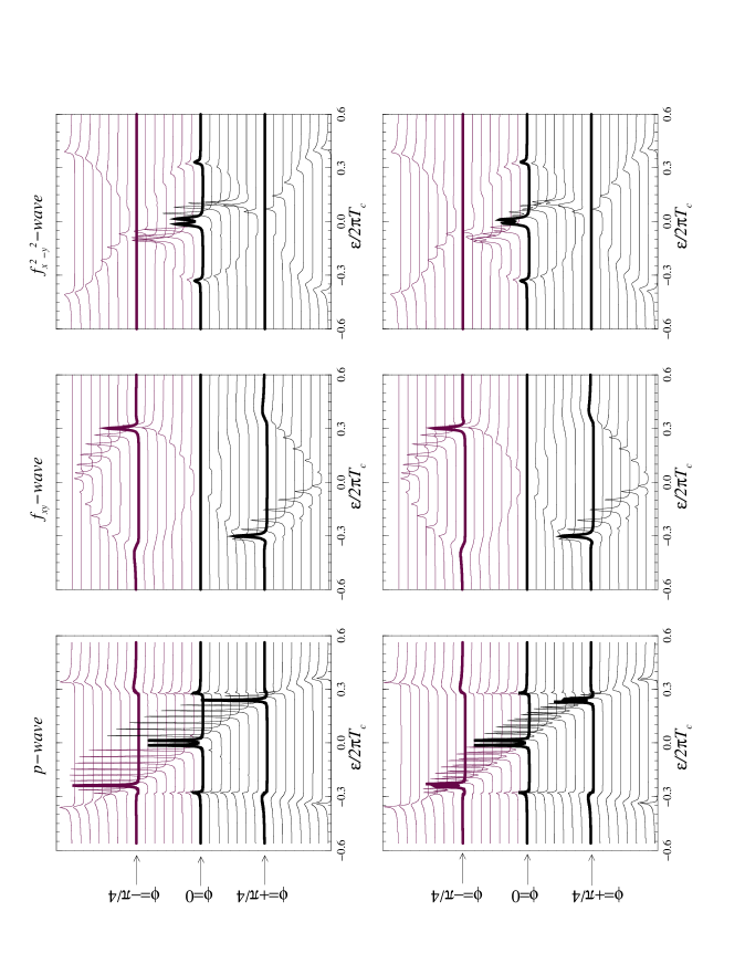
FIG. 3.: The local angular resolved surface density of states shown (left to right) for the $p$-wave, the $f_{xy}$-wave and the $f_{x^{2}-y^{2}}$-wave junctions. The transparency ${\cal D}=0.01$ and the phase difference is zero. The top row are all symmetric junctions ($\tilde{\chi}=+1$) while the bottom row are junctions with opposite chiralities ($\tilde{\chi}=-1$). The DOS is given in the interval $\varphi=-\pi/2$ to $\varphi=\pi/2$ in equally spaced steps.

  

In figure 3 we show the numerically computed local interface DOS, using the self-consistently determined self-energies. The angle-resolved DOS in the left superconductor is defined as

$$N(\varphi,\varepsilon)=-\frac{1}{2}N_{f}\mbox{Im}\bigg{\{}\mbox{Tr}[\hat{\tau}_{3}\hat{g}(\varphi,0_{-};\varepsilon)]\bigg{\}}$$ (15)

and calculated at zero phase difference with one and the same transparency ${\cal D}=0.01$ for all momentum directions. Here and below we use the normalization condition $\hat{g}^{2}=-1$ for the quasiclassical Green’s function. The DOS in the right superconductor are for these symmetric junctions simply related to the DOS in the left by substituting $\varepsilon^{r}=-\tilde{\chi}\cdot\varepsilon^{l}$. Qualitatively, peak positions are well described by Eqs.(6) and (7), obtained in the tunneling limit. The fine structure of the peaks are due to a finite transmission. The density of states for junctions with bound states dispersing in $\mathchoice{{\hbox{\boldmath$\displaystyle p$}}}{{\hbox{\boldmath$\textstyle p$}}}{{\hbox{\boldmath$\scriptstyle p$}}}{{\hbox{\boldmath$\scriptscriptstyle p$}}}_{f}$ and having $\varepsilon_{B}=0$ at $\varphi=0$, i.e. for the $p$-wave and for the $f_{x^{2}-y^{2}}$-wave pairings, show a split DOS, by an amount $\sqrt{\cal D}$ at $\varepsilon=0$ (in accordance with Eqs.(3) and (8); see also (13) and (14)). At finite angles $\varphi$ the DOS show the predicted dependence on the relative chirality of the two superconductors. For the $\tilde{\chi}=+1$ junction, since $\varepsilon^{r}_{B,{\cal D}=0}=-\varepsilon^{l}_{B,{\cal D}=0}$, there is only a very small spectral weight in the DOS from the bound state $\varepsilon^{r}_{B,{\cal D}}$ induced in the left superconductor through the junction in the tunneling limit. For the $\tilde{\chi}=-1$ junction we have $\varepsilon^{r}_{B,{\cal D}=0}=\varepsilon^{l}_{B,{\cal D}=0}$. Hence, there is almost equal weight in the two states split around $\varepsilon_{B,{\cal D}=0}(\varphi)$. The split again $\propto\sqrt{{\cal D}}$ (see Eq.(14)). For small angles $(\varphi\approx 0)$ the $p$-wave and the $f_{x^{2}-y^{2}}$-wave superconductors lead to qualitatively similar DOS. For the $f_{xy}$-wave superconductors the chiral branches take on low energies only for momentum directions close to the nodes of the order parameter and the main part of the low-energy spectral weight belongs to glancing trajectories. The $f_{xy}$-wave with $\tilde{\chi}=-1$ does not show splitting if $\Phi=0$, in accordance with Eq.(10).

III Low temperature anomaly of the Josephson current

A The Josephson current in quantum point contacts

Consider the Josephson current across junctions with chiral interface states first assuming spatially constant order parameters. For a quantum point contact we can find the current in symmetric junctions (with $\tilde{\chi}=1$) as[70, 71, 72, 73] $j=2e\sum\limits_{a}\frac{\displaystyle d\varepsilon_{B}^{a}}{\displaystyle d\Phi}n_{f}(\varepsilon_{B}^{a})=-2e\sum\limits_{\varepsilon_{B}^{a}>0}\frac{\displaystyle d\varepsilon_{B}^{a}}{\displaystyle d\Phi}\tanh\frac{\displaystyle\varepsilon_{B}^{a}}{\displaystyle 2T}$. Here the spectrum is presumably even and the sum is taken over different channels. Making use of the relationship $\frac{\displaystyle d\varepsilon_{B}}{\displaystyle d\Phi}=\frac{\displaystyle-|\Delta|^{2}{\cal D}\sin\Phi}{\displaystyle 4\varepsilon_{B}}$, which easily follows from Eqs.(3)-(5) for all pairings we discuss, leads to the Josephson current

$$j=\frac{\displaystyle e|\Delta|^{2}{\cal D}\sin\Phi}{\displaystyle 2\varepsilon_{B}}\tanh\frac{\displaystyle\varepsilon_{B}}{\displaystyle 2T}$$ (16)

for one channel in a quantum point contact.

Eq.(16) is applicable also to contacts between isotropic s-wave superconductors. In this case, however, the bound state energies are mainly on the order of $\Delta$. They can take low-energy values only in highly transparent junctions and for phase differences $\Phi$ in a narrow vicinity of $\pi$. There are well-known specific features of the Josephson current manifested in conventional superconductors with micro-constrictions[76]. For the phase difference $\Phi\approx\pi$, however, $\sin\Phi$ in Eq.(16) is very small as well, precluding the low-temperature features of the Josephson critical current we discuss below. By contrast, under certain conditions chiral bound states can take low energy values at any phase difference $\Phi$. For the $p$-wave and the $f_{x^{2}-y^{2}}$-wave order parameters, as well as for the three-dimensional $E_{1g}$-type of pairing, this is the case, in particular, in tunnel junctions (${\cal D}\ll 1$) for quasiparticles with momenta aligned almost (or exactly) parallel to the interface normal $\varphi\approx 0,\pi$.

For a nonzero energy and sufficiently low temperatures, when $T\ll\varepsilon_{B}$, we get from Eq.(16) the zero-temperature value of the Josephson current $j=\frac{\displaystyle e|\Delta_{0}|^{2}{\cal D}\sin\Phi}{\displaystyle 2\varepsilon_{B}}$. Here $\Delta_{0}$ is the zero-temperature order parameter. Hence, the zero-temperature critical current is much greater for channels with $\varepsilon_{B}\ll|\Delta_{0}|$, as compared with channels, where $\varepsilon_{B}\sim|\Delta_{0}|$, for given $\Phi$, ${\cal D}$ and $|\Delta_{0}|$.

If $\varepsilon_{B}\ll T\ll T_{c}$, which can be satisfied only by low-energy states, we find from Eq.(16) that the Josephson current can vary substantially in the low-temperature region being inversely proportional to the temperature: $j=\frac{\displaystyle e|\Delta_{0}|^{2}{\cal D}\sin\Phi}{\displaystyle 4T}$.

To be specific, consider the $p$-wave order parameter and $\varepsilon_{B}=\Delta_{b}^{p}\sqrt{\displaystyle{\cal R}\sin^{2}\varphi+{\cal D}\cos^{2}\frac{\displaystyle\Phi}{\displaystyle 2}}$. Here $\varphi$ is the parameter characterizing the quantum state in the channel. The bound state energy is small, i.e. $\varepsilon_{B}\ll\Delta_{b}^{p}$, for example if $|\varphi|\ll 1$ and ${\cal D}\ll 1$. Then the zero-temperature current is quite large and equal to either $\frac{\displaystyle e\Delta_{b,0}^{p}{\cal D}\sin\Phi}{\displaystyle 2|\varphi|}$ when ${\rm max}\left(\frac{\displaystyle T}{\displaystyle\Delta_{b}^{p}},\sqrt{\displaystyle{\cal D}}\left|\cos\frac{\displaystyle\Phi}{\displaystyle 2}\right|\right)\ll|\varphi|\ll 1$ or to $e\Delta_{b,0}^{p}\sqrt{{\cal D}}{\rm sgn}\left(\cos\frac{\displaystyle\Phi}{\displaystyle 2}\right)\sin\frac{\displaystyle\Phi}{\displaystyle 2}$ if $\frac{\displaystyle T}{\displaystyle\Delta_{b}^{p}}\ll|\varphi|\ll\sqrt{\displaystyle{\cal D}}\left|\cos\frac{\displaystyle\Phi}{\displaystyle 2}\right|\ll 1$. In the last case the Josephson current in the tunnel junction turns out to be proportional to $\sqrt{\cal D}$, in contrast to the linear dependence on ${\cal D}$ of the conventional tunneling current. As we see, the low-temperature value of the Josephson current depends on the dimensionless parameter $\sqrt{{\cal D}}|\Delta||\cos(\Phi/2)|/T$ containing the transparency. This parameter appears from the expression for the energy of the interface bound states when comparing it with the temperature. At sufficiently low temperatures the parameter is large even if ${\cal D}\ll 1$.

It follows from Eqs.(3)-(5) that the condition $\varepsilon_{B}(\mathchoice{{\hbox{\boldmath$\displaystyle p$}}}{{\hbox{\boldmath$\textstyle p$}}}{{\hbox{\boldmath$\scriptstyle p$}}}{{\hbox{\boldmath$\scriptscriptstyle p$}}}_{f})\ll\Delta(\mathchoice{{\hbox{\boldmath$\displaystyle p$}}}{{\hbox{\boldmath$\textstyle p$}}}{{\hbox{\boldmath$\scriptstyle p$}}}{{\hbox{\boldmath$\scriptscriptstyle p$}}}_{f})$ is satisfied for any phase difference for the tunnel junctions with $\varphi$ near the nodes at $\varphi_{0}\approx 0,\pi$ of the chiral bound states for the $p$-wave, the $f_{x^{2}-y^{2}}$-wave and the three-dimensional $E_{1g}$ order parameters. For the $f_{xy}$-wave order parameter the above condition takes place only for glancing trajectories, which contribute negligibly to the Josephson current. For the three-dimensional $E_{2u}$ type of pairing the nodes of the bound states, not coinciding with the nodes of the order parameter, lie at $\varphi^{t}_{0}=\pm\pi/4,\pm 3\pi/4$. For this reason the $E_{2u}$ pairing (UPt₃) has a contribution from the low-energy chiral surface bound states to the Josephson current that turns out to be especially sensitive to the momentum dependence of the tunneling probability, ${\cal D}(\mathchoice{{\hbox{\boldmath$\displaystyle p$}}}{{\hbox{\boldmath$\textstyle p$}}}{{\hbox{\boldmath$\scriptstyle p$}}}{{\hbox{\boldmath$\scriptscriptstyle p$}}}_{f})$. This contrasts the $E_{1g}$ pairing as well as the $p$- and $f$-wave superconductors. The sensitivity is associated with the fact that the transparency of a barrier quickly diminishes with increasing a deviation of the momentum direction from the surface normal (unless the barrier is sufficiently thin). Thus, the transmission can become quite small for momenta with $\varphi^{t}_{0}=\pm\pi/4$ or $\pm 3\pi/4$. For example, a model for the tunneling barrier with a uniform probability distribution within an acceptance cone about the interface normal, and zero outside the cone, the effect considered is entirely absent unless the acceptance cone contains (or its boundary is very close to) $\varphi^{t}_{0}=\pm\pi/4,\pm 3\pi/4$. For a narrow Gaussian-distribution model the tunneling at $\varphi^{t}_{0}=\pm\pi/4,\pm 3\pi/4$ is not strictly zero, although exponentially small. For a sufficiently thin and high barrier, however, the transparency is approximately proportional to $(\mathchoice{{\hbox{\boldmath$\displaystyle n$}}}{{\hbox{\boldmath$\textstyle n$}}}{{\hbox{\boldmath$\scriptstyle n$}}}{{\hbox{\boldmath$\scriptscriptstyle n$}}}\cdot\mathchoice{{\hbox{\boldmath$\displaystyle p$}}}{{\hbox{\boldmath$\textstyle p$}}}{{\hbox{\boldmath$\scriptstyle p$}}}{{\hbox{\boldmath$\scriptscriptstyle p$}}}_{f})^{2}$ and then the contribution to the Josephson current from the low-energy chiral surface states becomes important even for the $E_{2u}$-triplet pairing. In the last case the particular $\mathchoice{{\hbox{\boldmath$\displaystyle p$}}}{{\hbox{\boldmath$\textstyle p$}}}{{\hbox{\boldmath$\scriptstyle p$}}}{{\hbox{\boldmath$\scriptscriptstyle p$}}}_{f}$-dependence of the tunneling probability is ${\cal D}(\mathchoice{{\hbox{\boldmath$\displaystyle p$}}}{{\hbox{\boldmath$\textstyle p$}}}{{\hbox{\boldmath$\scriptstyle p$}}}{{\hbox{\boldmath$\scriptscriptstyle p$}}}_{f})={\cal D}_{0}\cos^{2}\varphi$ for two-dimensional models with a cylindrical Fermi surface and ${\cal D}(\mathchoice{{\hbox{\boldmath$\displaystyle p$}}}{{\hbox{\boldmath$\textstyle p$}}}{{\hbox{\boldmath$\scriptstyle p$}}}{{\hbox{\boldmath$\scriptscriptstyle p$}}}_{f})={\cal D}_{0}\sin^{2}\theta\cos^{2}\varphi$ for three-dimensional models with a spherical Fermi surface.

B The critical current in classical tunnel junctions

The low-temperature anomalous behavior of the Josephson current described above is quite similar to what was theoretically found for the case of $d$-wave superconductors in the presence of zero- and low-energy surface and interface states[20, 21, 22]. However, the similarity takes place only in considering one channel, which is appropriate to quantum point contacts. In classical junctions, where quasiparticles have various momentum directions, the parameter $\varphi$ appears in the expression for the Josephson current as an integration variable in averaging over the Fermi surface. If the bound states are substantially dispersive, manifesting strong dependence of their energy on the momentum direction, the averaging can noticeably weaken the low-temperature deviations of the Josephson current from its conventional behavior.

The eventual result can be easily understood qualitatively, if one notices that the integration of the $1/|\varphi|$-term (see the preceding subsection) over the interval $\left({\rm max}\left(\frac{\displaystyle T}{\displaystyle\Delta_{b}^{p}},\sqrt{\displaystyle{\cal D}}\left|\cos\frac{\displaystyle\Phi}{\displaystyle 2}\right|\right),\varphi_{c}\right)$ (where $\varphi_{c}\ll 1$) leads to logarithmic low-temperature dependences on the temperature or the transparency. Below we present a more careful analysis of the low-temperature features of the critical current.

For a classical symmetric junction (with $\tilde{\chi}=1$) between quasi-two-dimensional superconductors we get instead of Eq.(16):

$$j_{x}=\int\limits_{-\frac{\pi}{2}}^{+\frac{\pi}{2}}d\varphi\frac{\displaystyle e{\rm v}_{f}N_{f}{\cal D}(\varphi)\cos\varphi\sin{\Phi}|\Delta(\varphi)|^{2}}{\displaystyle 2\varepsilon_{B}(\varphi)}\tanh\left(\frac{\displaystyle\varepsilon_{B}(\varphi)}{\displaystyle 2T}\right).$$ (17)

Assuming the logarithmic functions mentioned above to be large, one can use a logarithmic approximation, considering only a part of the integral in Eq.(17), which contains the zero-level crossing of the chiral branches $\mathchoice{{\hbox{\boldmath$\displaystyle p$}}}{{\hbox{\boldmath$\textstyle p$}}}{{\hbox{\boldmath$\scriptstyle p$}}}{{\hbox{\boldmath$\scriptscriptstyle p$}}}_{f,0}$. Then for a symmetric tunnel junction between quasi-two-dimensional superconductors with cylindrical Fermi surfaces we get from Eq.(17)

  

$$j_{x}\approx\!\!\!\sum_{\stackrel{{\scriptstyle\varphi_{0}}}{{\mathchoice{{\hbox{\boldmath$\displaystyle p$}}}{{\hbox{\boldmath$\textstyle p$}}}{{\hbox{\boldmath$\scriptstyle p$}}}{{\hbox{\boldmath$\scriptscriptstyle p$}}}_{f,x}>0}}}e{\rm v}_{f}N_{f}{\cal D}(\varphi_{0})\cos\varphi_{0}\sin{\Phi}|\Delta(\varphi_{0})|^{2}\int\limits_{\varphi_{0}}^{\varphi_{0}+\delta\varphi_{c}}d\varphi\frac{\displaystyle 1}{\displaystyle\varepsilon_{B}(\varphi)}\tanh\left(\frac{\displaystyle\varepsilon_{B}(\varphi)}{\displaystyle 2T}\right),$$ (18)

where $\varepsilon_{B}(\varphi)$ is defined by Eqs.(3) and (4), $\varepsilon_{B}(\varphi)\Big{|}_{{\cal D}=0}$ is to be evaluated to linear order in $\delta\varphi$. $\delta\varphi_{c}$ is a cut-off parameter. The sum is taken over those $\varphi_{0}$, which correspond to $\mathchoice{{\hbox{\boldmath$\displaystyle p$}}}{{\hbox{\boldmath$\textstyle p$}}}{{\hbox{\boldmath$\scriptstyle p$}}}{{\hbox{\boldmath$\scriptscriptstyle p$}}}_{f,x}>0$. For the $p$- or the $f_{x^{2}-y^{2}}$-wave pairing only $\varphi^{p,f}_{0}=0$ satisfies the condition. In the case of three-dimensional superconductors with the $E_{2u}$- or the $E_{1g}$-pairings, an additional integration $\int\limits_{0}^{\pi/2}\sin^{2}\theta d\theta$ has to be carried out in Eq.(17), where ${\cal D}$, $|\Delta|$ and $\varepsilon_{B}$, depend on both $\varphi$ and $\theta$. For the $E_{2u}$ and the $E_{1g}$ one should consider variations $\delta\varphi$ from $\varphi^{t}_{0}=\pm\pi/4$ and $\varphi^{s}_{0}=0$ respectively.

The contribution to the Josephson current from low-energy bound states in the tunnel junctions can be also calculated analytically taking into account the surface pair-breaking. Indeed, from Eqs.(13), (40) we easily get $\frac{\displaystyle d\varepsilon_{B}}{\displaystyle d\Phi}=\frac{\displaystyle-|\tilde{\Delta}|^{2}{\cal D}\sin\Phi}{\displaystyle 4\varepsilon_{B}}$, where the effective order parameter $|\tilde{\Delta}(\mathchoice{{\hbox{\boldmath$\displaystyle p$}}}{{\hbox{\boldmath$\textstyle p$}}}{{\hbox{\boldmath$\scriptstyle p$}}}{{\hbox{\boldmath$\scriptscriptstyle p$}}}_{f},0)|$ near the nodes of the bound states is defined in the right half space

$$\frac{\displaystyle 1}{\displaystyle|\tilde{\Delta}(\mathchoice{{\hbox{\boldmath$\displaystyle p$}}}{{\hbox{\boldmath$\textstyle p$}}}{{\hbox{\boldmath$\scriptstyle p$}}}{{\hbox{\boldmath$\scriptscriptstyle p$}}}_{f},0)|}=\frac{\displaystyle 2}{\displaystyle|{\rm v}_{f,x}(\mathchoice{{\hbox{\boldmath$\displaystyle p$}}}{{\hbox{\boldmath$\textstyle p$}}}{{\hbox{\boldmath$\scriptstyle p$}}}{{\hbox{\boldmath$\scriptscriptstyle p$}}}_{f})|}\int\limits_{0}^{\infty}e^{-\frac{2}{{\rm v}_{f,x}(\mathchoice{{\hbox{\boldmath$\displaystyle p$}}}{{\hbox{\boldmath$\textstyle p$}}}{{\hbox{\boldmath$\scriptstyle p$}}}{{\hbox{\boldmath$\scriptscriptstyle p$}}}_{f})}\int\limits_{0}^{x_{1}}|\Delta(\mathchoice{{\hbox{\boldmath$\displaystyle p$}}}{{\hbox{\boldmath$\textstyle p$}}}{{\hbox{\boldmath$\scriptstyle p$}}}{{\hbox{\boldmath$\scriptscriptstyle p$}}}_{f},x_{2})|\sin\left(\eta(\mathchoice{{\hbox{\boldmath$\displaystyle p$}}}{{\hbox{\boldmath$\textstyle p$}}}{{\hbox{\boldmath$\scriptstyle p$}}}{{\hbox{\boldmath$\scriptscriptstyle p$}}}_{f},x_{2})-\phi(\mathchoice{{\hbox{\boldmath$\displaystyle p$}}}{{\hbox{\boldmath$\textstyle p$}}}{{\hbox{\boldmath$\scriptstyle p$}}}{{\hbox{\boldmath$\scriptscriptstyle p$}}}_{f},x_{2})\right)dx_{2}}dx_{1}\enspace\enspace,$$ (19)

  

and analogously in the left half space. Hence, spatial dependence of the order parameters introduces in this case the only modification in Eq.(18): the order parameter $|\Delta(\varphi)|$ should be replaced there by the effective surface order parameter $|\tilde{\Delta}(\varphi)|$.

For temperatures $\sqrt{{\cal D}(\mathchoice{{\hbox{\boldmath$\displaystyle p$}}}{{\hbox{\boldmath$\textstyle p$}}}{{\hbox{\boldmath$\scriptstyle p$}}}{{\hbox{\boldmath$\scriptscriptstyle p$}}}_{f,0})}|\tilde{\Delta}(\mathchoice{{\hbox{\boldmath$\displaystyle p$}}}{{\hbox{\boldmath$\textstyle p$}}}{{\hbox{\boldmath$\scriptstyle p$}}}{{\hbox{\boldmath$\scriptscriptstyle p$}}}_{f,0})||\cos(\Phi/2)|\ll T\ll\Delta_{b}\delta\varphi_{c}<T_{c}$ one can put $\tanh\left(\varepsilon_{B}(\varphi)/2T\right)\approx 1$ near the upper limit of the integral in Eq.(18) and use Eqs.(3) and (4) for $\varepsilon^{p,f_{x^{2}-y^{2}}}_{B}(\varphi),\varepsilon^{s,t}_{B}(\theta,\varphi)\propto\delta\varphi$. Then we find a logarithmic temperature dependence of the integral near the lower limit $\varphi_{0}$ in Eq.(18). Qualitatively, the temperature is a lower cut of the integral, but for fixing numerical factors we checked its asymptotic behavior numerically. Thus, at sufficiently low temperatures, when contributions to the current from quasiparticles with energies the order of $|\Delta(\mathchoice{{\hbox{\boldmath$\displaystyle p$}}}{{\hbox{\boldmath$\textstyle p$}}}{{\hbox{\boldmath$\scriptstyle p$}}}{{\hbox{\boldmath$\scriptscriptstyle p$}}}_{f})|$ already take their zero-temperature value, the Josephson current associated with the low-energy part of the chiral bound states and described by Eq.(18) can still grow logarithmically with the decreasing temperature. As a result, the total Josephson current can be represented for the low-temperature interval $\sqrt{{\cal D}(\mathchoice{{\hbox{\boldmath$\displaystyle p$}}}{{\hbox{\boldmath$\textstyle p$}}}{{\hbox{\boldmath$\scriptstyle p$}}}{{\hbox{\boldmath$\scriptscriptstyle p$}}}_{f,0})}|\tilde{\Delta}(\mathchoice{{\hbox{\boldmath$\displaystyle p$}}}{{\hbox{\boldmath$\textstyle p$}}}{{\hbox{\boldmath$\scriptstyle p$}}}{{\hbox{\boldmath$\scriptscriptstyle p$}}}_{f,0})||\cos(\Phi/2)|\ll T\ll T_{c}$ as

$$j_{x}(T)=aj_{c,0}\ln\left(\frac{\displaystyle b\Delta_{b}}{\displaystyle T}\right)\sin\Phi\enspace,$$ (20)

where $j_{c,0}=LeN_{f}{\rm v}_{f}{\cal D}_{0}\Delta_{b}$ ($L^{p}=2/3$, $L^{f_{x^{2}-y^{2}}}\approx 0.45$, $L^{f_{xy}}=2/5$, $L^{s}=1/9$, $L^{t}=2/21$), $\Delta_{b}=\Delta^{p,f_{x^{2}-y^{2}},f_{xy},s,t}_{b}$, $a$ and $b$ are constants the order of unity. In our analytical results here and below the transparency is taken for high and thin potential barriers as it was represented in the end of the preceding subsection. Further, disregarding surface pair-breaking, we calculate analytically a total Josephson current and find at low temperatures after the comparison with Eq.(20) $a^{p}=3/2$, $b^{p}\approx 0.69$, $a^{f_{x^{2}-y^{2}}}\approx 2.23$, $b^{f_{x^{2}-y^{2}}}\approx 0.44$, $a^{s}=3/2$, $b^{s}\approx 0.23$, $a^{t}=3/4\sqrt{2}$, $b^{t}\approx 0.95$. In neglecting not only a surface pair-breaking (that is a spatial dependence of the order parameter), but the presence of any surface bound states at all, one can use spatially constant (bulk) values of Green’s functions for the calculation of the Josephson current. This oversimplified approach leads for the symmetric tunnel junction to the Josephson critical current $j_{c,0}$. As the argument of the logarithmic function in Eq.(20) is supposed to be quite large (for the logarithmic approximation to be valid), the Josephson current $j_{x}(T)$ can noticeably exceed $j_{c,0}$.

For temperatures $T\ll\sqrt{{\cal D}_{0}}\Delta_{b}|\cos(\Phi/2)|$ the lower cut of the integral is associated with the transparency of the barrier and we find from Eq.(18)

$$j_{x}(0)=aj_{c,0}\ln\left(\frac{\displaystyle d}{\displaystyle\sqrt{{\cal D}_{0}}|\cos(\Phi/2)|}\right)\sin\Phi\enspace.$$ (21)

The logarithmic function in Eq.(21) is supposed to take large values as well. Disregarding surface pair breaking, we find $d^{p}\approx 1.21$, $d^{f_{x^{2}-y^{2}}}\approx 0.78$, $d^{s}\approx 1.21$, $d^{t}\approx 1.88$.

Based on Eqs.(8)-(10), one can easily get the Josephson current in junctions with opposite chiralities. We do not present here the corresponding analytical results in detail, since there is no unconventional low-temperature increase in the critical current in the case $\tilde{\chi}=-1$. In disregarding surface pair breaking the Josephson current in tunnel junction at $T\ll T_{c}$ in the case $\tilde{\chi}=-1$ is written as

$$j_{x}=uj_{c,0}\sin\Phi\enspace,$$ (22)

where $u^{p}=9/8$,  $u^{f_{xy}}=5/3$,  $u^{f_{x^{2}-y^{2}}}\approx 1.95$,  $u^{s}=9/8$,  $u^{t}\approx 0.142$. The “reference” current $j_{c,0}$ is taken here the same as in Eqs.(20) and (21) in order to make clear that the Josephson current in the case of opposite chiralities is of the conventional order of magnitude without any logarithmic enhancement. The smaller numerical factor $u^{t}$ is associated with the lower transparency for $\varphi^{t}_{0}=\pm\pi/4$ as compared with $\varphi^{p,f_{x^{2}-y^{2}},s}_{0}=0$. Surface chiral bound states in the whole range of subgap energies form the current in the particular case, even at low temperatures. One can show that the low-energy chiral quasiparticle states lead to a current which is reduced compared to Eq.(22) by the small cut-off parameter $\delta\varphi_{c}$ and it does not matter whether the surface pair breaking is taken into account or not.

Another reason for choosing the “reference” current $j_{c,0}$ in the case $\tilde{\chi}=-1$ same as for $\tilde{\chi}=1$, is that in neglecting both the surface pair breaking and the presence of Andreev surface bound states, and simply using the bulk expressions for the Green’s functions, the tunnel Josephson critical current across the domain wall ($\tilde{\chi}=-1$) vanishes. This in sharp contrast with Eq.(22). For a vanishing Josephson current one needs, for example, different projections of the orbital angular momentum, i.e. different values of $l_{z}$, of the Cooper pairs in the left and the right superconductors together with a conservation of $l_{z}$ in the tunneling process. The current vanishes, for instance, if $l_{z}$ is along the interface normal and the interface is symmetric with respect to the rotations around the normal[38, 39]. As we demonstrate in Eq.(22), if $l_{z}$ is along an axis parallel to the interface, the interface influence results in interface bound states and the possibility of a nonzero tunneling of Cooper pairs. Eq.(22) applies to tunnel junctions. Effects of high transparency can also lead to finite critical current[77].

On account of the bound states, the Green’s function depends on the distance from the surface even when disregarding a spatial dependence of the order parameter. There is an important qualitative difference between the surface and the bulk values of the propagators as a function of momentum direction. In particular, the angle $\varphi$ is an important part of the phase not only for the chiral order parameter, but for the bulk value of the off-diagonal components of the Green’s function as well. Since we consider the $z$-axis to be parallel to the surface, the surface breaks the conservation of the projection of the angular momentum. For this reason the angle $\varphi$ drops out from the phase in the surface value of the off-diagonal components. This can be obtained on account of the continuity of the quasiclassical Green’s function, taken for incoming and outgoing trajectories (with the angles $\varphi$ and $\pi-\varphi$ respectively) at the impenetrable surface. Thus, on account of the surface effects, the Josephson tunnel current across the domain wall is of the conventional value (see Eq.(22)).

The logarithmic behavior of the critical current found above for classical symmetric junctions with $\tilde{\chi}=1$, is observable only at sufficiently low temperatures and at low junction transparencies when the logarithmic approximation can be justified. This is demonstrated in Figure 4, where we show the result of numerical calculations for the temperature dependence of the critical current for different values of barrier transparency.

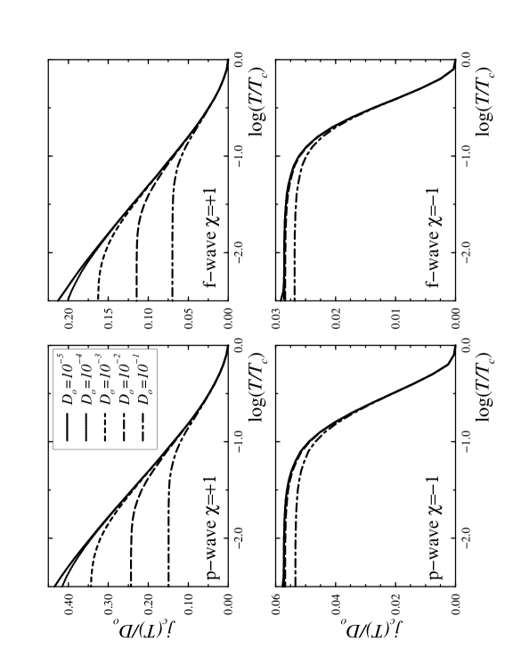
FIG. 4.: The temperature dependence of the critical current divided by the maximal transparency ${\cal D}_{0}$ plotted for different values of ${\cal D}_{0}$. The junctions are modelled with the angle dependent transparency ${\cal D}(\varphi)={\cal D}_{0}\exp(-16\sin^{2}\varphi)$. To the left we show two coupled p-wave superconductors and to the right two $f_{x^{2}-y^{2}}$-wave ones.

As seen for the ${\tilde{\chi}}=+1$ junctions, the term ${\cal D}_{0}\ln{\cal D}_{0}$ is present in the tunneling limit in the dependence of the zero-temperature critical current on the transparency (see Eq.(21)). Further, the low-temperature range, where the critical current linearly depends on $\ln T$ (see Eq.(20)), becomes well pronounced only for transparencies less than $10^{-2}$. The finite transparency efficiently cuts off the logarithmic temperature dependence of the critical current. The lower the transparency, the larger the low-temperature range. The characteristic temperature, below which the transparency influence becomes noticeable, is proportional to $\sqrt{{\cal D}}$, again in agreement with our analytical results.

In Fig. 5 we show the analogous result for the $f_{xy}$-wave superconductor. Since the low-energy contribution from the bound states is associated in this case only with glancing trajectories, there are no anomalies in the critical current.

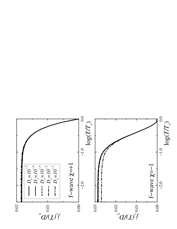
FIG. 5.: The temperature dependence of the critical current calculated as in Fig. 4 but for the $f_{xy}$-wave superconductor.

C Effects of broadening of the bound states

Broadening of the chiral low-energy bound states can substantially modify the low-temperature behavior of the critical current found above. Even a small broadening $\gamma\ll\Delta_{b}$ have a profound influence on the low-energy parts of chiral branches. We take a small broadening into account in the pole-like term of the retarded quasiclassical Green’s function, where we simply replace the factor $1/[\varepsilon-\varepsilon_{B}(\mathchoice{{\hbox{\boldmath$\displaystyle p$}}}{{\hbox{\boldmath$\textstyle p$}}}{{\hbox{\boldmath$\scriptstyle p$}}}{{\hbox{\boldmath$\scriptscriptstyle p$}}}_{f})]$ with $1/[\varepsilon-\varepsilon_{B}(\mathchoice{{\hbox{\boldmath$\displaystyle p$}}}{{\hbox{\boldmath$\textstyle p$}}}{{\hbox{\boldmath$\scriptstyle p$}}}{{\hbox{\boldmath$\scriptscriptstyle p$}}}_{f})+i\gamma]$, analogously to what is done in[26]. This slightly modifies the analysis of Ref. [21] for the contribution from the low-energy bound states to the Josephson current in tunnel junctions. We evaluate the current in the tunneling limit assuming the momentum independent broadening substantially greater than the low-energy bound state and the temperature: $T,\sqrt{{\cal D}_{0}}\Delta_{b}|\cos(\Phi/2)|\ll\gamma\ll\Delta_{b}$. The lower cut of the integral in Eq.(18) is associated in this case with $\gamma$ rather than the temperature or the bound state energy. Then we find for the Josephson current

$$j_{x}(0)=aj_{c,0}\ln\left(\frac{\displaystyle w\Delta_{b}}{\displaystyle\gamma}\right)\sin\Phi\enspace.$$ (23)

For spatially constant order parameters we get $w^{p}\approx 0.61$, $w^{f_{x^{2}-y^{2}}}\approx 0.39$, $w^{s}\approx 0.21$, $w^{t}\approx 0.84$.

There are various contributions to the broadening of the bound states. These are in particular associated with surface roughness, non-magnetic and magnetic impurities, and with inelastic scattering. We assume here that non-magnetic impurities dominate the scattering and thus the broadening. Then we calculate the effect of small scattering rates on the behavior of the Josephson current at low temperatures using the usual t-matrix approximation and assuming an isotropic impurity potential, $u$. The impurity self energy is in this case

$$\hat{\Sigma}(\varepsilon)=\Gamma{\langle\hat{g}(\varepsilon)\rangle\over{1-\sigma(1+\langle\hat{g}(\varepsilon)\rangle^{2}})}\enspace.$$ (24)

where the scattering strength $\sigma=\sin^{2}\delta_{s}$ ($\delta_{s}$ is the s-wave scattering phase-shift, $0\leq\delta_{s}\leq\frac{\pi}{2}$) and the scattering rate, $\Gamma$, parameterize $u$ and the impurity density $n_{imp}$ as

$$\sigma=\frac{(\pi N_{f}u)^{2}}{1+(\pi N_{f}u)^{2}}\qquad{\Gamma}=\frac{\pi N_{f}u^{2}}{1+(\pi N_{f}u)^{2}}\,n_{imp}\enspace.$$ (25)

Due to the low-energy bound states, the Matsubara Green’s function can take quite large values in the low-temperature region, if the broadening and the transparency are sufficiently small. However, the low-energy states form only a small part of the chiral branches, i.e. for most of the quasiparticle trajectories the energy of the chiral states is the order of $\Delta_{b}(\mathchoice{{\hbox{\boldmath$\displaystyle p$}}}{{\hbox{\boldmath$\textstyle p$}}}{{\hbox{\boldmath$\scriptstyle p$}}}{{\hbox{\boldmath$\scriptscriptstyle p$}}}_{f})$. For this reason the quasiclassical propagator for the chiral superconductor, averaged over the Fermi surface, $\langle g(\varepsilon)\rangle$, does not take large values but is of the order of unity or less. This differs greatly from the case of a 45^∘-oriented d-wave superconductor for which each trajectory has an Andreev bound state at zero energy. There $\langle g(\varepsilon)\rangle$ can take large values along with the pole-like term in the quasiclassical Green’s function[28].

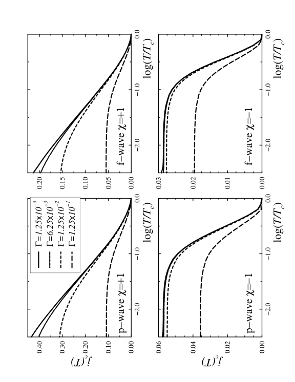
FIG. 6.: The temperature dependence of the critical current for a junction modelled with the transparency ${\cal D}(\varphi)={\cal D}_{0}\exp(-16\sin^{2}\varphi)$ and ${\cal D}_{0}=10^{-5}$. $j_{c}(T)$ is calculated at different scattering rates $\Gamma/T_{c}$. The scattering strength is weak and put to $\sigma=0.1$.

In Fig. 6 we show the influence of impurity effects on the temperature dependence of critical current. In order to get a wide range of well pronounced dependence of the critical current on the small broadening, we take the extreme tunnel limit and put ${\cal D}_{0}=10^{-5}$. One can see from the Fig. 6, that for observing the logarithmic low-temperature enhancement of $j_{c}$, one needs superconductors of high purity.

IV Summary

Chiral interface Andreev bound states have been obtained and studied above both analytically and numerically. We showed, that the low-energy chiral states results in the low-temperature enhancement of the Josephson current between clean chiral superconductors in symmetric tunnel junctions. The enhancement is more pronounced in quantum point contacts. In classical junctions the zero-temperature current acquires an additional logarithmic dependence on low transparency or on the broadening of the bound states. Under the conditions considered, the Josephson current through the domain wall does not vanish due to the bound state contribution.

V Acknowledgments

Yu.B. would like to thank T. Kopp and J. Mannhart for kind hospitality during his stay in University of Augsburg, where a part of this work was carried out. This work was supported in part by BMBF 13N6918/1 (Yu.B.), by the Russian Foundation for Basic Research under Grant No. 99-02-17906 (Yu.B. and A.B.) and by the Swedish Natural Science Research Council (M.F.).

Energies of the interface bound states

In the presence of a quasiparticle bound state $\varepsilon_{B}(\mathchoice{{\hbox{\boldmath$\displaystyle p$}}}{{\hbox{\boldmath$\textstyle p$}}}{{\hbox{\boldmath$\scriptstyle p$}}}{{\hbox{\boldmath$\scriptscriptstyle p$}}}_{f})$ the quasiclassical retarded propagator $\hat{g}$ has a pole at $\varepsilon=\varepsilon_{B}(\mathchoice{{\hbox{\boldmath$\displaystyle p$}}}{{\hbox{\boldmath$\textstyle p$}}}{{\hbox{\boldmath$\scriptstyle p$}}}{{\hbox{\boldmath$\scriptscriptstyle p$}}}_{f})$. One can introduce the residue of the propagator $\hat{g}$ as

$$\hat{\tilde{g}}(\mathchoice{{\hbox{\boldmath$\displaystyle p$}}}{{\hbox{\boldmath$\textstyle p$}}}{{\hbox{\boldmath$\scriptstyle p$}}}{{\hbox{\boldmath$\scriptscriptstyle p$}}}_{f},\mathchoice{{\hbox{\boldmath$\displaystyle r$}}}{{\hbox{\boldmath$\textstyle r$}}}{{\hbox{\boldmath$\scriptstyle r$}}}{{\hbox{\boldmath$\scriptscriptstyle r$}}};\varepsilon_{B}(\mathchoice{{\hbox{\boldmath$\displaystyle p$}}}{{\hbox{\boldmath$\textstyle p$}}}{{\hbox{\boldmath$\scriptstyle p$}}}{{\hbox{\boldmath$\scriptscriptstyle p$}}}_{f}))=\lim_{\varepsilon\to\varepsilon_{B}(\mathchoice{{\hbox{\boldmath$\displaystyle p$}}}{{\hbox{\boldmath$\textstyle p$}}}{{\hbox{\boldmath$\scriptstyle p$}}}{{\hbox{\boldmath$\scriptscriptstyle p$}}}_{f})}\left[(\varepsilon-\varepsilon_{B}(\mathchoice{{\hbox{\boldmath$\displaystyle p$}}}{{\hbox{\boldmath$\textstyle p$}}}{{\hbox{\boldmath$\scriptstyle p$}}}{{\hbox{\boldmath$\scriptscriptstyle p$}}}_{f}))\hat{g}(\mathchoice{{\hbox{\boldmath$\displaystyle p$}}}{{\hbox{\boldmath$\textstyle p$}}}{{\hbox{\boldmath$\scriptstyle p$}}}{{\hbox{\boldmath$\scriptscriptstyle p$}}}_{f},\mathchoice{{\hbox{\boldmath$\displaystyle r$}}}{{\hbox{\boldmath$\textstyle r$}}}{{\hbox{\boldmath$\scriptstyle r$}}}{{\hbox{\boldmath$\scriptscriptstyle r$}}};\varepsilon)\right]\enspace,$$ (26)

which is finite and satisfies the same transport equation as $\hat{g}$ but completed with the relation

$$\big{[}\hat{\tilde{g}}(\mathchoice{{\hbox{\boldmath$\displaystyle p$}}}{{\hbox{\boldmath$\textstyle p$}}}{{\hbox{\boldmath$\scriptstyle p$}}}{{\hbox{\boldmath$\scriptscriptstyle p$}}}_{f},\mathchoice{{\hbox{\boldmath$\displaystyle r$}}}{{\hbox{\boldmath$\textstyle r$}}}{{\hbox{\boldmath$\scriptstyle r$}}}{{\hbox{\boldmath$\scriptscriptstyle r$}}};\varepsilon_{B}(\mathchoice{{\hbox{\boldmath$\displaystyle p$}}}{{\hbox{\boldmath$\textstyle p$}}}{{\hbox{\boldmath$\scriptstyle p$}}}{{\hbox{\boldmath$\scriptscriptstyle p$}}}_{f}))\big{]}^{2}=0\enspace,$$ (27)

rather than the normalization condition.

For calculating the bound state energies, the Eilenberger equation for $\hat{\tilde{g}}$ can be solved in terms of the following ansatz[7]:

$$\tilde{f}^{+}(\mathchoice{{\hbox{\boldmath$\displaystyle p$}}}{{\hbox{\boldmath$\textstyle p$}}}{{\hbox{\boldmath$\scriptstyle p$}}}{{\hbox{\boldmath$\scriptscriptstyle p$}}}_{f},x;\varepsilon_{B}(\mathchoice{{\hbox{\boldmath$\displaystyle p$}}}{{\hbox{\boldmath$\textstyle p$}}}{{\hbox{\boldmath$\scriptstyle p$}}}{{\hbox{\boldmath$\scriptscriptstyle p$}}}_{f}))=\tilde{g}(\mathchoice{{\hbox{\boldmath$\displaystyle p$}}}{{\hbox{\boldmath$\textstyle p$}}}{{\hbox{\boldmath$\scriptstyle p$}}}{{\hbox{\boldmath$\scriptscriptstyle p$}}}_{f},x;\varepsilon_{B}(\mathchoice{{\hbox{\boldmath$\displaystyle p$}}}{{\hbox{\boldmath$\textstyle p$}}}{{\hbox{\boldmath$\scriptstyle p$}}}{{\hbox{\boldmath$\scriptscriptstyle p$}}}_{f}))exp(-i\eta(\mathchoice{{\hbox{\boldmath$\displaystyle p$}}}{{\hbox{\boldmath$\textstyle p$}}}{{\hbox{\boldmath$\scriptstyle p$}}}{{\hbox{\boldmath$\scriptscriptstyle p$}}}_{f},x))\enspace,$$ (28)

$$\tilde{f}(\mathchoice{{\hbox{\boldmath$\displaystyle p$}}}{{\hbox{\boldmath$\textstyle p$}}}{{\hbox{\boldmath$\scriptstyle p$}}}{{\hbox{\boldmath$\scriptscriptstyle p$}}}_{f},x;\varepsilon_{B}(\mathchoice{{\hbox{\boldmath$\displaystyle p$}}}{{\hbox{\boldmath$\textstyle p$}}}{{\hbox{\boldmath$\scriptstyle p$}}}{{\hbox{\boldmath$\scriptscriptstyle p$}}}_{f}))=-\tilde{g}(\mathchoice{{\hbox{\boldmath$\displaystyle p$}}}{{\hbox{\boldmath$\textstyle p$}}}{{\hbox{\boldmath$\scriptstyle p$}}}{{\hbox{\boldmath$\scriptscriptstyle p$}}}_{f},x;\varepsilon_{B}(\mathchoice{{\hbox{\boldmath$\displaystyle p$}}}{{\hbox{\boldmath$\textstyle p$}}}{{\hbox{\boldmath$\scriptstyle p$}}}{{\hbox{\boldmath$\scriptscriptstyle p$}}}_{f}))exp(i\eta(\mathchoice{{\hbox{\boldmath$\displaystyle p$}}}{{\hbox{\boldmath$\textstyle p$}}}{{\hbox{\boldmath$\scriptstyle p$}}}{{\hbox{\boldmath$\scriptscriptstyle p$}}}_{f},x))\enspace.$$ (29)

The whole number of quasiclassical equations can then be reduced to the one scalar equation

$$-\frac{{\rm v}_{f,x}}{2}\partial_{x}\eta(\mathchoice{{\hbox{\boldmath$\displaystyle p$}}}{{\hbox{\boldmath$\textstyle p$}}}{{\hbox{\boldmath$\scriptstyle p$}}}{{\hbox{\boldmath$\scriptscriptstyle p$}}}_{f},x)+\varepsilon_{B}(\mathchoice{{\hbox{\boldmath$\displaystyle p$}}}{{\hbox{\boldmath$\textstyle p$}}}{{\hbox{\boldmath$\scriptstyle p$}}}{{\hbox{\boldmath$\scriptscriptstyle p$}}}_{f})-|\Delta(\mathchoice{{\hbox{\boldmath$\displaystyle p$}}}{{\hbox{\boldmath$\textstyle p$}}}{{\hbox{\boldmath$\scriptstyle p$}}}{{\hbox{\boldmath$\scriptscriptstyle p$}}}_{f},x)|\cos\left(\eta(\mathchoice{{\hbox{\boldmath$\displaystyle p$}}}{{\hbox{\boldmath$\textstyle p$}}}{{\hbox{\boldmath$\scriptstyle p$}}}{{\hbox{\boldmath$\scriptscriptstyle p$}}}_{f},x)-\phi(\mathchoice{{\hbox{\boldmath$\displaystyle p$}}}{{\hbox{\boldmath$\textstyle p$}}}{{\hbox{\boldmath$\scriptstyle p$}}}{{\hbox{\boldmath$\scriptscriptstyle p$}}}_{f},x)\right)=0\enspace,$$ (30)

completed with the condition at the interface[29]

$$D\sin\left(\frac{\displaystyle\eta_{l,0}(\mathchoice{{\hbox{\boldmath$\displaystyle p$}}}{{\hbox{\boldmath$\textstyle p$}}}{{\hbox{\boldmath$\scriptstyle p$}}}{{\hbox{\boldmath$\scriptscriptstyle p$}}}_{f,l})-\eta_{r,0}(\mathchoice{{\hbox{\boldmath$\displaystyle p$}}}{{\hbox{\boldmath$\textstyle p$}}}{{\hbox{\boldmath$\scriptstyle p$}}}{{\hbox{\boldmath$\scriptscriptstyle p$}}}_{f,r})}{\displaystyle 2}\right)\sin\left(\frac{\displaystyle\eta_{l,0}(\underline{\mathchoice{{\hbox{\boldmath$\displaystyle p$}}}{{\hbox{\boldmath$\textstyle p$}}}{{\hbox{\boldmath$\scriptstyle p$}}}{{\hbox{\boldmath$\scriptscriptstyle p$}}}}_{f,l})-\eta_{r,0}(\underline{\mathchoice{{\hbox{\boldmath$\displaystyle p$}}}{{\hbox{\boldmath$\textstyle p$}}}{{\hbox{\boldmath$\scriptstyle p$}}}{{\hbox{\boldmath$\scriptscriptstyle p$}}}}_{f,r})}{\displaystyle 2}\right)=\qquad\qquad\qquad\qquad\qquad\qquad$$

$$\qquad\qquad\qquad\qquad\qquad\qquad\qquad\sin\left(\frac{\displaystyle\eta_{l,0}(\mathchoice{{\hbox{\boldmath$\displaystyle p$}}}{{\hbox{\boldmath$\textstyle p$}}}{{\hbox{\boldmath$\scriptstyle p$}}}{{\hbox{\boldmath$\scriptscriptstyle p$}}}_{f,l})-\eta_{l,0}(\underline{\mathchoice{{\hbox{\boldmath$\displaystyle p$}}}{{\hbox{\boldmath$\textstyle p$}}}{{\hbox{\boldmath$\scriptstyle p$}}}{{\hbox{\boldmath$\scriptscriptstyle p$}}}}_{f,l})}{\displaystyle 2}\right)\sin\left(\frac{\displaystyle\eta_{r,0}(\mathchoice{{\hbox{\boldmath$\displaystyle p$}}}{{\hbox{\boldmath$\textstyle p$}}}{{\hbox{\boldmath$\scriptstyle p$}}}{{\hbox{\boldmath$\scriptscriptstyle p$}}}_{f,r})-\eta_{r,0}(\underline{\mathchoice{{\hbox{\boldmath$\displaystyle p$}}}{{\hbox{\boldmath$\textstyle p$}}}{{\hbox{\boldmath$\scriptstyle p$}}}{{\hbox{\boldmath$\scriptscriptstyle p$}}}}_{f,r})}{\displaystyle 2}\right)$$ (31)

and the asymptotic conditions in the right and the left superconductors

$${\rm v}_{f,x}(\mathchoice{{\hbox{\boldmath$\displaystyle p$}}}{{\hbox{\boldmath$\textstyle p$}}}{{\hbox{\boldmath$\scriptstyle p$}}}{{\hbox{\boldmath$\scriptscriptstyle p$}}}_{f})\sin\left(\eta_{\infty}(\mathchoice{{\hbox{\boldmath$\displaystyle p$}}}{{\hbox{\boldmath$\textstyle p$}}}{{\hbox{\boldmath$\scriptstyle p$}}}{{\hbox{\boldmath$\scriptscriptstyle p$}}}_{f})-\phi_{\infty}(\mathchoice{{\hbox{\boldmath$\displaystyle p$}}}{{\hbox{\boldmath$\textstyle p$}}}{{\hbox{\boldmath$\scriptstyle p$}}}{{\hbox{\boldmath$\scriptscriptstyle p$}}}_{f})\right){\rm sgn}x>0\enspace,\qquad x\rightarrow\pm\infty\enspace.$$ (32)

Eqs.(30)-(32) are valid both for singlet superconductors and for triplet ones with a $(0,0,d_{z})$ order parameter. Eq.(31) connects solutions of Eq.(30) with momenta $\mathchoice{{\hbox{\boldmath$\displaystyle p$}}}{{\hbox{\boldmath$\textstyle p$}}}{{\hbox{\boldmath$\scriptstyle p$}}}{{\hbox{\boldmath$\scriptscriptstyle p$}}}_{f,l}$, $\mathchoice{{\hbox{\boldmath$\displaystyle p$}}}{{\hbox{\boldmath$\textstyle p$}}}{{\hbox{\boldmath$\scriptstyle p$}}}{{\hbox{\boldmath$\scriptscriptstyle p$}}}_{f,r}$ of incoming quasiparticles from the left and the right sides of the interface with the momenta $\underline{\mathchoice{{\hbox{\boldmath$\displaystyle p$}}}{{\hbox{\boldmath$\textstyle p$}}}{{\hbox{\boldmath$\scriptstyle p$}}}{{\hbox{\boldmath$\scriptscriptstyle p$}}}}_{f,l}$, $\underline{\mathchoice{{\hbox{\boldmath$\displaystyle p$}}}{{\hbox{\boldmath$\textstyle p$}}}{{\hbox{\boldmath$\scriptstyle p$}}}{{\hbox{\boldmath$\scriptscriptstyle p$}}}}_{f,r}$ of reflected ones. For specular reflection, the momentum parallel to the interface is conserved, i.e., $\mathchoice{{\hbox{\boldmath$\displaystyle p$}}}{{\hbox{\boldmath$\textstyle p$}}}{{\hbox{\boldmath$\scriptstyle p$}}}{{\hbox{\boldmath$\scriptscriptstyle p$}}}^{\parallel}_{f,l}=\underline{\mathchoice{{\hbox{\boldmath$\displaystyle p$}}}{{\hbox{\boldmath$\textstyle p$}}}{{\hbox{\boldmath$\scriptstyle p$}}}{{\hbox{\boldmath$\scriptscriptstyle p$}}}}_{f,l}^{\parallel}=\mathchoice{{\hbox{\boldmath$\displaystyle p$}}}{{\hbox{\boldmath$\textstyle p$}}}{{\hbox{\boldmath$\scriptstyle p$}}}{{\hbox{\boldmath$\scriptscriptstyle p$}}}^{\parallel}_{r,f}=\underline{\mathchoice{{\hbox{\boldmath$\displaystyle p$}}}{{\hbox{\boldmath$\textstyle p$}}}{{\hbox{\boldmath$\scriptstyle p$}}}{{\hbox{\boldmath$\scriptscriptstyle p$}}}}^{\parallel}_{f,r}$. In the limit of impenetrable wall Eq.(31) reduces to a continuity condition for $\eta_{0}(\mathchoice{{\hbox{\boldmath$\displaystyle p$}}}{{\hbox{\boldmath$\textstyle p$}}}{{\hbox{\boldmath$\scriptstyle p$}}}{{\hbox{\boldmath$\scriptscriptstyle p$}}}_{f})$ taken for incoming and outgoing momenta along a quasiparticle trajectory.

Eq.(30) can be easily solved for spatially independent order parameters. Thus, for a symmetric junction between the $p$-wave superconductors (with any chiralities) one gets

$$\left\{\begin{array}[]{ll}\eta_{l}(\mathchoice{{\hbox{\boldmath$\displaystyle p$}}}{{\hbox{\boldmath$\textstyle p$}}}{{\hbox{\boldmath$\scriptstyle p$}}}{{\hbox{\boldmath$\scriptscriptstyle p$}}}_{f,l})\!=\!\Phi_{l}+\!\chi_{l}\varphi\!-\arccos\!\left(\frac{\displaystyle\varepsilon_{B}(\mathchoice{{\hbox{\boldmath$\displaystyle p$}}}{{\hbox{\boldmath$\textstyle p$}}}{{\hbox{\boldmath$\scriptstyle p$}}}{{\hbox{\boldmath$\scriptscriptstyle p$}}}_{f,l})}{\Delta_{b}^{p}}\right),&\eta_{l}(\underline{\mathchoice{{\hbox{\boldmath$\displaystyle p$}}}{{\hbox{\boldmath$\textstyle p$}}}{{\hbox{\boldmath$\scriptstyle p$}}}{{\hbox{\boldmath$\scriptscriptstyle p$}}}}_{f,l})\!=\!\Phi_{l}+\chi_{l}(\pi-\varphi)+\arccos\!\left(\frac{\displaystyle\varepsilon_{B}(\mathchoice{{\hbox{\boldmath$\displaystyle p$}}}{{\hbox{\boldmath$\textstyle p$}}}{{\hbox{\boldmath$\scriptstyle p$}}}{{\hbox{\boldmath$\scriptscriptstyle p$}}}_{f,l})}{\Delta_{b}^{p}}\right)\\ \eta_{r}(\underline{\mathchoice{{\hbox{\boldmath$\displaystyle p$}}}{{\hbox{\boldmath$\textstyle p$}}}{{\hbox{\boldmath$\scriptstyle p$}}}{{\hbox{\boldmath$\scriptscriptstyle p$}}}}_{f,r})\!=\!\Phi_{r}\!+\!\chi_{r}\varphi\!+\!\arccos\!\left(\frac{\displaystyle\varepsilon_{B}(\mathchoice{{\hbox{\boldmath$\displaystyle p$}}}{{\hbox{\boldmath$\textstyle p$}}}{{\hbox{\boldmath$\scriptstyle p$}}}{{\hbox{\boldmath$\scriptscriptstyle p$}}}_{f,l})}{\Delta_{b}^{p}}\right),&\eta_{r}(\mathchoice{{\hbox{\boldmath$\displaystyle p$}}}{{\hbox{\boldmath$\textstyle p$}}}{{\hbox{\boldmath$\scriptstyle p$}}}{{\hbox{\boldmath$\scriptscriptstyle p$}}}_{f,r})\!=\!\Phi_{r}+\chi_{r}(\pi-\varphi)-\arccos\!\left(\frac{\displaystyle\varepsilon_{B}(\mathchoice{{\hbox{\boldmath$\displaystyle p$}}}{{\hbox{\boldmath$\textstyle p$}}}{{\hbox{\boldmath$\scriptstyle p$}}}{{\hbox{\boldmath$\scriptscriptstyle p$}}}_{f,l})}{\Delta_{b}^{p}}\right)\end{array}\right.$$ (33)

Substitution of Eq.(33) into Eq.(31) results in Eq.(3) for the spectrum of the bound states in the case of identical chiralities and in Eq.(8) for opposite chiralities. Similar derivations with the other types of pairing lead to Eqs.(3)-(5) and Eqs.(8)-(10).

Calculations of surface and interface chiral bound state energies, taking into account the spatial profile of the order parameter, are carried out for the low-energy states with momenta close to nodes (or to low-energy minima) $\mathchoice{{\hbox{\boldmath$\displaystyle p$}}}{{\hbox{\boldmath$\textstyle p$}}}{{\hbox{\boldmath$\scriptstyle p$}}}{{\hbox{\boldmath$\scriptscriptstyle p$}}}_{f,0}$ of the chiral branches $\varepsilon_{B}(\mathchoice{{\hbox{\boldmath$\displaystyle p$}}}{{\hbox{\boldmath$\textstyle p$}}}{{\hbox{\boldmath$\scriptstyle p$}}}{{\hbox{\boldmath$\scriptscriptstyle p$}}}_{f})$. Consider, for example, the $p$-wave order parameter. We note, that $\Delta^{p}_{2}(\mathchoice{{\hbox{\boldmath$\displaystyle p$}}}{{\hbox{\boldmath$\textstyle p$}}}{{\hbox{\boldmath$\scriptstyle p$}}}{{\hbox{\boldmath$\scriptscriptstyle p$}}}_{f},x)=0$ for two particular momentum directions: $\varphi^{p}_{0}=0$ and $\pi$. On the other hand, $\varphi^{p}_{0}=0$ and $\pi$ correspond to the incoming and the outgoing momenta in a reflection event where $\Delta^{p}_{1}(\mathchoice{{\hbox{\boldmath$\displaystyle p$}}}{{\hbox{\boldmath$\textstyle p$}}}{{\hbox{\boldmath$\scriptstyle p$}}}{{\hbox{\boldmath$\scriptscriptstyle p$}}}_{f},x)$ changes its sign. Hence, the zero-energy surface bound states take place near an impenetrable surface for these particular quasiparticle trajectories. For the $p$-wave order parameter the solution of Eq.(30) for the zero-energy states is $\eta_{p}^{(0)}=\Phi+\frac{\displaystyle\pi}{\displaystyle 2}{\rm sgn}(x)$. At an impenetrable surface a chiral branch crosses the zero energy with a slope, which can be found for a spatially dependent order parameter. Indeed, considering a small deviation $\delta\varphi=\varphi-\varphi^{p}_{0}$ from any of the two trajectories, we linearize Eq.(30) and get the following first-order corrections to $\eta_{p}^{(0)}$:

$$\eta_{p}^{(1)}(x,\mathchoice{{\hbox{\boldmath$\displaystyle p$}}}{{\hbox{\boldmath$\textstyle p$}}}{{\hbox{\boldmath$\scriptstyle p$}}}{{\hbox{\boldmath$\scriptscriptstyle p$}}}_{f})=-\frac{\displaystyle 2}{\displaystyle{\rm v}_{x}}\int\limits_{x}^{\pm\infty}\left(\varepsilon^{p}_{B}(\mathchoice{{\hbox{\boldmath$\displaystyle p$}}}{{\hbox{\boldmath$\textstyle p$}}}{{\hbox{\boldmath$\scriptstyle p$}}}{{\hbox{\boldmath$\scriptscriptstyle p$}}}_{f})-\chi^{r(l)}{\rm sgn}(p_{y}x^{\prime})|\Delta^{p}_{2}(\mathchoice{{\hbox{\boldmath$\displaystyle p$}}}{{\hbox{\boldmath$\textstyle p$}}}{{\hbox{\boldmath$\scriptstyle p$}}}{{\hbox{\boldmath$\scriptscriptstyle p$}}}_{f},x^{\prime})|\right)e^{\mp\frac{2}{|{\rm v}_{x}|}\int\limits_{x}^{x^{\prime}}|\Delta^{p}_{1}(\mathchoice{{\hbox{\boldmath$\displaystyle p$}}}{{\hbox{\boldmath$\textstyle p$}}}{{\hbox{\boldmath$\scriptstyle p$}}}{{\hbox{\boldmath$\scriptscriptstyle p$}}}_{f},x^{\prime\prime})|dx^{\prime\prime}}dx^{\prime}\enspace.$$ (34)

Here and below the upper and the lower signs correspond to half-spaces $x>0$ and $x<0$ respectively.

At the impenetrable wall $\eta(\mathchoice{{\hbox{\boldmath$\displaystyle p$}}}{{\hbox{\boldmath$\textstyle p$}}}{{\hbox{\boldmath$\scriptstyle p$}}}{{\hbox{\boldmath$\scriptscriptstyle p$}}}_{f},x=0)=\eta_{p}^{(0)}+\eta_{p}^{(1)}(x=0,\mathchoice{{\hbox{\boldmath$\displaystyle p$}}}{{\hbox{\boldmath$\textstyle p$}}}{{\hbox{\boldmath$\scriptstyle p$}}}{{\hbox{\boldmath$\scriptscriptstyle p$}}}_{f})$ is one and the same for incoming and outgoing momentum directions. Taking this into account we find Eq.(11) for the bound state energies close to $\varphi^{p}_{0}$ for p-wave pairing.

Calculations for the $E_{1g}$-case are very close to the $p$-wave pairing since the orbital parts of the order parameters contain identical dependence on $p_{x}$ and $p_{y}$. Thus, we get in this case $\varepsilon^{s}_{B}(\mathchoice{{\hbox{\boldmath$\displaystyle p$}}}{{\hbox{\boldmath$\textstyle p$}}}{{\hbox{\boldmath$\scriptstyle p$}}}{{\hbox{\boldmath$\scriptscriptstyle p$}}}_{f})=\pm\chi{\rm sgn}({\rm v}_{x}\delta\varphi)|\Delta^{s}_{21,eff}(\mathchoice{{\hbox{\boldmath$\displaystyle p$}}}{{\hbox{\boldmath$\textstyle p$}}}{{\hbox{\boldmath$\scriptstyle p$}}}{{\hbox{\boldmath$\scriptscriptstyle p$}}}_{f},\pm 0)|$ with the same notations as in Eq.(11).

Analogous consideration can be carried out for the $E_{2u}$ triplet pairing. Then zero energy bound states occur at four particular momentum directions with $\varphi^{t}_{0}=\pm\pi/4,\pm 3\pi/4$ and this at any fixed value of $\theta$. The solution of Eq.(30) for  $\varphi=\varphi^{t}_{0}$  is  $\eta_{t}^{(0)}=\Phi+\frac{\displaystyle\pi}{\displaystyle 2}\left(1+{\rm sgn}(x\chi p_{y}p_{z})\right)$. Corrections to $\eta_{t}^{(0)}$ linear in small deviations $\delta\varphi$ from $\varphi^{t}_{0}$, are described by the equation

$$\eta_{t}^{(1)}(x,\mathchoice{{\hbox{\boldmath$\displaystyle p$}}}{{\hbox{\boldmath$\textstyle p$}}}{{\hbox{\boldmath$\scriptstyle p$}}}{{\hbox{\boldmath$\scriptscriptstyle p$}}}_{f})=-\frac{\displaystyle 2}{\displaystyle|{\rm v}_{x}|}\int\limits_{x}^{\pm\infty}\left(\varepsilon^{t}_{B}(\mathchoice{{\hbox{\boldmath$\displaystyle p$}}}{{\hbox{\boldmath$\textstyle p$}}}{{\hbox{\boldmath$\scriptstyle p$}}}{{\hbox{\boldmath$\scriptscriptstyle p$}}}_{f}){\rm sgn}({\rm v}_{x})-\chi^{r(l)}{\rm sgn}(x^{\prime}\delta\varphi)|\Delta^{t}_{1}(\mathchoice{{\hbox{\boldmath$\displaystyle p$}}}{{\hbox{\boldmath$\textstyle p$}}}{{\hbox{\boldmath$\scriptstyle p$}}}{{\hbox{\boldmath$\scriptscriptstyle p$}}}_{f},x^{\prime})|\right)e^{\mp\frac{2}{|{\rm v}_{x}|}\int\limits_{x}^{x^{\prime}}|\Delta^{t}_{2}(\mathchoice{{\hbox{\boldmath$\displaystyle p$}}}{{\hbox{\boldmath$\textstyle p$}}}{{\hbox{\boldmath$\scriptstyle p$}}}{{\hbox{\boldmath$\scriptscriptstyle p$}}}_{f},x^{\prime\prime})|dx^{\prime\prime}}dx^{\prime}\enspace.$$ (35)

Then in a narrow region of the nodes of $\Delta^{t}_{1}(\mathchoice{{\hbox{\boldmath$\displaystyle p$}}}{{\hbox{\boldmath$\textstyle p$}}}{{\hbox{\boldmath$\scriptstyle p$}}}{{\hbox{\boldmath$\scriptscriptstyle p$}}}_{f})$ we obtain for an impenetrable wall $\varepsilon^{t}_{B}(\mathchoice{{\hbox{\boldmath$\displaystyle p$}}}{{\hbox{\boldmath$\textstyle p$}}}{{\hbox{\boldmath$\scriptstyle p$}}}{{\hbox{\boldmath$\scriptscriptstyle p$}}}_{f})=\pm\chi{\rm sgn}({\rm v}_{x}\delta\varphi)|\Delta^{t}_{12,eff}(\mathchoice{{\hbox{\boldmath$\displaystyle p$}}}{{\hbox{\boldmath$\textstyle p$}}}{{\hbox{\boldmath$\scriptstyle p$}}}{{\hbox{\boldmath$\scriptscriptstyle p$}}}_{f},\pm 0)|$ where $\delta\varphi$ is the deviation of $\varphi$ from the direction of a node: $\Delta^{t}_{1}(\mathchoice{{\hbox{\boldmath$\displaystyle p$}}}{{\hbox{\boldmath$\textstyle p$}}}{{\hbox{\boldmath$\scriptstyle p$}}}{{\hbox{\boldmath$\scriptscriptstyle p$}}}_{f})=0$.

If the equality $\phi_{i}(x)=0$, assumed above, is not satisfied, the result for the effective surface order parameter becomes more cumbersome. First, one should find the function $\eta^{(0)}(x)$ satisfying the equation

$$\frac{{\rm v}_{f}}{2}\partial_{x}\eta^{(0)}(x)+|\Delta_{1}(\mathchoice{{\hbox{\boldmath$\displaystyle p$}}}{{\hbox{\boldmath$\textstyle p$}}}{{\hbox{\boldmath$\scriptstyle p$}}}{{\hbox{\boldmath$\scriptscriptstyle p$}}}_{f,0},x)|\cos\left(\eta^{(0)}(x)-\phi_{1}(x)-\Phi\right)=0\enspace$$ (36)

and the asymptotic conditions $\eta^{(0)}(\pm\infty)=\Phi+(\pi/2){\rm sgn~{}}x$.

Then, introducing the notation $\zeta_{i}(x)=\eta^{(0)}(x)-\phi_{i}(x)-\Phi$, we obtain, for example, for the $f_{x^{2}-y^{2}}$-wave pairing the following result:

$$\varepsilon^{f_{x^{2}-y^{2}}}_{B}(\mathchoice{{\hbox{\boldmath$\displaystyle p$}}}{{\hbox{\boldmath$\textstyle p$}}}{{\hbox{\boldmath$\scriptstyle p$}}}{{\hbox{\boldmath$\scriptscriptstyle p$}}}_{f})=\chi^{r(l)}{\rm sgn~{}v}_{y}\frac{\displaystyle\int\limits_{0}^{\pm\infty}|\Delta_{2}(\mathchoice{{\hbox{\boldmath$\displaystyle p$}}}{{\hbox{\boldmath$\textstyle p$}}}{{\hbox{\boldmath$\scriptstyle p$}}}{{\hbox{\boldmath$\scriptscriptstyle p$}}}_{f},x)|\sin\zeta_{2}(x)e^{-\frac{2}{|{\rm v}_{x}|}\int\limits^{x}_{0}|\Delta_{1}(\mathchoice{{\hbox{\boldmath$\displaystyle p$}}}{{\hbox{\boldmath$\textstyle p$}}}{{\hbox{\boldmath$\scriptstyle p$}}}{{\hbox{\boldmath$\scriptscriptstyle p$}}}_{f},x^{\prime})|\sin\zeta_{1}(x^{\prime})dx^{\prime}}dx}{\displaystyle\int\limits_{0}^{\pm\infty}e^{-\frac{2}{|{\rm v}_{x}|}\int\limits^{x}_{0}|\Delta_{1}(\mathchoice{{\hbox{\boldmath$\displaystyle p$}}}{{\hbox{\boldmath$\textstyle p$}}}{{\hbox{\boldmath$\scriptstyle p$}}}{{\hbox{\boldmath$\scriptscriptstyle p$}}}_{f},x^{\prime})|\sin\zeta_{1}(x^{\prime})dx^{\prime}}dx}\enspace.$$ (37)

Let now the transmission be finite, but sufficiently small. Assume $\phi_{i}(x)=0$, which takes place, for instance, for the $p$-wave pairing. In vicinities of the momentum directions $\mathchoice{{\hbox{\boldmath$\displaystyle p$}}}{{\hbox{\boldmath$\textstyle p$}}}{{\hbox{\boldmath$\scriptstyle p$}}}{{\hbox{\boldmath$\scriptscriptstyle p$}}}^{p}_{f,0}$, where $\Delta^{p}_{2,b}(\mathchoice{{\hbox{\boldmath$\displaystyle p$}}}{{\hbox{\boldmath$\textstyle p$}}}{{\hbox{\boldmath$\scriptstyle p$}}}{{\hbox{\boldmath$\scriptscriptstyle p$}}}^{p}_{f,0})=0$ ( that is $\varphi=\varphi^{p}_{0}$ ) we get $\eta_{p}^{(0)}=\Phi+\frac{\displaystyle\pi}{\displaystyle 2}{\rm sgn}(x)-{\rm sgn}(x{\rm v}_{x})\varepsilon^{p}_{B}(\mathchoice{{\hbox{\boldmath$\displaystyle p$}}}{{\hbox{\boldmath$\textstyle p$}}}{{\hbox{\boldmath$\scriptstyle p$}}}{{\hbox{\boldmath$\scriptscriptstyle p$}}}^{p}_{f,0})/|\Delta^{p}_{1,b}(\mathchoice{{\hbox{\boldmath$\displaystyle p$}}}{{\hbox{\boldmath$\textstyle p$}}}{{\hbox{\boldmath$\scriptstyle p$}}}{{\hbox{\boldmath$\scriptscriptstyle p$}}}^{p}_{f,0})|$. Eq.(34) can be then generalized to the presence of nonzero transparency:

$$\eta_{p}^{(1)}(x,\mathchoice{{\hbox{\boldmath$\displaystyle p$}}}{{\hbox{\boldmath$\textstyle p$}}}{{\hbox{\boldmath$\scriptstyle p$}}}{{\hbox{\boldmath$\scriptscriptstyle p$}}}_{f})=-\frac{\displaystyle 2}{\displaystyle{\rm v}_{x}}\int\limits_{x}^{\pm\infty}\Biggl{(}\varepsilon^{p}_{B}(\mathchoice{{\hbox{\boldmath$\displaystyle p$}}}{{\hbox{\boldmath$\textstyle p$}}}{{\hbox{\boldmath$\scriptstyle p$}}}{{\hbox{\boldmath$\scriptscriptstyle p$}}}_{f})-\frac{\displaystyle|\Delta^{p}_{1}(\mathchoice{{\hbox{\boldmath$\displaystyle p$}}}{{\hbox{\boldmath$\textstyle p$}}}{{\hbox{\boldmath$\scriptstyle p$}}}{{\hbox{\boldmath$\scriptscriptstyle p$}}}_{f},x^{\prime})|}{\displaystyle|\Delta^{p}_{b}(\mathchoice{{\hbox{\boldmath$\displaystyle p$}}}{{\hbox{\boldmath$\textstyle p$}}}{{\hbox{\boldmath$\scriptstyle p$}}}{{\hbox{\boldmath$\scriptscriptstyle p$}}}_{f})|}\varepsilon^{p}_{B}(\mathchoice{{\hbox{\boldmath$\displaystyle p$}}}{{\hbox{\boldmath$\textstyle p$}}}{{\hbox{\boldmath$\scriptstyle p$}}}{{\hbox{\boldmath$\scriptscriptstyle p$}}}^{p}_{f,0})-\qquad\qquad\qquad\qquad\qquad\qquad$$

$$\qquad\qquad\qquad\qquad\qquad\qquad-\chi^{r(l)}{\rm sgn}({\rm v}_{x}x^{\prime}\delta\varphi)|\Delta^{p}_{2}(\mathchoice{{\hbox{\boldmath$\displaystyle p$}}}{{\hbox{\boldmath$\textstyle p$}}}{{\hbox{\boldmath$\scriptstyle p$}}}{{\hbox{\boldmath$\scriptscriptstyle p$}}}_{f},x^{\prime})|\Biggr{)}e^{\mp\frac{2}{|{\rm v}_{x}|}\int\limits_{x}^{x^{\prime}}|\Delta^{p}_{1}(\mathchoice{{\hbox{\boldmath$\displaystyle p$}}}{{\hbox{\boldmath$\textstyle p$}}}{{\hbox{\boldmath$\scriptstyle p$}}}{{\hbox{\boldmath$\scriptscriptstyle p$}}}_{f},x^{\prime\prime})|dx^{\prime\prime}}dx^{\prime}\enspace.$$ (38)

Analogously, near momentum directions $\mathchoice{{\hbox{\boldmath$\displaystyle p$}}}{{\hbox{\boldmath$\textstyle p$}}}{{\hbox{\boldmath$\scriptstyle p$}}}{{\hbox{\boldmath$\scriptscriptstyle p$}}}^{t}_{f,0}$, for which $\Delta^{t}_{1,b}(\mathchoice{{\hbox{\boldmath$\displaystyle p$}}}{{\hbox{\boldmath$\textstyle p$}}}{{\hbox{\boldmath$\scriptstyle p$}}}{{\hbox{\boldmath$\scriptscriptstyle p$}}}^{t}_{f,0})=0$ (that is $\varphi_{0}=\pm\frac{\pi}{4},\pm\frac{3\pi}{4}$) we get $\eta_{t}^{(0)}=\Phi+\frac{\displaystyle\pi}{\displaystyle 2}\left(1+{\rm sgn}(x\chi p_{y}p_{z})\right)-{\rm sgn}(x{\rm v}_{x})(\varepsilon^{t}_{B}(\mathchoice{{\hbox{\boldmath$\displaystyle p$}}}{{\hbox{\boldmath$\textstyle p$}}}{{\hbox{\boldmath$\scriptstyle p$}}}{{\hbox{\boldmath$\scriptscriptstyle p$}}}^{t}_{f,0})/|\Delta^{t}_{2,b}(\mathchoice{{\hbox{\boldmath$\displaystyle p$}}}{{\hbox{\boldmath$\textstyle p$}}}{{\hbox{\boldmath$\scriptstyle p$}}}{{\hbox{\boldmath$\scriptscriptstyle p$}}}^{t}_{f,0})|$. Then in the presence of a nonzero transparency we get

$$\eta_{t}^{(1)}(x,\mathchoice{{\hbox{\boldmath$\displaystyle p$}}}{{\hbox{\boldmath$\textstyle p$}}}{{\hbox{\boldmath$\scriptstyle p$}}}{{\hbox{\boldmath$\scriptscriptstyle p$}}}_{f})=-\frac{\displaystyle 2}{\displaystyle{\rm v}_{x}}\int\limits_{x}^{\pm\infty}\Biggl{(}\varepsilon^{t}_{B}(\mathchoice{{\hbox{\boldmath$\displaystyle p$}}}{{\hbox{\boldmath$\textstyle p$}}}{{\hbox{\boldmath$\scriptstyle p$}}}{{\hbox{\boldmath$\scriptscriptstyle p$}}}_{f})-\frac{\displaystyle|\Delta^{t}_{2}(\mathchoice{{\hbox{\boldmath$\displaystyle p$}}}{{\hbox{\boldmath$\textstyle p$}}}{{\hbox{\boldmath$\scriptstyle p$}}}{{\hbox{\boldmath$\scriptscriptstyle p$}}}_{f},x^{\prime})|}{\displaystyle|\Delta^{t}_{b}(\mathchoice{{\hbox{\boldmath$\displaystyle p$}}}{{\hbox{\boldmath$\textstyle p$}}}{{\hbox{\boldmath$\scriptstyle p$}}}{{\hbox{\boldmath$\scriptscriptstyle p$}}}_{f})|}\varepsilon^{t}_{B}(\mathchoice{{\hbox{\boldmath$\displaystyle p$}}}{{\hbox{\boldmath$\textstyle p$}}}{{\hbox{\boldmath$\scriptstyle p$}}}{{\hbox{\boldmath$\scriptscriptstyle p$}}}^{t}_{f,0})-\qquad\qquad\qquad\qquad\qquad\qquad$$

$$\qquad\qquad\qquad\qquad\qquad\qquad-\chi^{r(l)}{\rm sgn}({\rm v}_{x}x^{\prime}\delta\varphi)|\Delta^{t}_{1}(\mathchoice{{\hbox{\boldmath$\displaystyle p$}}}{{\hbox{\boldmath$\textstyle p$}}}{{\hbox{\boldmath$\scriptstyle p$}}}{{\hbox{\boldmath$\scriptscriptstyle p$}}}_{f},x^{\prime})|\Biggr{)}e^{\mp\frac{2}{|{\rm v}_{x}|}\int\limits_{x}^{x^{\prime}}|\Delta^{t}_{2}(\mathchoice{{\hbox{\boldmath$\displaystyle p$}}}{{\hbox{\boldmath$\textstyle p$}}}{{\hbox{\boldmath$\scriptstyle p$}}}{{\hbox{\boldmath$\scriptscriptstyle p$}}}_{f},x^{\prime\prime})|dx^{\prime\prime}}dx^{\prime}\enspace.$$ (39)

For finding the bound state energies one should insert solutions from Eq.(38) (Eq. (39)) into the condition at the interface Eq.(31), taking account of the first non-vanishing corrections in transparency or in $\delta\varphi$. For a symmetric tunnel junction, when the order parameters on both sides coincide for every momentum direction and, in particular, have identical chiralities, this expansion leads to Eqs.(13) for the $p$-wave pairing as well as for the $E_{1g}$ pairing. For the $E_{2u}$ type of pairing we get in this case

$$\varepsilon^{t}_{B}(\mathchoice{{\hbox{\boldmath$\displaystyle p$}}}{{\hbox{\boldmath$\textstyle p$}}}{{\hbox{\boldmath$\scriptstyle p$}}}{{\hbox{\boldmath$\scriptscriptstyle p$}}}_{f})=\pm\left[\Bigl{(}\varepsilon^{t}_{B}(\mathchoice{{\hbox{\boldmath$\displaystyle p$}}}{{\hbox{\boldmath$\textstyle p$}}}{{\hbox{\boldmath$\scriptstyle p$}}}{{\hbox{\boldmath$\scriptscriptstyle p$}}}_{f})\Big{|}_{{\cal D}=0}\Bigr{)}^{2}+{\cal D}\cos^{2}\left(\frac{\displaystyle\Phi}{\displaystyle 2}\right)\left(\frac{2}{|{\rm v}_{x}|}\int\limits_{0}^{+\infty}e^{-\frac{2}{|{\rm v}_{x}|}\int\limits^{x}_{0}|\Delta^{t}_{2}(\mathchoice{{\hbox{\boldmath$\displaystyle p$}}}{{\hbox{\boldmath$\textstyle p$}}}{{\hbox{\boldmath$\scriptstyle p$}}}{{\hbox{\boldmath$\scriptscriptstyle p$}}}_{f},x^{\prime})|dx^{\prime}}dx\right)^{-2}\right]^{1/2}\enspace.$$ (40)

For the domain wall ($\tilde{\chi}=-1$) the spectrum for the $p$-wave pairing is described by Eq.(14). The same expression is valid as well for the $E_{1g}$ pairing. For the $E_{2u}$ type of pairing we get in the case of opposite chiralities

$$\varepsilon^{t}_{B}(\mathchoice{{\hbox{\boldmath$\displaystyle p$}}}{{\hbox{\boldmath$\textstyle p$}}}{{\hbox{\boldmath$\scriptstyle p$}}}{{\hbox{\boldmath$\scriptscriptstyle p$}}}_{f})=\varepsilon^{t}_{B}(\mathchoice{{\hbox{\boldmath$\displaystyle p$}}}{{\hbox{\boldmath$\textstyle p$}}}{{\hbox{\boldmath$\scriptstyle p$}}}{{\hbox{\boldmath$\scriptscriptstyle p$}}}_{f})\Big{|}_{{\cal D}=0}\pm\sqrt{{\cal D}}\sin\left(\frac{\displaystyle\Phi}{\displaystyle 2}\right)\left(\frac{2}{|{\rm v}_{x}|}\int\limits_{0}^{+\infty}e^{-\frac{2}{|{\rm v}_{x}|}\int\limits^{x}_{0}|\Delta^{t}_{2}(\mathchoice{{\hbox{\boldmath$\displaystyle p$}}}{{\hbox{\boldmath$\textstyle p$}}}{{\hbox{\boldmath$\scriptstyle p$}}}{{\hbox{\boldmath$\scriptscriptstyle p$}}}_{f},x^{\prime})|dx^{\prime}}dx\right)^{-1}\enspace.$$ (41)

REFERENCES

• [1] G. E. Volovik, Pis’ma Zh. Éksp. Teor. Fiz. 66, 492 (1997) [JETP Lett., 66, 522 (1997)].
• [2] J. Bar-Sagi and C. G. Kuper, Phys. Rev. Lett. 28, 1556 (1972); J. Low Temp. Phys. 16, 73 (1974).
• [3] L. Buchholtz and G. Zwicknagl, Phys. Rev. B 23, 5788 (1981).
• [4] C.-R. Hu, Phys. Rev. Lett. 72, 1526 (1994).
• [5] Y. Tanaka and S. Kashiwaya, Phys. Rev. Lett. 74, 3451 (1995).
• [6] M. Fogelström, D. Rainer, and J. A. Sauls, Phys. Rev. Lett. 79, 281 (1997).
• [7] Yu. Barash, H. Burkhardt, A. Svidzinsky, Phys. Rev. B 55, 15282 (1997).
• [8] M. Covington, M. Aprili, E. Paraoanu, L. H. Greene, F. Xu, J. Zhu, and C. A. Mirkin, Phys. Rev. Lett. 79, 277 (1997).
• [9] L. Alff, H. Takashima, S. Kashiwaya, N. Terada, H. Ihara, Y. Tanaka, M. Koyanagi, and K. Kajimura, Phys. Rev. B 55, R14757 (1997).
• [10] J. W. Ekin, Y. Xu, S. Mao, T. Venkatesan, D. W. Face, M. Eddy, and S. A. Wolf, Phys. Rev. B 56, 13746 (1997).
• [11] M. Aprili, M. Covington, E. Paraoanu, B. Niedermeier, and L. H. Greene, Phys. Rev. B 57, R8139 (1998).
• [12] L. Alff, S. Kleefisch, U.Schoop, M. Zittartz, T. Kemen, T. Bauch, A. Marx , and R. Gross, Eur. Phys. J. B 5, 423 (1998).
• [13] L. Alff, A. Beck, R. Gross, A. Marx, S. Kleefisch, Th. Bauch, H. Sato, M. Naito, and G. Koren, Phys. Rev. B 58, 11197 (1998).
• [14] S. Sinha and K.-W. Ng, Phys. Rev. Lett. 80, 1296 (1998).
• [15] J. Y. T. Wei, C. C. Tsuei, P. J. M. van Bentum, Q. Xiong, C. W. Chu, and M. K. Wu, Phys. Rev. B 57, 3650 (1998).
• [16] J. Y. T. Wei, N.-C. Yeh, D. F. Garrigus, and M. Strasik, Phys. Rev. Let. 81, 2542 (1998).
• [17] M. Aprili, E. Badica, and L. H. Greene, Phys. Rev. Let. 83, 4630 (1999).
• [18] R. Krupke and G. Deutscher, Phys. Rev. Let. 83, 4634 (1999).
• [19] A. M. Cucolo, F. Bobba, A. I. Akimenko, Phys. Rev. B, bf 61, 694 (2000).
• [20] Y. Tanaka and S. Kashiwaya, Phys. Rev. B 53, 11957 (1996).
• [21] Yu. S. Barash, H. Burkhardt, and D. Rainer, Phys. Rev. Lett. 77, 4070 (1996).
• [22] R. A. Riedel and P. F. Bagwell, Phys. Rev. B 57, 6084 (1998).
• [23] G. A. Ovsyannikov, I. V. Borisenko, K. Y. Constantinian, Vacuum 58, 149 (2000).
• [24] E. Il’ichev, M. Grajcar, R. Hlubina, R. P. J. Ijsselsteijn, H. E. Hoenig, H. G. Meyer, A. Golubov, M. H. S. Amin, A. M. Zagoskin, A. N. Omelyanchouk, and M. Yu. Kupriyanov, Phys. Rev. Lett. 86, 5369 (2001).
• [25] H. Walter, W. Prusseit, R. Semerad, H. Kinder, W. Assmann, H. Huber, H. Burkhardt, D. Rainer, and J. A. Sauls, Phys. Rev. Lett. 80, 3598 (1998).
• [26] Yu. S. Barash, M. S. Kalenkov, and J. Kurkijärvi, Phys. Rev. B 62, 6665 (2000).
• [27] A. Carrington, F. Manzano, R. Prozorov, R. W. Giannetta, N. Kameda, and T. Tamegai, Phys. Rev. Lett. 86, 1074 (2001).
• [28] A. Poenicke, Yu. S. Barash, C. Bruder, V. Istyukov, Phys. Rev. B 59, 7102 (1999).
• [29] Yu. S. Barash, Phys. Rev. B 61, 678 (2000).
• [30] Yu. S. Barash and A. A. Svidzinsky, Zh. Eksp. Teor. Fiz. 111, 1120 (1997) [JETP 84, 619 (1997)].
• [31] C. Honerkamp and M. Sigrist, J. Low Temp. Phys. 111, 895 (1998).
• [32] M. Matsumoto and M. Sigrist, J. Phys. Soc. Jpn. 68, 994; 3120 (1999).
• [33] M. Yamashiro, Y. Tanaka, N. Yoshida and S. Kashiwaya, J. Phys. Soc. Jpn. 68, 2019 (1999).
• [34] F. Laube, G. Goll, H. v. Löhneysen, M. Fogelström, and F. Lichtenberg, Phys. Rev. Lett. 84, 1595 (2000).
• [35] T. Morinari and M. Sigrist, J. Phys. Soc. Jpn. 69, 2411 (2000).
• [36] R. Jin, Y. Liu, Z. Q. Mao and Y. Maeno, Europhys. Lett., 51, 341 (2000).
• [37] A. Sumiyama, S. Shibata, Y. Oda, N. Kimura, E. Yamamoto, Y. Haga, and Y. Onuki, Phys. Rev. Lett. 81, 5213 (1998).
• [38] V. Ambegaokar, P. G. deGennes, and D. Rainer, Phys. Rev. A 9, 2676 (1974).
• [39] A. Millis, D. Rainer, and J. A. Sauls, Phys. Rev. B 38, 4504 (1988).
• [40] T. M. Rice and M. Sigrist, J. Phys. Cond. Mattter 7, L643 (1995).
• [41] I. I. Mazin and D. J. Singh, Phys. Rev. Lett. 79, 733 (1997).
• [42] G. M. Luke, Y. Fudamoto, K. M. Kojima, M. I. Larkin, J. Merrin, B. Nachumi, Y. J. Uemura, Y. Maeno, Z. Q. Mao, Y. Mori, H. Nakamura and M. Sigrist, Nature 394, 558 (1998).
• [43] K. Ishida, H. Mukuda, Y. Kitaoka, K. Asayama, Z. Q. Mao, Y. Mori and Y. Maeno, Nature 396, 658 (1998).
• [44] K. Miyake and O. Narikiyo, Phys. Rev. Lett. 83, 1423 (1999).
• [45] M. Sigrist, D. Agterberg, A. Furusaki, C. Honerkamp, K. K. Ng, T. M. Rice, M. E. Zhitomirsky, Physica C 317-318, 134 (1999).
• [46] K. Maki and G. Yang, Fizika 8, 345 (1999).
• [47] Y. Sidis, M. Braden, P. Bourges, B. Hennion, S. NishiZaki, Y. Maeno, and Y. Mori, Phys. Rev. Lett. 83, 3320 (1999).
• [48] Y. Hasegawa, K. Machida, and M. Ozaki, J. Phys. Soc. Jpn. 69, 336 (2000).
• [49] M. J. Graf and A. V. Balatsky, Phys. Rev. B 62, 9697 (2000).
• [50] T. Dahm, H. Won, K. Maki, cond-mat/0006301
• [51] H. Won and K. Maki, Europhys. Lett. 52, 427 (2000).
• [52] P. G. Kealey, T. M. Riseman, E. M. Forgan, L. M. Galvin, A. P. Mackenzie, S. L. Lee, D. M. Paul, R. Cubitt, D. F. Agterberg, R. Heeb, Z. Q. Mao, and Y. Maeno, Phys. Rev. Lett. 84, 6094 (2000).
• [53] I. Bonalde, B. D. Yanoff, M. B. Salamon, D. J. Van Harlingen, E. M. E. Chia, Z. Q. Mao, and Y. Maeno, Phys. Rev. Lett. 85, 4775 (2000).
• [54] H. Matsui, Y. Yoshida, A. Mukai, R. Settai, Y. Onuki, H. Takei, N. Kimura, H. Aoki, and N. Toyota, Phys. Rev. B 63, 060505 (2001).
• [55] M. Eschrig, J. Ferrer, and M. Fogelström, Phys. Rev. B 63, 220509 (2001).
• [56] C. Lupien, W. A. MacFarlane, C. Proust, L. Taillefer, Z. Q. Mao, Y. Maeno, Phys. Rev. Lett. 86, 5986 (2001).
• [57] K. Ishida, H. Mukuda, Y. Kitaoka, Z. Q. Mao, H. Fukazawa, and Y. Maeno, Phys. Rev. B 63, 060507 (2001).
• [58] M. A. Tanatar, S. Nagai, Z. Q. Mao, Y. Maeno, and T. Ishiguro, Phys. Rev. B 63, 064505 (2001).
• [59] M. A. Tanatar, M. Suzuki, S. Nagai, Z. Q. Mao, Y. Maeno, and T. Ishiguro, Phys. Rev. Lett., 86, 2649 (2001).
• [60] L. Tewordt and D. Fay, Phys. Rev. B 64, 024528 (2001) .
• [61] W. C. Wu and R. Joynt, cond-mat/0104471.
• [62] G. Litak, J. F. Annett, B. L. Györffy, K. I. Wysokiński, cond-mat/0105376.
• [63] M. Sigrist, and K. Ueda, Rev. Mod. Phys. 63, 239 (1991).
• [64] J. A. Sauls, Adv. Phys. 43, 113 (1994).
• [65] R. H. Heffner, M. R. Norman, Comments Condens. Matter Phys. 17, 361 (1996).
• [66] G. Goll, H. v. Löhneysen, Physica C 317-318, 82 (1999).
• [67] M. J. Graf, S.-K. Yip, and J. A. Sauls, Phys. Rev. B 62, 14393 (2000).
• [68] A. Huxley, P. Rodière, D. Paul, N. van Dijk, R. Cubitt, and J. Flouquet, Nature 406, 160 (2000).
• [69] T. Champel and V. P. Mineev, Phys. Rev. Lett. 86, 4903 (2001).
• [70] A. Furusaki and M. Tsukada, Physica (Amsterdam) 165B-166B, 967 (1990).
• [71] A. Furusaki and M. Tsukada, Phys. Rev. B 43, 10164 (1991).
• [72] C. W. J. Beenakker and H. van Houten, Phys. Rev. Lett. 66, 3056 (1991).
• [73] C. W. J. Beenakker, Phys. Rev. Lett. 67, 3836 (1991); 68, 1442 (1992).
• [74] If the surface pair-breaking depends noticeably on crystal-to-interface orientations, it would induce qualitative distortions of the orientational dependencies of spectra of Andreev interface states. This is definitely the case for $d$-wave superconductors[75], but, in particular, not present for the $p$-wave pairing, since there is no surface-to-crystal anisotropy in the surface influence on the $p$-wave order parameter.
• [75] Yu. S. Barash, and A. A. Svidzinsky, Phys. Rev. B 61, 12516 (2000).
• [76] I. O. Kulik and A. N. Omel’yanchuk, Fiz. Nizk. Temp. 3, 945 (1977) [Sov. J. Low Temp. Phys. 3, 459 (1977)].
• [77] S.-K. Yip, J. Low Temp. Phys. 91, 203 (1993).