Exact solution of the multi-component Falicov-Kimball model in infinite dimensions

Abstract

The exact solution for the thermodynamic and dynamic properties of the infinite-dimensional multi-component Falicov-Kimball model for arbitrary concentration of d- and f-electrons is presented. The emphasis is on a descriptive derivation of important physical quantities by the equation of motion technique. We provide a thorough discussion of the f-electron Green function and of the susceptibility to spontaneous hybridization. The solutions are used to illustrate different physical systems ranging from the high-temperature phase of the YbInCu₄ family of materials to an examination of classical intermediate valence systems that can develop a spontaneous hybridization at $T=0$.

Introduction

The anomalous features observed in the YbInCu₄ family of intermetallic compounds (Sarrao et al 1999) seem to be driven by the short-range Coulomb interaction between highly-degenerate Yb f-holes and the conduction states (Freericks and Zlatić 1998). The same interaction seems to be responsible for the optical anomalies in SmB₆ and related compounds (such as correlated ferroelectrics) (Wachter and Travaglini 1985, Guntherodt et al 1982, Portengen et al 1996). We study the effect of this interaction using the multi-component Falicov-Kimball model (Falicov and Kimball 1969) in infinite dimensions, where all the thermodynamic properties can be calculated exactly. The model consists of $(2s+1)$–fold degenerate mobile d-electrons and static $(2S+1)$–fold degenerate f-electrons, which interact via an onsite Coulomb interaction $U$. The model was originally introduced to describe metal-insulator transitions in materials that do not change the character of their electronic states, but do change their thermodynamic occupations as functions of the external parameters. The exact results for the static and dynamic correlation functions of the spin-one-half model explain the collapse of the low-temperature metallic phase of YbInCu₄-like systems, and account in a qualitative way for most of their features in the paramagnetic, semiconducting, high-temperature phase. The exact solution of the spinless model shows that the statistical fluctuations give rise to a logarithmic divergence (in $T$) of the spontaneous hybridization correlation function at zero temperature, so that any amount of quantum mixing could lead to a phase transition at finite temperatures. This might be relevant for SmB₆ and for correlated ferroelectrics (Portengen et al 1996).

In what follows, we describe the model, explain the method of calculating the Green’s functions for d- and f-electrons, and present results for some static and dynamic correlation functions of a spinless and spin-degenerate case. Detailed comparison with the experimental data will be given elsewhere.

Formalism for the d-electron Green’s function

The multi-component Falicov-Kimball model (Falicov and Kimball 1969) describes the dynamics of two types of electrons: the conduction electrons (created or destroyed at site $i$ by $d_{i\sigma}^{\dagger}$ or $d_{i\sigma}$) and localized electrons (created or destroyed at site $i$ by $f_{i\eta}^{\dagger}$ or $f_{i\eta}$). The $(2s+1)$–fold degenerate d-states and the $(2S+1)$–fold degenerate f-states are labeled by $\sigma$ and $\eta$, respectively. The multi–component model is used to describe the electrons with spin and/or orbital degrees of freedom, and $2s+1$ and $2S+1$ can assume different values. The non-interacting conduction electrons can hop between nearest-neighbor sites on the D-dimensional lattice, with a hopping matrix $-t_{ij}=-t^{*}/2\sqrt{D}$; we choose a scaling of the hopping matrix that yields a nontrivial limit in infinite-dimensions (Metzner and Vollhardt 1989). The f-electrons have a site energy $E_{f}$, and a chemical potential $\mu$ is employed to conserve the total number of electrons $n_{d}+n_{f}=n_{tot}$. The d- and f-number operators at each site are $n_{d}=\sum_{\sigma}n_{d\sigma}$ and $n_{f}=\sum_{\eta}n_{f\eta}$. We assume an infinite Coulomb repulsion between f-electrons with different label $\eta$, and restrict the f-occupancy at a given site to $n_{f}\leq 1$, regardless of the degeneracy of the f-state. The Coulomb interaction $U$ between the d- and f-electrons that occupy the same lattice site is finite, and the Falicov-Kimball (FK) Hamiltonian for the lattice is defined as (Brandt and Mielsch 1989, Freericks and Zlatić 1998),

$$H_{FK}=\sum_{ij,\sigma}(-t_{ij}-\mu\delta_{ij})d_{i\sigma}^{\dagger}d_{j\sigma}+\sum_{i,\eta}(E_{f}-\mu)f_{i\eta}^{\dagger}f_{i\eta}+U\sum_{i,\sigma\eta}d_{i\sigma}^{\dagger}d_{i\sigma}f_{i\eta}^{\dagger}f_{i\eta}.$$ (1)

The FK lattice model (1) can be solved in infinite dimensions using the methods of Brandt and Mielsch (Brandt and Mielsch 1989). We consider two kinds of lattices: (i) the hypercubic lattice with a Gaussian noninteracting density of states $\rho(\epsilon)=\exp[-\epsilon^{2}/t^{*2}]/(\sqrt{\pi}t^{*})$; and (ii) the infinite-coordination Bethe lattice with a semicircular noninteracting density of states $\rho(\epsilon)=\sqrt{4t^{*2}-\epsilon^{2}}/(2\pi t^{*2})$; and we take $t^{*}$ as the unit of energy ($t^{*}=1$). The method of calculation is formulated for arbitrary values of s and S labels, but the results are presented for the spinless model ($2s+1=1$ and $2S+1=1$), and for the spin-one-half model ($2s+1=2$ and $2S+1=2$). We consider only the homogeneous phase, where all quantities are translationally invariant.

Mapping onto the Falicov-Kimball atom

Infinite-coordination lattices can be solved by a mean-field-like procedure, because the self energy of the conduction electrons is local (Metzner and Vollhardt 1989). That is, the Dyson’s equation for the local d-electron Green’s function $G_{loc}^{\sigma}(z)$ on the lattice reads

$$G_{loc}^{\sigma}(z)=\int\frac{\rho(\epsilon)}{z+\mu-\Sigma^{\sigma}(z)-\epsilon}d\epsilon,$$ (2)

where $z$ is a complex variable, and $\Sigma^{\sigma}$ is the momentum-independent self energy. Hence, as noted by Brandt and Mielsch (Brandt and Mielsch 1989), the lattice self energy coincides with the self energy of an atomic d-state coupled to an f-state by the same Coulomb interaction as on the lattice, and perturbed by an external time-dependent field, $\lambda^{\sigma}(\tau,\tau^{\prime})$. For an appropriate choice of the $\lambda$-field, the functional dependence of $\Sigma^{\sigma}$ on $G^{\sigma}(z)$ and $F^{\sigma}(z)$, the atomic propagators for d- and f-states, is exactly the same as in the lattice case. The lattice problem is thus reduced to finding the atomic self-energy functional for d-electrons, and then setting $G_{loc}^{\sigma}(z)=G^{\sigma}(z)$ and $F_{loc}^{\sigma}(z)=F^{\sigma}(z)$ at each lattice site.

The FK atom can be solved by using the interaction representation, such that the time dependence of operators is defined by the atomic Hamiltonian,

$$H_{\rm at}=-\mu\sum_{\sigma}d_{\sigma}^{\dagger}d_{\sigma}+(E_{f}-\mu)\sum_{\eta}f_{\eta}^{\dagger}f_{\eta}+U\sum_{\sigma\eta}d_{\sigma}^{\dagger}d_{\sigma}f_{\eta}^{\dagger}f_{\eta},$$ (3)

and the time-dependence of the state vectors is governed by the evolution operator,

$$S(\lambda)=T_{\tau}e^{-\int_{0}^{\beta}d\tau\int_{0}^{\beta}d\tau^{\prime}\sum_{\sigma}\lambda^{\sigma}(\tau,\tau^{\prime})d_{\sigma}^{\dagger}(\tau)d_{\sigma}(\tau^{\prime})}.$$ (4)

The external field $\lambda^{\sigma}(\tau,\tau^{\prime})$ is assumed to be time-translation invariant in (imaginary) time,

$$\lambda^{\sigma}(\tau,\tau^{\prime})=T\sum_{n}\lambda_{n}^{\sigma}e^{-i\omega_{n}(\tau-\tau^{\prime})},$$ (5)

and hence can be expanded in a Fourier series in the Fermionic Matsubara frequencies $\omega_{n}=\pi(2n+1)T$, where we set $k_{B}=1$. In the absence of an external magnetic field, the $\lambda$–field is the same for all the $\sigma$–components. The unperturbed atomic Hamiltonian (3) conserves the number of f- and d-electrons, while the time dependent $\lambda$-field gives rise to fluctuations in the d-occupancy. In the equivalent lattice problem, the local d-fluctuations are due to the d-electron hopping.

The thermodynamics of the FK atom follows from the partition function,

$${\cal Z}_{at}(\lambda)={\rm Tr}_{df}\left[T_{\tau}e^{-\beta H_{at}}S(\lambda)\right],$$ (6)

where the statistical sum runs over all possible atomic configurations, which is determined by function $\lambda^{\sigma}(\tau,\tau^{\prime})$ for $\tau,\tau^{\prime}\in(0,\beta)$. The specific feature of the atomic FK model is that the number of f-electrons is a constant of motion, and is either zero or one, while the d-electron number can assume any value between zero and $2s+1$. Furthermore, the evolution operator $S(\lambda)$ never transfers the state vectors out of the invariant ($n_{f}=0$ or $n_{f}=1$) Hilbert subspaces, so the matrix elements can be evaluated within each invariant subspace by replacing the operator $\sum_{\eta}f_{\eta}^{\dagger}f_{\eta}$ by its eigenvalue 0 or 1. The trace in (6) can thus be performed separately for the $n_{f}=0$ and $n_{f}=1$ subspaces. Within the $n_{f}=0$ subspace, the operator dynamics is governed by a simplified non-interacting Hamiltonian,

$$H_{0}=-\mu\sum_{\sigma}d_{\sigma}^{\dagger}d_{\sigma},$$ (7)

and we have $d_{\sigma}^{\dagger}(\tau)=d_{\sigma}^{\dagger}\exp(-\mu\tau)$ and $d_{\sigma}(\tau)=d_{\sigma}\exp(\mu\tau)$, where $d_{\sigma}^{\dagger}=d_{\sigma}^{\dagger}(0)$ and $d_{\sigma}=d_{\sigma}(0)$ are the time-independent Schroedinger operators. The operator dynamics in the $n_{f}=1$ subspace is governed by the same Hamiltonian as in the $n_{f}=0$ subspace but with $\mu$ replaced by $\mu-U$. The trace over f-states in (6) can be performed, and we find,

$${\cal Z}_{at}(\lambda)={\cal Z}_{0}(\lambda,\mu)+(2S+1)e^{-\beta(E_{f}-\mu)}{\cal Z}_{0}(\lambda,\mu-U),$$ (8)

where

$${\cal Z}_{0}(\lambda)=\prod_{\sigma}{\cal Z}_{0}^{\sigma}(\lambda^{\sigma}),$$ (9)

and

$${\cal Z}_{0}^{\sigma}(\lambda^{\sigma})={\rm Tr}_{d}\left[T_{\tau}e^{-\beta H_{0}^{\sigma}}S(\lambda^{\sigma})\right].$$ (10)

The factorization (9) holds because the time evolution due to $H_{0}$ is such that the operators with different $\sigma$-labels commute regardless of their time arguments, and the S-matrix (4) does not change the $\sigma$-label of a given state vector. Thus, the Hilbert space can be decomposed into invariant $\sigma$–subspaces and the trace in (10) is over the non-degenerate d_σ–states. In each of these subspaces, the operator dynamics is defined by $H_{0}^{\sigma}$, and the partition function ${\cal Z}_{0}^{\sigma}(\lambda^{\sigma})$ describes the statistics of a d_σ–electron subject to an arbitrary time-dependent $\lambda^{\sigma}$-field.

In the presence of the magnetic field, the Hamiltonians (1) and (3) have to be supplemented with Zeeman terms,

$$H_{\rm Z}=g_{d}\mu_{B}\sum_{\sigma}\sigma d_{\sigma}^{\dagger}d_{\sigma}+g_{f}\mu_{B}\sum_{\eta}\eta f_{\eta}^{\dagger}f_{\eta},$$ (11)

where $g_{d}$ and $g_{f}$ are the g-factors of d- and f-electrons, respectively. The solution of the model for $H\neq 0$ is a straightforward generalization of the $H=0$ case, which is presented here (the main difference is that the effective chemical potentials now have a spin index dependence).

Generalized partition function for the Falicov-Kimball atom

The self-energy functional for the FK atom is calculated by using the equations of motion (EOM) for the Green’s function obtained by functional differentiation of the generalized partition function ${\cal Z}_{at}(\lambda)$ (Kadanoff and Baym 1962). Equations (8) to (10) show that we can find ${\cal Z}_{at}(\lambda)$ by solving a statistical problem for a single non-degenerate d_σ-state coupled to the periodic $\lambda^{\sigma}$–field. Consider the contribution to ${\cal Z}_{0}^{\sigma}(\lambda^{\sigma})$ due to the shift of the $\lambda$-field from an initial configuration $\lambda^{\sigma}(\tau,\tau^{\prime})$ to the final configuration $\lambda^{\sigma}(\tau,\tau^{\prime})+\delta\lambda^{\sigma}(\tau,\tau^{\prime})$,

$$\delta\,{\cal Z}_{0}^{\sigma}={\rm Tr}_{d}\langle T_{\tau}e^{-\beta H_{0}^{\sigma}}\delta S(\lambda^{\sigma})\rangle.$$ (12)

The $\delta S(\lambda^{\sigma})$ is obtained from the usual rules of the calculus of variations,

$$\delta\,S(\lambda^{\sigma}) = \delta\,\exp\left\{-\int_{0}^{\beta}d\tau\int_{0}^{\beta}d\tau^{\prime}\lambda^{\sigma}(\tau,\tau^{\prime})d_{\sigma}^{\dagger}(\tau)d_{\sigma}(\tau^{\prime})\right\}$$ (13)

$$= -S(\lambda)\int_{0}^{\beta}d\tau\int_{0}^{\beta}d\tau^{\prime}\delta\lambda^{\sigma}(\tau,\tau^{\prime})d_{\sigma}^{\dagger}(\tau)d_{\sigma}(\tau^{\prime}),$$

and the time-ordering is taken into account when this result is substituted into (12). Performing the substitution gives

$$\delta\,\ln{\cal Z}_{0}^{\sigma}=\int_{0}^{\beta}d\tau\int_{0}^{\beta}d\tau^{\prime}\delta\lambda^{\sigma}(\tau,\tau^{\prime})G^{\sigma}_{0}(\tau^{\prime},\tau),$$ (14)

where

$$G^{\sigma}_{0}(\tau,\tau^{\prime})=-\frac{1}{{\cal Z}_{0}^{\sigma}}{\rm Tr}_{d}\left\{T_{\tau}e^{-\beta H_{0}}d_{\sigma}(\tau)d_{\sigma}^{\dagger}(\tau^{\prime})S(\lambda)\right\},$$ (15)

is the d-electron Green’s function restricted to configurations with no f-electrons. The function multiplying the variation $\delta\lambda^{\sigma}(\tau^{\prime},\tau)$ is, by definition, the functional derivative of the partition function,

$$G_{0}^{\sigma}(\tau,\tau^{\prime})=-\frac{\delta\ln{\cal Z}_{0}^{\sigma}}{\delta\lambda^{\sigma}(\tau^{\prime},\tau)}.$$ (16)

Expressing $G_{0}^{\sigma}(\tau,\tau^{\prime})$ in Eq. (14) in terms of its Fourier components,

$$G_{0}^{\sigma}(\tau,\tau^{\prime})=T\sum_{n}G_{0n}^{\sigma}e^{-i\omega_{n}(\tau-\tau^{\prime})}.$$ (17)

and using (5) for $\delta\lambda^{\sigma}(\tau,\tau^{\prime})$ leads to the functional relation,

$$\delta\,\ln{\cal Z}_{0}^{\sigma}=\sum_{n}G_{0n}^{\sigma}\delta\lambda_{n}^{\sigma}$$ (18)

where $G_{0n}^{\sigma}$ is now defined as a simple partial derivative,

$$G_{0n}^{\sigma}=-\frac{\partial\ln{\cal Z}_{0}^{\sigma}}{\partial\lambda_{n}^{\sigma}}.$$ (19)

An explicit expression for $G_{0n}^{\sigma}(\lambda_{n}^{\sigma})$ would allow us to obtain ${\cal Z}_{0}^{\sigma}$ by solving the differential equation (19). Functions $G_{0n}^{\sigma}$ and $\lambda_{n}^{\sigma}$, or $G_{0}^{\sigma}(\tau,\tau^{\prime})$ and $\lambda^{\sigma}(\tau^{\prime},\tau)$, can be considered as matrix elements of integral operators $G_{0}^{\sigma}$ and $\lambda^{\sigma}$, and Eqs. (14) and (19) can be written in the operator form as,

$$\delta\,\ln{\cal Z}_{0}^{\sigma}={\rm Tr}~{}\left\{G_{0}^{\sigma}\delta\lambda^{\sigma}\right\},$$ (20)

where the trace denotes an integration over time if we are using non-diagonal matrices in the $\tau$–representation, or a Matsubara summation, if we are using diagonal matrices in frequency space.

Our next step is to find an explicit expression for $G_{0n}^{\sigma}$, and solve (19) to find ${\cal Z}_{0}^{\sigma}$. The Green’s function in Eqs. (15) and (19) are obtained by the EOM. Consider first the case $\tau>\tau^{\prime}$. To compute $\partial/\partial\tau G^{\sigma}_{0}(\tau,\tau^{\prime})$, we must first compute the derivative of $[T_{\tau}d_{\sigma}(\tau)d_{\sigma}^{\dagger}(\tau^{\prime})S(\lambda^{\sigma})]$ with respect to $\tau$. It is important to note that the differential operator does not commute with the time-ordering operator, so one must proceed carefully. Note that when we take a derivative with respect to $S(\lambda^{\sigma})$ it will bring down terms like $d_{\sigma}^{\dagger}(\tau)d_{\sigma}(\tau_{2})$ or $d_{\sigma}^{\dagger}(\tau_{1})d_{\sigma}(\tau)$, and the latter terms will not contribute when multiplied by $d_{\sigma}(\tau)$—that is, the time-ordering with respect to $\tau_{1}$ is the only important variable to consider when taking the derivative. So we write the full time ordered product in two pieces

$$T_{\tau}d_{\sigma}(\tau)d_{\sigma}^{\dagger}(\tau^{\prime})S(\lambda^{\sigma})=[T_{\tau}\bar{S}(\lambda^{\sigma})]d_{\sigma}(\tau)[T_{\tau}d_{\sigma}^{\dagger}(\tau^{\prime})\bar{\bar{S}}(\lambda^{\sigma})],$$ (21)

with

$$\bar{S}(\lambda^{\sigma}) = \exp\left[-\int_{\tau}^{\beta}d\tau_{1}\int_{0}^{\beta}d\tau_{2}\lambda^{\sigma}(\tau_{1},\tau_{2})d_{\sigma}^{\dagger}(\tau_{1})d_{\sigma}(\tau_{2})\right],$$ (22)

$$\bar{\bar{S}}(\lambda^{\sigma}) = \exp\left[-\int_{0}^{\tau}d\tau_{1}\int_{0}^{\beta}d\tau_{2}\lambda^{\sigma}(\tau_{1},\tau_{2})d_{\sigma}^{\dagger}(\tau_{1})d_{\sigma}(\tau_{2})\right].$$ (23)

Now the derivative can be computed directly to yield

$$\frac{\partial}{\partial\tau}T_{\tau}\left[d_{\sigma}(\tau)d_{\sigma}^{\dagger}(\tau^{\prime})S(\lambda^{\sigma})\right]=T_{\tau}\left[\{\mu d_{\sigma}(\tau)-\int_{0}^{\beta}d\tau_{2}\lambda^{\sigma}(\tau,\tau_{2})d_{\sigma}(\tau_{2})\}d_{\sigma}^{\dagger}(\tau^{\prime})S(\lambda^{\sigma})\right],$$ (24)

where we employed identities like $d_{\sigma}(\tau_{2})d_{\sigma}^{\dagger}(\tau)d_{\sigma}(\tau)=d_{\sigma}(\tau_{2})$ for $\tau_{2}>\tau$ (which can be easily derived from the fact that the time dependence of the operators involve only an exponential factor and the anticommutator of the Fermionic operators is 1). Since the form for the Green’s function is different for $\tau<\tau^{\prime}$, one must repeat the derivation there (with the same result). Hence the Green’s function satisfies the following EOM,

$$(-\frac{\partial}{\partial\tau}+\mu)G^{\sigma}_{0}(\tau,\tau^{\prime})-\int_{0}^{\beta}d\tau^{\prime\prime}\lambda^{\sigma}(\tau,\tau^{\prime\prime})G^{\sigma}_{0}(\tau^{\prime\prime},\tau^{\prime})=\delta(\tau-\tau^{\prime}),$$ (25)

where the $\delta$-function arises from the discontinuity in $G_{0}$ at $\tau=\tau^{\prime}$. This EOM can also be written as,

$$\int_{0}^{\beta}d\tau^{\prime\prime}[G^{\sigma}_{0}]^{-1}(\tau,\tau^{\prime\prime})G^{\sigma}_{0}(\tau^{\prime\prime},\tau^{\prime})=\delta(\tau-\tau^{\prime}),$$ (26)

or, in matrix representation,

$$[G^{{}^{\sigma}}_{0}]^{-1}G^{{}^{\sigma}}_{0}=\mathbf{1},$$ (27)

where $[G^{\sigma}_{0}]^{-1}$ is the non-diagonal integral operator defined by its matrix elements,

$$[G^{\sigma}_{0}]^{-1}(\tau,\tau^{\prime})=(-\frac{\partial}{\partial\tau}+\mu)\delta(\tau-\tau^{\prime})-\lambda^{\sigma}(\tau,\tau^{\prime}),$$ (28)

and the unit operator $\mathbf{1}$ has the matrix elements $\delta(\tau-\tau^{\prime})$. The Fourier transform of Eq. (28) gives the matrix elements of $[G^{\sigma}_{0}]^{-1}$ as,

$$[G^{\sigma}_{0}]^{-1}(i\omega_{n})={i\omega_{n}+\mu-\lambda^{\sigma}_{n}},$$ (29)

and of its inverse $[G^{\sigma}_{0}]$ as,

$$G^{\sigma}_{0}(i\omega_{n})=\frac{1}{i\omega_{n}+\mu-\lambda^{\sigma}_{n}}.$$ (30)

The diagonal form of $[G^{\sigma}_{0}]^{-1}$ and $[G^{\sigma}_{0}]$ in Fourier space is the consequence of the time-translation invariance of $\lambda^{\sigma}(\tau,\tau^{\prime})$. Using Eqs. (19) and (30) we obtain the differential equation (Kadanoff and Baym 1962),

$$\frac{1}{i\omega_{n}+\mu-\lambda^{\sigma}_{n}}=-\frac{\partial\ln{\cal Z}_{0}^{\sigma}}{\partial\lambda_{n}^{\sigma}},$$ (31)

which has to be solved together with the initial ($\lambda=0$) boundary condition,

$${\cal Z}_{0}^{\sigma}(0,\mu)=1+e^{\beta\mu}.$$ (32)

The partition function for the simplified atomic problem is thus obtained as (Brandt and Mielsch 1989),

$${\cal Z}_{0}^{\sigma}(\lambda^{\sigma},\mu)=2e^{\beta\mu/2}\prod_{n}\frac{i\omega_{n}+\mu-\lambda^{{}^{\sigma}}_{n}}{i\omega_{n}}.$$ (33)

and the complete partition function for the FK atom can be written as,

$${\cal Z}_{at}(\lambda)=\prod_{\sigma}{\cal Z}_{0}^{\sigma}(\lambda^{\sigma},\mu)+(2S+1)e^{-\beta(E_{f}-\mu)}\prod_{\sigma}{\cal Z}_{0}^{\sigma}(\lambda^{\sigma},\mu-U),$$ (34)

Dynamics of the atomic d-state

The renormalized d-electron propagator can be obtained, in complete analogy with Eqs. (12)-(16), as a functional derivative of ${\cal Z}_{at}$ with respect to the external field,

$$G^{\sigma}(\tau,\tau^{\prime})=-\frac{\delta\ln{\cal Z}_{at}}{\delta\lambda^{\sigma}(\tau^{\prime},\tau)}.$$ (35)

such that,

$$G^{\sigma}_{\rm at}(\tau,\tau^{\prime})=-\frac{1}{\cal Z}_{at}{\rm Tr}_{df}\left<T_{\tau}e^{-\beta H_{\rm at}}d_{\sigma}(\tau)d_{\sigma}^{\dagger}(\tau^{\prime})S(\lambda^{\sigma})\right>.$$ (36)

The difference with respect to the $n_{f}=0$ case is that the trace extends now over the d- and f-states, including the $\sigma$ and $\eta$ labels, and the statistical operator is the full atomic Hamiltonian $H_{at}$ rather than $H_{0}^{\sigma}$. On the imaginary frequency axis we still have,

$$G_{n}^{\sigma}=-\frac{\partial\ln{\cal Z}_{at}}{\partial\lambda_{n}^{\sigma}},$$ (37)

which gives, using Eqs. (8) and (33), the result

$$G_{n}^{\sigma}=\frac{w_{0}}{[G^{\sigma}_{0n}]^{-1}}+\frac{w_{1}}{[G^{\sigma}_{0n}]^{-1}-U},$$ (38)

where $w_{0}={\cal Z}_{0}/{\cal Z}_{at}$ and $w_{1}=1-w_{0}$. The weight $w_{1}$ gives the f-occupation number (Brandt and Mielsch 1989).

On the other hand, starting from the definition of the Green’s function in (36), and making the usual Feynman-Dyson expansion with $U$ as the expansion parameter, we obtain the standard Feynman diagrams, in terms of the unperturbed propagators $G_{0n}^{\sigma}(\tau,\tau^{\prime})$. The self-energy function of the FK atom $\Sigma_{n}^{\sigma}$ on the imaginary frequency axis is defined by the Dyson equation,

$$\Sigma_{n}^{\sigma}=[G_{0n}^{\sigma}]^{-1}-[G_{n}^{\sigma}]^{-1}.$$ (39)

Eliminating $G_{0n}^{\sigma}$, and hence the $\lambda$-field, from Eqs. (38) and (39) yields,

$$\Sigma_{n}^{\sigma}=\frac{w_{1}U}{1-(U-\Sigma_{n}^{\sigma})G_{n\sigma}}$$ (40)

which can also be written in the form given by Brandt and Mielsch (Brandt and Mielsch 1989),

$$\Sigma_{n}^{\sigma}=\frac{1}{2}\left(U-\frac{1}{G_{n\sigma}}\pm\sqrt{\left(\frac{1}{G_{n\sigma}}-U\right)^{2}+4w_{1}\frac{U}{G_{n\sigma}}}\right),$$ (41)

where the sign of the square root is chosen to maintain the proper analyticity properties of $\Sigma$.

To clarify the physical meaning of the self-energy (40) we now perform the calculations directly for the original lattice model (1) using the EOM. Since we also have to consider the Green’s function of higher order in the creation and annihilation operators, it is convenient to introduce the compact Zubarev notation, where the Fourier transformed quantities are written as,

$$\ll A,B\gg_{n}=\int_{0}^{\beta}d(\tau-\tau^{\prime})e^{i\omega_{n}(\tau-\tau^{\prime})}\langle T_{\tau}A(\tau)B(\tau^{\prime})\rangle,$$ (42)

and $\langle\ldots\rangle$ denotes the thermal averaging over all the states on the lattice,

$$\langle\hat{O}\rangle=\frac{1}{{\cal Z}}{\rm Tr}_{df}e^{-\beta H}\hat{O}.$$ (43)

The Fourier transform of the lattice Green’s function at site $i$ is now written as $G_{n\sigma}=\ll d_{i\sigma},d_{i\sigma}^{\dagger}\gg_{n}$, and the EOM reads,

$$(\mu+i\omega_{n})\ll d_{i\sigma},d_{i\sigma}^{\dagger}\gg_{n}=1-\sum_{j}t_{ij}\ll d_{j\sigma},d_{i\sigma}^{\dagger}\gg_{n}+U\sum_{\eta}\ll d_{i\sigma}f_{i\eta}^{\dagger}f_{i\eta},d_{i\sigma}^{\dagger}\gg_{n}.$$ (44)

Using the EOM for the higher order Green’s function on the r.h.s. of Eq. (44), and considering also the time derivative with respect to the second time-variable $\tau^{\prime}$, we obtain

$$(\mu+i\omega_{n})\ll d_{i\sigma}f_{i\eta}^{\dagger}f_{i\eta},d_{i\sigma}^{\dagger}\gg_{n} = \langle f_{i\eta}^{\dagger}f_{i\eta}\rangle-\sum_{j}t_{ij}\ll d_{i\sigma}f_{i\eta}^{\dagger}f_{i\eta},d_{j\sigma}^{\dagger}\gg_{n}$$ (45)

$$+ U\ll d_{i\sigma}f_{i\eta}^{\dagger}f_{i\eta},f_{i\eta}^{\dagger}f_{i\eta}d_{i\sigma}^{\dagger}\gg_{n}.$$

Here, we used the fact that a given site $i$ cannot be occupied by more than one f-electron, which means that the same spin index $\eta$ appears for the f-electron operators at both times $\tau$ and $\tau^{\prime}$. As the f-occupation per site is conserved, we also have the relation

$$\ll d_{i\sigma}f_{i\eta}^{\dagger}f_{i\eta},f_{i\eta}^{\dagger}f_{i\eta}d_{i\sigma}^{\dagger}\gg_{n}=\ll d_{i\sigma}f_{i\eta}^{\dagger}f_{i\eta},d_{i\sigma}^{\dagger}\gg_{n}.$$ (46)

Defining the local (site-diagonal) self-energy $\Sigma_{n}^{\sigma}$ as,

$$\Sigma_{n}^{\sigma}\ll d_{i\sigma},d_{j\sigma}^{\dagger}\gg_{n}=U\sum_{\eta}\ll d_{i\sigma}f_{i\eta}^{\dagger}f_{i\eta},d_{j\sigma}^{\dagger}\gg_{n}$$ (47)

we obtain from (45),

$$\Sigma_{n}^{\sigma}\left((\mu+i\omega_{n})\ll d_{i\sigma},d_{i\sigma}^{\dagger}\gg_{n}+\sum_{j}t_{ij}\ll d_{i\sigma},d_{j\sigma}^{\dagger}\gg_{n}\right)=$$

$$=U\sum_{\eta}\langle f_{i\eta}^{\dagger}f_{i\eta}\rangle+U\Sigma_{n}^{\sigma}\ll d_{i\sigma},d_{i\sigma}^{\dagger}\gg_{n}$$ (48)

Denoting the total average f-occupation per site $i$ by $w_{1}=\sum_{\eta}\langle f_{i\eta}^{\dagger}f_{i\eta}\rangle$, and using

$$(\mu+i\omega_{n})\ll d_{i\sigma},d_{i\sigma}^{\dagger}\gg_{n}+\sum_{j}t_{ij}\ll d_{i\sigma},d_{j\sigma}^{\dagger}\gg_{n}=1+\Sigma_{n}^{\sigma}\ll d_{i\sigma},d_{i\sigma}^{\dagger}\gg,$$ (49)

which follows from Eq. (44), we find,

$$\Sigma_{n}^{\sigma}\left(1-(U-\Sigma_{n}^{\sigma})\ll d_{i\sigma},d_{i\sigma}^{\dagger}\gg_{n}\right)=Uw_{1},$$ (50)

which is equivalent to Eq. (40) and which we recognize as the standard Hubbard-III (CPA) self-consistency equation for the self-energy. The fact that the exact d-electron self energy is given by the CPA, which becomes exact in the limit of infinite dimensions for disordered systems, has a simple physical interpretation: As the f-electron number per site is conserved, the d-electrons “see” an effective disordered alloy potential because at a certain site $i$ there is either the on-site potential 0, if the site is not occupied by an f-electron, i.e. with probability $w_{0}$, or there is the on-site potential $U$, if the site is occupied by an f-electron, i.e. with probability $w_{1}=1-w_{0}$. However, the self-energy functional depends explicitly on $w_{1}$, which is not known unless one calculates the full partition function.

Formalism for the f-electron Green’s function

The atomic f-propagator, $F(\tau)$, is defined in the interaction representation for $\tau>0$ as (Brandt and Urbanek 1992),

$$F_{\eta}(\tau)=-{\rm Tr}_{df}\left\{e^{-\beta H_{at}}S(\lambda)f_{\eta}(\tau)f_{\eta}^{\dagger}(0)\right\}/{{\cal Z}_{at}(\lambda)},$$ (51)

where the trace is taken over the atomic d- and f-states, including the spin labels, and $H_{at}$ is the full atomic Hamiltonian defined by Eq. (3). The time evolution of the f- and d- operators is now defined as, $f_{\eta}(\tau)=e^{\tau H_{at}}f_{\eta}\;e^{-\tau H_{at}}$, and $d_{\sigma}^{\dagger}(\tau)=e^{\tau H_{at}}d_{\sigma}^{\dagger}\;e^{-\tau H_{at}}$, which leads to the EOM,

$$\frac{d}{d\tau}d_{\sigma}^{\dagger}(\tau)=[-\mu+U\sum_{\eta}f_{\eta}^{\dagger}(\tau)f_{\eta}(\tau)]d_{\sigma}^{\dagger}(\tau),$$ (52)

$$\frac{d}{d\tau}f_{\eta}(\tau)=[-(E_{f}-\mu)-U\sum_{\sigma}d_{\sigma}^{\dagger}(\tau)d_{\sigma}(\tau)]f_{\eta}(\tau).$$ (53)

The integral representation of (52) and (53) is,

$$d_{\sigma}^{\dagger}(\tau)=e^{-\mu\tau}T_{\tau}e^{U\sum_{\eta}\int_{0}^{\tau}d\tau^{{}^{\prime\prime}}f_{\eta}^{\dagger}(\tau^{{}^{\prime\prime}})f_{\eta}(\tau^{{}^{\prime\prime}})}d_{\sigma}^{\dagger},$$ (54)

$$f_{\eta}(\tau)=e^{-(E_{f}-\mu)\tau}T_{\tau}e^{-U\sum_{\sigma}\int_{0}^{\tau}d\tau^{{}^{\prime\prime}}d_{\sigma}^{\dagger}(\tau^{{}^{\prime\prime}})d_{\sigma}(\tau^{{}^{\prime\prime}})}f_{\eta},$$ (55)

which can be written as,

$$f_{\eta}(\tau)=e^{-(E_{f}-\mu)\tau}S^{\prime}(\tau)f_{\eta}.$$ (56)

Here $S^{\prime}(\tau)$ is the time-ordered exponential,

$$S^{\prime}(\tau)=T_{\tau}\exp\left\{-\sum_{\sigma}\int_{0}^{\beta}\int_{0}^{\beta}d\tau^{\prime}d\tau^{\prime\prime}\chi_{\tau}(\tau^{\prime},\tau^{\prime\prime})d_{\sigma}^{\dagger}(\tau^{\prime})d_{\sigma}(\tau^{\prime\prime})\right\},$$ (57)

and

$$\chi_{\tau}(\tau^{\prime},\tau^{\prime\prime})=U\Theta(\tau-\tau{{}^{\prime}})\delta(\tau^{{}^{\prime}}-\tau^{{}^{\prime\prime}}),$$ (58)

with $\Theta(x)$ the unit step function $\Theta(x>0)=1$ and $\Theta(x<0)=0$. Eqs. (54) and (56) lead to the expression,

$$F_{\eta}(\tau)=-e^{-(E_{f}-\mu)\tau}T_{\tau}{\rm Tr}_{d\,f}\left\{e^{-\beta H_{at}}S(\lambda)S^{\prime}(\chi_{\tau})f_{\eta}f_{\eta}^{\dagger}\right\}/{{\cal Z}_{at}(\lambda)},$$ (59)

which shows that the operator $f_{\eta}f_{\eta}^{\dagger}(0)$ and the constraint $n_{f}=\sum_{\eta}f_{\eta}f_{\eta}^{\dagger}\leq 1$ eliminates all of the $n_{f}=1$ states from the trace in (59). In addition, all of the intermediate states of the system, obtained by applying $S\,S^{\prime}$ to an initial state in the $n_{f}=0$ subspace, remain in the same subspace. This is because the f-operators in $S$ and $S^{\prime}$ always appear as equal-time pairs, $f_{\eta}^{\dagger}(\tau^{\prime})f_{\eta}(\tau^{\prime})$ and just count the f-electrons at time $\tau^{\prime}$. Thus, the statistical problem for $F_{\eta}(\tau)$ is restricted to a constant $n_{f}$ subspace and we can replace the operator expression $\sum_{\eta}=f_{\eta}^{{\dagger}}f_{\eta}$ in $H_{at}$ and in $S\,S^{\prime}$ by its eigenvalue 0 or 1. We use $n_{f}=0$ for $\tau>0$ propagation and $n_{f}=1$ for $\tau<0$ propagation. The f-electron Green’s function for $\tau\geq 0$ becomes,

$$F_{\eta}(\tau)=-e^{-(E_{f}-\mu)\tau}{\rm Tr}_{d}\left\{e^{-\beta H_{0}}S(\lambda)S^{\prime}(\tau)\right\}/{{\cal Z}_{at}(\lambda)}.$$ (60)

with the statistical operator defined once again by $H_{0}$ in Eq. (7) and the statistical averaging performed with respect to all possible states of a d-electron perturbed by the $\lambda$-field and by the additional time-dependent field $\chi_{\tau}$

In the interaction representation defined by $H_{0}$, the time dependence of annihilation and creation operators is again $d_{\sigma}(\tau)=\exp(\mu\tau)d_{\sigma}$ and $d_{\sigma}^{\dagger}(\tau)=\exp(-\mu\tau)d_{\sigma}^{\dagger}$, and the time-ordering becomes trivial. Thus, the product of two T-ordered exponentials in the expression (60), can be written as a single T-ordered exponential,

$$S(\tilde{\lambda}_{\sigma})=T_{\tau}\exp\left\{-\sum_{\sigma}\int_{0}^{\beta}\int_{0}^{\beta}\;d\tau^{{}^{\prime}}d\tau^{{}^{\prime\prime}}\tilde{\lambda_{\sigma}}(\tau^{{}^{\prime}},\tau^{{}^{\prime\prime}})d_{\sigma}^{\dagger}(\tau^{{}^{\prime}})d_{\sigma}(\tau^{{}^{\prime\prime}})\right\}.$$ (61)

where

$${\tilde{\lambda}_{\sigma}}(\tau^{\prime},\tau^{\prime\prime})=\lambda^{\sigma}(\tau^{\prime},\tau^{\prime\prime})-\chi_{\tau}(\tau^{\prime},\tau^{\prime\prime}),$$ (62)

which also depends on the external time $\tau$. The f-electron Green’s function becomes,

$$F_{\eta}(\tau)=-e^{-(E_{f}-\mu)\tau}T_{\tau}{\rm Tr}_{d}\left\{e^{-\beta H_{0}}S({\tilde{\lambda}})\right\}/{{\cal Z}_{at}(\lambda)},$$ (63)

and the problem is reduced to the evaluation of the statistical sum of a single atomic d-level coupled to a time-dependent ${\tilde{\lambda}}$-field.

Effective partition function for the f-electron problem

The effective partition function required for the f-propagator can be written in the factorized form,

$${\cal Z}_{0}({\tilde{\lambda}})=T_{\tau}{\rm Tr}_{d}\left\{e^{-\beta H_{0}}S({\tilde{\lambda}})\right\}=\prod_{\sigma}{\cal Z}_{0}^{\sigma}(\tilde{\lambda}_{\sigma}).$$ (64)

The factorization (64) holds because the time evolution due to $H_{0}$ is such that the annihilation and creation operators with different spin-labels commute, regardless of their time arguments, and the exponential operator $S({\tilde{\lambda}})$ can be factorized.

The time-translation-invariant component of the $\tilde{\lambda}$-field is determined by mapping the FK atom onto the FK lattice, while the additional $\chi_{\tau}$-component is defined by the Coulomb interaction between the f- and d-electrons during the time interval $(0,\tau)$. The presence of this additional time-dependent field can be understood as follows. In the FK atom the operator dynamics is defined by $H_{at}$ and the d-occupancy of the state vector is time-dependent because of the $\lambda$-field. The interaction between f- and d-electrons gives rise to fluctuations in the f-level position and makes the potential energy of the system time-dependent. In the effective d-electron system described by Eq. (63), the changes in interaction energy due to the fluctuating f-d interaction energy are represented by the $\chi_{\tau}$-field. In other words, the f-electrons with an infinite lifetime, acquire dynamics due to the coupling to the d-electron fluctuations. In this respect, the FK problem is similar to the X-ray edge problem(Si et al., 1992). However, while the X-ray problem is formulated as a single site problem, in the FK atom the self-consistently determined $\lambda$-field keeps track of all other f-sites in the lattice. At high temperatures, where the coherent scattering of conduction electrons on the f-ions could be neglected, the single-site model (where there is no self-consistency to determine the $\lambda$-field) might be representative of the lattice(Si et al., 1992). But at low temperatures, where coherence develops, the single-site description and the X-ray analogy might not be appropriate, and the lattice effects due to the $\lambda$–field have to be taken into account.

The partition function ${\cal Z}_{0}({\tilde{\lambda}})$ cannot be calculated with the same procedure as for ${\cal Z}_{0}(\lambda)$ because the ${\tilde{\lambda}}$-field is no longer a function of $\tau-\tau^{\prime}$. Thus, the effective propagator associated with ${\cal Z}_{0}({\tilde{\lambda}})$ cannot be diagonalized by a Fourier transformation, and a simple differential equation for ${\cal Z}_{0}({\tilde{\lambda}})$ cannot be derived. Nonetheless, we use the functional differentiation of ${\cal Z}_{0}({\tilde{\lambda}})$ with respect to ${\tilde{\lambda}}$ to generate an effective Green’s function,

$$g_{\sigma}(\tau^{\prime},\tau^{\prime\prime})=-\frac{\delta\ln{\cal Z}^{\sigma}_{0}({\tilde{\lambda}}_{\sigma})}{\delta{\tilde{\lambda}}_{\sigma}(\tau^{\prime\prime},\tau^{\prime})}$$ (65)

such that,

$$g_{\sigma}(\tau^{\prime},\tau^{\prime\prime})=-\frac{1}{{\cal Z}^{\sigma}_{0}({\tilde{\lambda}_{\sigma}})}{\rm Tr}_{d}\left<T_{\tau}e^{-\beta H_{0}^{\sigma}}d_{\sigma}(\tau^{\prime})d_{\sigma}^{\dagger}(\tau^{\prime\prime})S({\tilde{\lambda}_{\sigma}})\right>.$$ (66)

Similarly, we introduce an auxiliary Green’s function defined for a d-level driven by the $\chi_{\tau}$-field only,

$$g_{0\sigma}(\tau^{\prime},\tau^{\prime\prime})=-\frac{\delta\ln{\cal Z}^{\sigma}_{0}(\chi_{\tau})}{\delta{\chi_{\tau}}(\tau^{\prime\prime},\tau^{\prime})}$$ (67)

where

$${\cal Z}^{\sigma}_{0}(\chi_{\tau})=T_{\tau}{\rm Tr}_{d}\left\{e^{-\beta H_{0}}S(\chi_{\tau})\right\},$$ (68)

and

$$g_{0\sigma}(\tau^{\prime},\tau^{\prime\prime})=-\frac{1}{{\cal Z}^{\sigma}_{0}({\chi_{\tau}})}{\rm Tr}_{d}\left<T_{\tau}e^{-\beta H_{0}^{\sigma}}d_{\sigma}(\tau{{}^{\prime}})d_{\sigma}^{\dagger}(\tau^{\prime\prime})S({\chi_{\tau}})\right>.$$ (69)

The Green’s functions $g_{\sigma}$ and $g_{0\sigma}$ depend explicitly on times $\tau^{\prime}$ and $\tau^{\prime\prime}$, and implicitly on $\tau$.

The evaluation of ${\cal Z}^{\sigma}_{0}(\chi_{\tau})$ and $g_{0\sigma}$ is straightforward because the evolution operator $S({\chi_{\tau}})$ does not change the number of d-electrons. The Hilbert space for d-states, in the absence of the $\lambda$-field, comprises only two states ($n_{d}=0$ and $n_{d}=1$), and the result for the partition function is simply,

$${\cal Z}^{\sigma}_{0}(\chi_{\tau})=1+e^{\beta\mu-U\tau}.$$ (70)

and

$${\cal Z}_{0}(\chi_{\tau})=\prod_{\sigma}{\cal Z}^{\sigma}_{0}(\chi_{\tau}).$$ (71)

The time-ordered product in Eq. (69) has to be treated with some care, because the functional form of $\chi_{\tau}$-field is not the same in all the parts of the $(\tau^{{}^{\prime}},\tau^{{}^{\prime\prime}})$-plane [see Eq.(58)]. Eventually, we obtain the following expressions for $g_{0\sigma}(\tau^{{}^{\prime}},\tau^{{}^{\prime\prime}})$ (Brandt and Urbanek 1992),

$$g_{0a^{+}}=(\xi_{0}-1)e^{(\mu-U)\tau^{{}^{\prime}}}e^{-(\mu-U)\tau^{{}^{\prime\prime}}},\mbox{\hskip 99.58464pt for \hskip 28.45274pt}\tau^{{}^{\prime\prime}}<\tau^{{}^{\prime}}<\tau,$$ (72)

$$g_{0a^{-}}=\xi_{0}e^{(\mu-U)\tau^{{}^{\prime}}}e^{-(\mu-U)\tau^{{}^{\prime\prime}}},\mbox{\hskip 128.0374pt for \hskip 28.45274pt}\tau^{{}^{\prime}}<\tau^{{}^{\prime\prime}}<\tau,$$ (73)

$$g_{0b^{+}}=(\xi_{0}-1)e^{-U\tau}e^{\mu\tau^{{}^{\prime}}}e^{-(\mu-U)\tau^{{}^{\prime\prime}}},\mbox{\hskip 99.58464pt for \hskip 28.45274pt}\tau^{{}^{\prime\prime}}<\tau<\tau^{{}^{\prime}},$$ (74)

$$g_{0b^{-}}=\xi_{0}e^{U\tau}e^{(\mu-U)\tau^{{}^{\prime}}}e^{-\mu\tau^{{}^{\prime\prime}}},\mbox{\hskip 128.0374pt for \hskip 14.22636pt}\tau^{{}^{\prime}}<\tau<\tau^{{}^{\prime\prime}},$$ (75)

$$g_{0c^{+}}=(\xi_{0}-1)e^{\mu\tau^{{}^{\prime}}}e^{-\mu\tau^{{}^{\prime\prime}}},\mbox{\hskip 128.0374pt for \hskip 28.45274pt}\tau<\tau^{{}^{\prime\prime}}<\tau^{{}^{\prime}},$$ (76)

$$g_{0c^{-}}=\xi_{0}e^{\mu\tau^{{}^{\prime}}}e^{-\mu\tau^{{}^{\prime\prime}}},\mbox{\hskip 156.49014pt for \hskip 28.45274pt}\tau<\tau^{{}^{\prime}}<\tau^{{}^{\prime\prime}},$$ (77)

where the symbol $\pm$ in the subscript relates to evaluating $g_{0}(\tau^{{}^{\prime}},\tau^{{}^{\prime\prime}})$ above and below the line $\tau^{{}^{\prime}}=\tau^{{}^{\prime\prime}}$ and the letter $a$, $b$, or $c$ refers to a different region on the $0-\beta$ square as depicted in Fig. (1). Here the symbol $\xi_{0}=1/(1+e^{U\tau-\beta\mu})$. The function $g_{0\sigma}(\tau^{\prime},\tau^{\prime\prime})$ is implicitly time-dependent, because its functional form depends on the relative magnitude of $\tau$ with respect to $\tau^{\prime}$ and $\tau^{\prime\prime}$.

Figure 1: Different regions of the integration range for $\tau^{\prime}$ and $\tau^{\prime\prime}$.

To proceed, we consider the periodic $\lambda$-field as an additional perturbation to the statistical problem defined by ${\cal Z}_{0}(\chi_{\tau})$. Thus, writing the full S-matrix in Eq. (57) in the factorized form $S(\tilde{\lambda})=S(\lambda)S(\chi_{\tau})$, we find that the Green’s functions obtained by the functional derivatives ${\delta\ln{\cal Z}({\tilde{\lambda}})}/{\delta{\tilde{\lambda}}(\tau^{\prime\prime},\tau^{\prime})}$ and ${\delta\ln{\cal Z}_{0}(\chi_{\tau})}/{\delta{\chi_{\tau}}(\tau^{\prime\prime},\tau^{\prime})}$ are related by a Dyson equation. In the operator form, this can be written as,

$$g_{\sigma}=g_{0\sigma}-g_{0\sigma}\lambda^{\sigma}\,g_{\sigma},$$ (78)

or, equivalently,

$$g_{\sigma}^{-1}=g^{-1}_{0\sigma}-\lambda^{\sigma}=g^{-1}_{0\sigma}(1-g_{0\sigma}\,\lambda^{\sigma}),$$ (79)

where $g_{\sigma}$ and $g_{0\sigma}$ are non-diagonal integral operators both in the time and in the frequency representation, while $\lambda^{\sigma}$ is diagonal in the frequency representation. Next, we show that the partition function can be written as,

$${\cal Z}^{\sigma}_{0}({\tilde{\lambda}^{\sigma}})=\det|g_{\sigma}^{-1}|.$$ (80)

This holds, because the functional derivatives ${\delta\ln{\cal Z}^{\sigma}_{0}({\tilde{\lambda}^{\sigma}})}/{\delta{\tilde{\lambda}^{\sigma}}(\tau^{\prime},\tau)}$ and ${\delta\ln{\cal Z}^{\sigma}_{0}({\tilde{\lambda}^{\sigma}})}/{\delta{\lambda^{\sigma}}(\tau^{\prime},\tau)}$ define the same Green’s function, $g(\tau,\tau^{\prime})$, so that we can write,

$$\delta\,\ln{\cal Z}^{\sigma}_{0}(\tilde{\lambda}^{\sigma})=-\int_{0}^{\beta}d\tau\int_{0}^{\beta}d\tau^{\prime}g_{\sigma}(\tau,\tau^{\prime})\,\delta\lambda^{\sigma}(\tau^{\prime},\tau)=-\int_{0}^{\beta}d\tau\int_{0}^{\beta}d\tau^{\prime}g_{\sigma}(\tau,\tau^{\prime})\,\delta\tilde{\lambda}^{\sigma}(\tau^{\prime},\tau)$$ (81)

where $g_{\sigma}(\tau,\tau^{\prime})$ is given by (66). In other words, the variation of $\ln{\cal Z}^{\sigma}_{0}(\tilde{\lambda})$ is not changed if $\lambda^{\sigma}(\tau^{\prime},\tau)$ is shifted with respect to some arbitrary but fixed surface $[g_{0}]^{-1}(\tau^{\prime},\tau)$. Using  (79) we write, $\delta\tilde{\lambda}^{\sigma}=\delta(\lambda^{\sigma}-[g_{0}]^{-1})=-\delta g_{\sigma}^{-1}$, and obtain,

$$\delta\,\ln{\cal Z}^{\sigma}_{0}(\tilde{\lambda})=-\int_{0}^{\beta}d\tau\int_{0}^{\beta}d\tau^{\prime}g_{\sigma}(\tau,\tau^{\prime})\,\delta(\lambda^{\sigma}-g_{0\sigma}^{-1})(\tau^{\prime},\tau)=\int_{0}^{\beta}d\tau(g_{\sigma}\,\delta g_{\sigma}^{-1})(\tau,\tau),$$ (82)

where in the last equation we arrived at the diagonal matrix elements of $(g_{\sigma}\,\delta g_{\sigma}^{-1})$ by carrying out the matrix multiplication of $g_{\sigma}(\tau,\tau^{\prime})$ and $\delta g_{\sigma}^{-1}(\tau^{\prime},\tau)$. Since $g_{\sigma}$ is the inverse of $g_{\sigma}^{-1}$, Eq. (82) can be written as,

$$\delta\,\ln{\cal Z}^{\sigma}_{0}(\tilde{\lambda})=\int_{0}^{\beta}d\tau\delta\ln[g_{\sigma}^{-1}](\tau,\tau),$$ (83)

which shows that $\delta\,\ln{\cal Z}^{\sigma}_{0}$ follows from the variation of Tr $\ln[g_{\sigma}^{-1}]$. Thus,

$$\ln{\cal Z}^{\sigma}_{0}(\tilde{\lambda})={\rm Tr}~{}\ln[g_{\sigma}^{-1}],$$ (84)

and the matrix identity ${\rm Tr}~{}\ln A=\ln\det A$ leads to equation (80). The Dyson equation, Eq. (79), then yields the effective partition function as a continous determinant,

$${\cal Z}^{\sigma}_{0}({\tilde{\lambda}})=\mbox{det}|g_{0\sigma}^{-1}|\;\mbox{det}|1-g_{0\sigma}\,\lambda^{\sigma}|,$$ (85)

which can be written as

$${\cal Z}^{\sigma}_{0}({\tilde{\lambda}}_{\sigma})={\cal Z}^{\sigma}_{0}(\chi_{\tau})\;\mbox{det}|1-g_{0\sigma}\,\lambda^{\sigma}|={\cal Z}^{\sigma}_{0}(\chi_{\tau})\;\mbox{det}D^{\sigma}.$$ (86)

Here, we introduced the integral operator $D^{\sigma}$, which is defined in the $\tau$–representation by its matrix elements

$$D^{\sigma}_{\tau_{1},\tau_{2}}=\delta(\tau_{1}-\tau_{2})-\int_{0}^{\beta}d\tau^{\prime\prime}g_{0\sigma}(\tau_{1},\tau^{\prime\prime})\lambda^{\sigma}(\tau^{\prime\prime},\tau_{2}).$$ (87)

The Fourier transform of (87) defines the integral operator $D^{\sigma}$ in frequency space where its matrix elements form a discrete set. The time-translation invariance of the $\lambda$-field leads to the expression,

$$D^{\sigma}_{pq}=\delta_{pq}-\frac{\lambda^{\sigma}_{q}}{\beta}\int_{0}^{\beta}d\tau^{{}^{\prime}}e^{i\omega_{p}\tau^{{}^{\prime}}}\int_{0}^{\beta}d\tau^{{}^{\prime\prime}}g_{0\sigma}(\tau^{{}^{\prime}},\tau^{{}^{\prime\prime}})e^{-i\omega_{q}\tau^{{}^{\prime\prime}}}.$$ (88)

where the integrals

$$M^{\sigma}_{pq}=\int_{0}^{\beta}d\tau^{{}^{\prime}}e^{i\omega_{p}\tau^{{}^{\prime}}}\int_{0}^{\beta}d\tau^{{}^{\prime\prime}}e^{-i\omega_{q}\tau^{{}^{\prime\prime}}}g_{0\sigma}(\tau^{{}^{\prime}},\tau^{{}^{\prime\prime}})$$ (89)

are given in the Appendix. The implicit dependence of $g_{0\sigma}(\tau^{{}^{\prime}},\tau^{{}^{\prime\prime}})$ on the external time makes $M^{\sigma}_{pq}$ explicitly $\tau$–dependent. Since the determinant of an operator is the same in any basis, we can calculate ${\cal Z}^{\sigma}_{0}(\tilde{\lambda})$ in the Matsubara representation using the discrete matrix elements (88).

The final form for the f-electron Green’s function is thus (Brandt and Urbanek 1992),

$$F_{\eta}(\tau)=-\frac{e^{-(E_{f}-U)\tau}\prod_{\sigma}[{\cal Z}_{0}^{\sigma}(\chi_{\tau})\det D^{\sigma}_{pq}]}{{\cal Z}_{at}(\lambda)}.$$ (90)

It is useful to examine the expression in Eq. (90) for the limits $\tau\rightarrow 0^{+}$ and $\tau\rightarrow\beta^{-}$ for the spinless case. In the former case we have $g_{0}(i\omega_{p},i\omega_{q})=\delta_{pq}/(i\omega_{p}+\mu)$ and

$$F(\tau=0^{+})=-\frac{2e^{\beta\mu/2}\prod_{n}(i\omega_{n}+\mu-\lambda_{n})/(i\omega_{n})}{{\cal Z}_{at}(\lambda)}=-w_{0},$$ (91)

and in the latter case we have $g_{0}(i\omega_{p},i\omega_{q})=\delta_{pq}/(i\omega_{p}+\mu-U)$ and

$$F(\tau=\beta^{-})=-\frac{e^{-\beta(E_{f}-\mu)}2e^{\beta(\mu-U)/2}\prod_{n}(i\omega_{n}+\mu-\lambda_{n}-U)/(i\omega_{n})}{{\cal Z}_{at}(\lambda)}=-w_{1},$$ (92)

as we must have by directly evaluating the Green’s function.

Formalism for the spontaneous hybridization

Recent work by Sham and collaborators (Portengen et al 1996) proposed that the Falicov-Kimball model may have a ground state that has a nonzero average for a spontaneous hybridization $\langle df^{\dagger}\rangle$. Such a state would imply that the Falicov-Kimball fixed point is unstable to the periodic Anderson model fixed point. This instability is not allowed at any finite temperature because the conservation of the local f-electron number implies the existence of a local gauge symmetry which cannot be broken at finite temperature due to Elitzur’s theorem(Elitzur, 1975; Subrahmanyam and Barma, 1988). This is the same conclusion arrived at from perturbation theory(Czycholl, 1999) and exact diagonalization(Farkasovšký, 1999). Here we will show how to test these ideas exactly in the infinite-dimensional limit. (A mapping of the Falicov-Kimball model with a Lorentzian density of states onto the X-ray edge problem shows that the hybridization susceptibility can diverge at $T=0$(Si et al., 1992), but it isn’t clear that this behavior will survive when one examines a conventional lattice.)

The static susceptibility for spontaneous hybridization satisfies

$$\chi_{hyb}=-\int_{0}^{\beta}d\tau[{\rm Tr}_{df}\langle T_{\tau}e^{-\beta H_{at}}S(\lambda)f(\tau)d^{\dagger}(\tau)d(0)f^{\dagger}(0)\rangle/Z_{at}(\lambda)+G(\tau)F(\tau)],$$ (93)

for the spinless Falicov-Kimball model. The integrand can be determined by simply taking the functional derivative of the f-electron Green’s function with respect to $\lambda(\tau,0)$:

$$\chi_{hyb}=-\int_{0}^{\beta}d\tau\left[\frac{\delta F(\tau)}{\delta\lambda(\tau,0)}+G(\tau)F(\tau)\right]=\int_{0}^{\beta}d\tau\frac{e^{-(E_{f}-\mu)\tau}{\cal Z}_{0}(\chi_{\tau})}{{\cal Z}_{at}(\lambda)}\frac{\delta[1-g_{0}\lambda]}{\delta\lambda(\tau,0)}.$$ (94)

But using the identity $\det A=\exp[{\rm Tr}~{}\ln A]$ tells us

$$\frac{\delta[1-g_{0}\lambda]}{\delta\lambda(\tau,0)}=-\det[1-g_{0}\lambda]\{(1-g_{0}\lambda)^{-1}g_{0}\}_{0,\tau}.$$ (95)

Substituting this result into the integral then gives

$$\chi_{hyb}=\int_{0}^{\beta}d\tau F(\tau)\int_{0}^{\beta}d\tau^{\prime}[1-g_{0}\lambda]^{-1}_{0\tau^{\prime}}g_{0}(\tau^{\prime},\tau),$$ (96)

where it should be noted that the auxiliary Green’s function $g_{0}$ is evaluated with the $\chi_{\tau}$ field and therefore must be recalculated for each value of $\tau$ in the integrand (since $\chi_{\tau}$ varies with $\tau$).

Now we introduce a Fourier transform for the $\tau^{\prime}$ variable to rearrange this result into the following final form

$$\chi_{hyb}=\int_{0}^{\beta}d\tau F(\tau)T\sum_{mn}[1-g_{0}\lambda]^{-1}_{mn}g_{0}(i\omega_{n},\tau),$$ (97)

where the Green’s function is Fourier transformed with respect to one coordinate only

$$g_{0}(i\omega_{n},\tau)=T\int_{0}^{\beta}d\tau^{\prime}e^{i\omega_{n}\tau^{\prime}}g_{0}(\tau^{\prime},\tau).$$ (98)

The calculation of $\chi_{hyb}$ requires little additional work to what is needed to calculate $F(\tau)$. At each value of $\tau$ we need only invert the matrix $[1-g_{0}\lambda]$ and perform the relevant vector product with $g_{0}$ and the matrix summation.

It is interesting to evaluate the susceptibility in the limit $U\rightarrow 0$. Here we have $F(\tau)=-e^{-\tau(E_{f}-\mu)}/(1+e^{-\beta(E_{f}-\mu)})$, the auxiliary Green function becomes time-translation invariant, so the matrix is diagonal $[1-g_{0}\lambda]^{-1}_{mn}=(i\omega_{m}+\mu)/(i\omega_{m}+\mu-\lambda_{m})\delta_{mn}$, and the partial Fourier transformed Green function becomes $g_{0}(i\omega_{n},\tau)=e^{i\omega_{n}\tau}/(i\omega_{n}+\mu)$. The formula for the susceptibility in Eq. (97) can now be evaluated directly by performing the summation over the Matsubara frequencies to yield

$$\chi_{hyb}(U=0)=\int d\epsilon\rho(\epsilon)\frac{f(\epsilon-\mu)-f(E_{f}-\mu)}{E_{f}-\epsilon},$$ (99)

where $f(x)=1/(1+e^{\beta x})$ is the Fermi function. As $T\rightarrow 0$, the susceptibility will diverge whenever the chemical potential is equal to $E_{f}$ because the Fermi factors will limit the integration to the region $\epsilon\leq E_{f}$, which will cause the integral to diverge logarithmically. A more careful analysis shows that the susceptibility will behave like

$$\chi_{hyb}(U=0)\rightarrow-\frac{1}{2}\rho(E_{f})\ln T+{\rm constant},$$ (100)

as $T\rightarrow 0$. Since we expect the susceptibility to be larger in the interacting case, this analysis is suggestive that the spontaneous hybridization will continue to diverge for nonzero $U$ as well.

Numerical solutions

The numerical implementation of the above procedure is depicted schematically in Fig. 2 and described as follows: We start with an initial guess for the self energy $\;\Sigma^{\sigma}\;$ and calculate the local propagator in (2). Using (39) we calculate the bare atomic propagator ${G_{0n}^{\sigma}}$ and find ${\cal Z}_{0}$ and ${\cal Z}_{at}$. Next we obtain $w_{0}$, $w_{1}$ and find $G_{n}^{\sigma}$ from (38). Using ${G_{0n}^{\sigma}}$ and $G_{n}^{\sigma}$, we compute the atomic self energy and iterate the set of equations starting with the new self energy until it converges to the fixed point.

Figure 2: Iterative algorithm for determining the self-consistent solution of the local Green’s function.

The iterations on the imaginary axis give static properties, like $n_{f}$, and the static spin and charge susceptibilities. Having found the f-electron filling $w_{1}$ at each temperature, we iterate Eqs. (2), (38), and (39) on the real axis and obtain the retarded dynamical properties, like the spectral function, the resistivity, the magnetoresistance, and the optical conductivity. At the fixed point, the spectral properties of the atom perturbed by $\lambda$-field coincide with the local spectral properties of the lattice.

The f-electron spectrum and the results for classical intermediate-valence materials

As an example, we consider first the d-electron and the f-electron Green’s function for the spinless Falicov-Kimball model on a hypercubic lattice, at half filling. The interacting density of states for the conduction band is shown in Fig. (3), where $\rho_{d}(\omega)$ is plotted versus frequency for several values of $U$ in the high-temperature homogeneous phase. The interacting density of states is independent of temperature at high temperatures but not at low temperatures where the system undergoes a phase transition to an AB ordered “chessboard” phase (Freericks and Lemanski, 2000). A metal-insulator gap opens up at $U=1.5$.

Figure 3: Interacting density of states plotted versus $\omega$ for several values of $U$, as indicated in the figure.

We have illustrated how to calculate the f-electron Green’s function, and the result for the spinless Falicov-Kimball model on a hypercubic lattice, at half filling is plotted in Fig. (4) as a function of Matsubara frequency, and for several values of $U$. In the limit $U\rightarrow 0$, the Green’s function becomes a noninteracting delta-function [which behaves like $1/(i\omega_{n}+\mu-E_{f})$ on the imaginary axis].

Figure 4: F-electron Green’s function is plotted versus Matsubara frequency, for several values of $U$ as indicated in the figure.

The sharp rise in the Green’s function can be clearly seen for small $U$. We expect that the Green’s function will become a correlated insulator at the same point that the conduction electron Green’s function becomes insulating. Unfortunately, the f-electron Green’s function is temperature dependent here, and since we are working at finite temperature we can only see the gap develop when $U$ becomes large [this is easiest to see by the fact that $F(i\omega_{0})\rightarrow 0$, which occurs for $U$ larger than about $2.0$].

Figure 5: The average f-electron concentration and the uniform charge susceptibility are plotted versus temperature, for several values of $U$ as indicated in the figure. Both quantities vary little with the interaction strength. The f-electron concentration is the set of curves that decrease as $T\rightarrow 0$ and the susceptibility is the set of curves that increase as $T\rightarrow 0$.

Recent calculations on the spin-one-half Falicov-Kimball model on the Bethe lattice(Chung and Freericks, 2000) have shown the existence of regions of parameter space where the ground state is not a charge-density-wave state or a phase separated state, but remains homogeneous down to $T=0$. In this region of the phase diagram, there are no other competing phases, so the system is eligible to have a $T=0$ divergence of the spontaneous hybridization. Here we illustrate this behavior for the spinless model. Previous calculations have found the possibility of spontaneous hybridization to be precluded by other phases(Farkasovšký, 1999; Czycholl, 1999) or to occur for “singular” density of states(Si et al., 1992). Here we provide numerical evidence for the divergence at $T=0$ in a restricted region of parameter space for “conventional lattices.”.

Figure 6: The inverse of the hybridization susceptibility is plotted versus temperature, for several values of $U$ as indicated in the figure.

We begin by finding a region of parameter space in the spinless FK model where the classical intermediate valence state is stable against phase separation all the way down to $T=0$. This is simplest to find by repeating the previous analysis for the spin-one-half case(Chung and Freericks, 2000) (we perform calculations on the Bethe lattice here). We can show that if we choose $n_{total}=0.5$ and $-1<E_{f}<0$, then the intermediate-valence state is stable for small $U$. We choose $E_{f}=-0.75$, where the intermediate valence state appears to be stable for all values of $U$ (we did not perform a Maxwell construction to check for first-order phase transitions). A plot of the average f-electron concentration and the uniform charge susceptibility versus temperature is given in Fig. (5).

Note how the f-electron concentration remains finite for all $U$ as $T\rightarrow 0$ and how the compressibility remains finite as well. The inverse of the hybridization susceptibility is shown in Fig. (6). Note how the logarithmic divergence at $U=0$ is difficult to see in this figure and how the inverse susceptibility decreases as $U$ increases. This then suggests that the susceptibility will continue to diverge at $T=0$ for all $U$ (we know from Elitzur’s theorem that it cannot diverge at any finite $T$).

Results for YbInCu₄

The numerical results for the spin-one-half FK model exhibit several features that one finds in the family of YbInCu₄ compounds. We consider here a hypercubic lattice with a total electron filling of 1.5 and several values of $E_{f}$ and $U$, such that $E_{f}>\mu(T=0)$, since that is the regime where the f-occupation can change rapidly as a function of $T$.

Figure 7: Number of the f-holes plotted versus $T$ for $U=4$. The $E_{f}$ increases from top to bottom, and is given by -0.7, -0.6, -0.5, and -0.2, respectively.

The main results can be summarized in the following way. The occupancy of the f-holes at high temperatures is large and there is a huge magnetic degeneracy. The f-holes are energetically unfavorable but are maintained because of their large magnetic entropy. In Fig. (7) we show $n_{f}$ as a function of temperature, plotted for $U=4$, and $E_{f}$ ranging from -0.2 to -0.7. Below a certain temperature, which depends on $U$ and $E_{f}$, there is a rapid transition from the high-temperature phase with a moderate f-occupancy to the low-temperature phase where $n_{f}\rightarrow 0$. The “transition” occurs at a crossover temperature $T_{v}$ and becomes sharper and is pushed to lower temperatures as $E_{f}$ decreases at fixed $U$. The uniform f-spin susceptibility is obtained by calculating the spin-spin correlation function(Brandt and Urbanek, 1992; Freericks and Zlatić, 1998) and is given by $\chi(T)=Cn_{f}(T)/T$, where $C=g_{L}^{2}\mu_{B}^{2}J(J+1)/3k_{B}$ is the Curie constant. Thus it is clear that in the high-temperature phase, where $n_{f}(T)$ does not change much, the susceptibility approaches the Curie law. But as far as the f-d interaction give rise to changes in the f-occupancy the susceptibility assumes only the form of an approximate Curie-Weiss law. In the region where $n_{f}(T)$ changes rapidly, the susceptibility exhibits a sharp maximum, which separates the magnetic and non-magnetic regions of the phase diagram. Below $T_{v}$, the f-susceptibility is negligibly small, and the total susceptibility is due to conduction electrons and is Pauli like. The other static correlation functions have also been calculated, and the results obtained in the homogeneous phase are discussed in (Freericks and Zlatić 1998).

The interacting density of states $\rho_{d}(\omega)$ for the conduction electrons, calculated for $U=4$ and $E_{f}=-0.5$, is plotted in Fig. (8) versus frequency for several temperatures. (The zero of energy is measured with respect to $\mu$.) The high-temperature density of states has a gap of the order of $U$, and the chemical potential is located within the gap. Below the crossover temperature $T_{v}$, $n_{f}$ is small, the correlation effects are reduced, and $\rho_{d}(\omega)$ assumes a nearly non-interacting shape, with large $\rho_{d}(\mu)$ and halfwidth $W\simeq 1$.

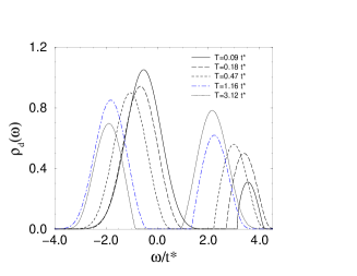
Figure 8: Interacting density of states plotted versus $\omega$ for $U=4$, $E_{f}=-0.5$ ($T_{v}=0.14$), and for various temperatures, as indicated in the figure.

The intraband optical conductivity is determined by an integral of the spectral function (Pruschke, et al., 1995) as

$$\sigma(\omega)=\sigma_{0}\int d\epsilon\rho(\epsilon)\int d\nu\frac{f(\nu)-f(\nu+\omega)}{\omega}A(\epsilon,\nu)A(\epsilon,\nu+\omega),$$ (101)

where $A(\epsilon,\nu)=-\frac{1}{\pi}{\rm Im}~{}[1/(\nu+\mu-\Sigma(\nu)-\epsilon)]$ is the spectral function. The result for $\sigma(\omega)$ obtained in such a way is plotted in Fig. (9) as a function of frequency, for several temperatures. Above $T_{v}$, we observe a reduced Drude peak around $\omega=0$ and a pronounced high-frequency peak around $\omega\simeq U$. The shape of $\sigma(\omega)$ changes completely across $T_{v}$. Below $T_{v}$ the Drude peak is fully developed and there is no high-energy (intraband) structure. However, if the renormalized f-level is close to $\mu$, the interband d-f transition could lead to an additional mid-infrared peak.

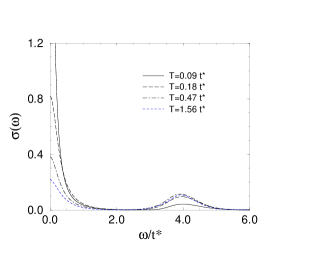
Figure 9: Optical conductivity plotted versus $\omega/t^{*}$ for various temperatures. The $U$, $E_{f}$, and $T_{v}$, are the same as in Fig. (8).

If we estimate the f-d correlation in YbInCu₄ from the 8000 $cm^{-1}$ peak in the optical conductivity data(Garner et al., 2000), we obtain the experimental value $U\simeq 1$ eV. Together with $T_{v}=42$ K (Sarrao et al 1999) this gives the ratio $U/T_{v}\simeq 200$. If we take $U=4$ and adjust $E_{f}$ so as to bring the theoretical value of $T_{v}$ in agreement with the thermodynamic and transport data on YbInCu₄, we get a high-frequency peak in $\sigma(\omega)$ at about 8000 $cm^{-1}$, 6000 $cm^{-1}$, and 1500 $cm^{-1}$, for $E_{f}=-0.75$, $E_{f}=-0.7$, and $E_{f}=-0.5$, respectively.

From the preceding discussion it is clear that the Falicov-Kimball model captures the main features of the experimental data for YbInCu₄ and similar compounds. However, our calculations describe much better the doped Yb systems with broad transitions, than those compounds which show a first-order transition. The numerical curves can be made sharper (by adjusting the parameters) but they only become discontinuous in a narrow parameter range. Our results indicate that the temperature- and field-induced anomalies are related to a metal-insulator transition, which is caused by a large FK interaction and triggered by the temperature- or the field-induced change in the f-occupancy.

Summary and outlook

We studied the static and dynamic correlation functions of the infinite–dimensional FK model by an equation-of-motion method. The exact solution (Brandt and Mielsch, 1989; Brandt and Urbanek, 1992) has been presented for the model with an arbitrary number of electrons, and for a $(2s+1)$–fold degenerate d-state and a $(2S+1)$–fold degenerate d-state. In the large-U limit, and for a range of parameters, the spin-one-half model exhibits a transition from a high-temperature semiconductor or a semimetal, with well defined f-moments, to a low-temperature Pauli metal. The static and dynamic correlation functions show many similarities with the experimental data on valence fluctuating Yb-compounds, and perhaps on SmB₆, but the crossovers calculated for the spin-one-half model are less sharp than what is seen in the experimental data. We believe, the sharpness of the transition in Yb–compounds is due to the large entropy change, when Yb ions switch from the magnetic $4f^{13}$ configuration (with a 14–fold degenerate f-hole in the $J=7/2$ spin-orbit state) to a non-magnetic $4f^{14}$ configuration. The model with a 14-fold degenerate f-state and a 2-fold degenerate d-state can easily be solved by the methods explained in this paper, and we expect to see a much sharper transition there. The numerical analysis of such a model, and the study of the correlation functions for various values of the ratio $(2S+1)/(2s+1)$, will be the subject of subsequent work.

A more serious difficulty with the FK model is that it neglects the quantum fluctuations of the f-state and considers only statistical fluctuations. That is, the lifetime of an f-state is assumed to be infinite, and the width of the f-spectrum arises only because the f-electrons couple to density fluctuations in the conduction band. Thus, the valence transition in the FK model is accompanied by a substantial change in the f-occupancy, and the loss of the magnetic moment is associated with the loss of f-holes. In real materials, the loss of the local moment seems to be due to quantum fluctuations and lifetime effects, rather than to the disappearance of the f-holes, The description of the quantum valence fluctuating ground state would have to consider the hybridization between the f- and d-states, and that would require a periodic Anderson model with an additional FK interaction. The EOM method elaborated in this paper does not produce the solution for such a generalized model.

The actual situation pertaining to Yb ions in the mixed-valence state might be quite complicated, since one must consider an extremely asymmetric limit of the Anderson model, in which the ground state is not Kondo-like, there is no Kondo resonance, and there is no single universal energy scale which is relevant at all temperatures(Krishnamurti et al., 1980). We speculate that the periodic Anderson model with a large FK term will exhibit the same behavior as the FK model at high temperatures. Indeed, if the conduction band and the f-level are gapped, and the width of the f-level is large, then the effect of the hybridization can be accounted for by renormalizing the parameters of the FK model. On the other hand, if the low-temperature state of the full model is close to the valence-fluctuating fixed point with the conduction band and hybridized f-level close to the Fermi level, then the likely effect of the FK correlation is to renormalize the parameters of the Anderson model.

This picture is borne out from our examination of the spontaneous hybridization for the spinless FK model on the Bethe lattice. We find that as $T$ is lowered the system seems to have a logarithmic divergence in the spontaneous hybridization susceptibility at $T=0$. Normally we cannot reach such a phase because the system will have a phase transition to either a phase separated state or a charge-density wave, but we can tune the system so that it remains in a classical intermediate valent state down to $T=0$. When this occurs, effects of even a small hybridization will take the system away from the FK fixed point at low enough $T$ and hybridization can no longer be neglected.

Appendix

The matrix elements in Eqs. (88) and (89), which are used to calculate the determinant in Eq. (90) for the f-propagator, are given by the expressions,

$$M_{(n\neq m)} = \xi_{0}A_{nm}+(\xi_{0}-1)B_{nm}$$ (102)

$$M_{(n,n)} = \xi_{0}C_{nn}+(\xi_{0}-1)D_{nn}$$ (103)

where $\xi_{0}=1/(1+e^{U\tau-\beta\mu})$, and

$$A_{mn} = \frac{1}{i(\omega_{m}-\omega_{n})(i\omega_{m}+\mu-U)}-\frac{e^{i\tau\omega_{n}+\mu\tau-\beta\mu}}{(i\omega_{m}+\mu)(i\omega_{n}+\mu)}$$

$$+ \frac{(e^{-(i\omega_{m}+\mu)\tau}+e^{-\beta\mu})(e^{(i\omega_{n}+\mu)\tau}-e^{U\tau})}{(i\omega_{m}+\mu)(i\omega_{n}+\mu-U)}$$

$$- \frac{1}{i(\omega_{m}-\omega_{n})(i\omega_{n}+\mu)}+\frac{e^{-i(\omega_{m}-\omega_{n})\tau}}{i(\omega_{m}-\omega_{n})(i\omega_{m}+\mu)}$$

$$+ \frac{e^{-(i\omega_{m}+\mu)\tau}[i(\omega_{m}-\omega_{n})e^{U\tau}-(i\omega_{m}+\mu-U)e^{(i\omega_{n}+\mu)\tau}]}{i(\omega_{m}-\omega_{n})(i\omega_{m}+\mu-U)(i\omega_{n}+\mu-U)}\left.\right.$$

$$B_{mn} = \frac{-1}{i(\omega_{m}-\omega_{n})(i\omega_{n}+\mu-U)}-\frac{e^{-i(\omega_{m}-\omega_{n})\tau}}{i(\omega_{m}-\omega_{n})(i\omega_{n}+\mu)}$$

$$- \frac{e^{i\omega_{n}\tau}(e^{-i\omega_{m}\tau}-e^{(\mu-U)\tau})-e^{\beta\mu}(e^{-(i\omega_{m}+\mu)\tau}-e^{-U\tau})}{(i\omega_{m}+\mu-U)(i\omega_{n}+\mu)}$$

$$+ \frac{i\omega_{n}+\mu-i(\omega_{m}-\omega_{n})e^{\beta\mu-(i\omega_{m}+\mu)\tau}}{i(\omega_{m}-\omega_{n})(i\omega_{m}+\mu)(i\omega_{n}+\mu)}$$

$$+ \frac{e^{-i(\omega_{m}-\omega_{n})\tau}[i\omega_{n}+\mu-U+i(\omega_{m}-\omega_{n})e^{(i\omega_{m}+\mu-U)\tau}]}{i(\omega_{m}-\omega_{n})(i\omega_{m}+\mu-U)(i\omega_{n}+\mu-U)}$$

$$C_{nn} = \frac{(i\omega_{n}+\mu-U)\tau-1+e^{-(i\omega_{n}+\mu-U)\tau}}{(i\omega_{n}+\mu-U)^{2}}$$

$$+ \frac{1-e^{-(i\omega_{n}+\mu-U)\tau}-e^{-\beta\mu}(e^{(i\omega_{n}+\mu)\tau}-e^{U\tau})}{(i\omega_{n}+\mu)(i\omega_{n}+\mu-U)}$$

$$+ \frac{(i\omega_{n}+\mu)(\beta-\tau)-1-e^{-\beta\mu+(i\omega_{n}+\mu)\tau}}{(i\omega_{n}+\mu)^{2}}$$

$$D_{nn} = \frac{-(i\omega_{n}+\mu-U)\tau-1+e^{(i\omega_{n}+\mu-U)\tau}}{(i\omega_{n}+\mu-U)^{2}}$$ (107)

$$+ \frac{1-e^{(i\omega_{n}+\mu-U)\tau}-e^{\beta\mu}(e^{-(i\omega_{n}+\mu)\tau}-e^{-U\tau})}{(i\omega_{n}+\mu)(i\omega_{n}+\mu-U)}$$

$$+ \frac{(i\omega_{n}+\mu)(\tau-\beta)-1-e^{\beta\mu-(i\omega_{n}+\mu)\tau}}{(i\omega_{n}+\mu)^{2}}$$

These expressions generalize the matrix elements obtained in (Brandt and Urbanek 1992) for the system with electron-hole symmetry. We checked, that for $\mu=U/2$ our expressions agree with those of Brandt and Urbanek (1992) for $m\neq n$, but we find a slight inconsistency for the case $m=n$. The formulae given here, and those given by Brandt and Urbanek agree only if the minus sign in front of the $i\omega_{m}$ term which appears in the numerator of the first line of the expression for $M_{(m,m)}$ in Brandt and Urbanek (1992) is replaced by a plus sign.

References

- [1] U. Brandt and C. Mielsch, Z. Phys. B 75, 365 (1989);
- [2] U. Brandt and M. P. Urbanek, Z. Phys. B 89, 297 (1992).
- [3] G. Czycholl, Phys. Rev. B 59, 2642 (1999).
- [4] S. Elitzur, Phys. Rev. D 12, 3978 (1975).
- [5] L. M. Falicov and J. C. Kimball, Phys. Rev. Lett. 22, 997 (1969).
- [6] P. Farkasovšký, Z. Phys. B 104, 553 (1997); Phys. Rev. B 59, 9707 (1999).
- [7] J. Freericks and V. Zlatić, Phys. Rev. B 58, 322 (1998); V. Zlatić and J. Freericks, in Proc. NATO ARW Conference, Bled 2000, edited by P. Prelovsek, S. Sarkar, J. Bonca (North-Holland, Amsterdam, 2001).
- [8] J. K. Freericks and R. Lemanski, Phys. Rev. B 61, 13438 (2000).
- [9] S.R. Garner, J.N. Hancock, Y.W. Rodriguez, Z. Schlesinger, B. Bucher, Z. Fisk, and J.L. Sarrao, Phys. Rev. B 62 (2000) R4778.
- [10] G Guntherodt, W. A. Thompson, F. Holtzberg and Z. Fisk, in Valence Instabilities, edited by P.Wachter and H. Boppart (North-Holland, Amsterdam, 1982).
- [11] L.P. Kadanoff and G. Baym, Quantum Statistical Physics (W. A. Benjamin, Menlo Park, CA, 1962).
- [12] H. B. Krishnamurti, J. W. Wilkins, and K. G. Wilson, Phys. Rev. B 21, 1044 (1980).
- [13] W. Metzner and D. Vollhardt, Phys. Rev. Lett. 62, 324 (1989).
- [14] T. Portengen, Th. Oestreich and L.J. Sham, Phys. Rev. Lett. 76, 2284 (1996); Phys. Rev. 54, 17452 (1996).
- [15] Th. Pruschke, M. Jarrell, and J. K. Freericks, Adv. Phys. 44 187 (1995).
- [16] J.L. Sarrao, Physica B, 259&261, 129 (1999).
- [17] Q. Si, G. Kotliar, and A. Georges, Phys. Rev. B 46, 1261 (1992).
- [18] V. Subrahmanyam and M. Barma, J. Phys. C 21, L19 (1988).
- [19] P.Wachter and G. Travaglini, J. Mag. Mat. Mater. 47-48, 423 (1985).
- [20] Woonki Chung and J. K. Freericks, Phys. Rev. Lett. 84, 2461 (2000).