Helium nanodroplets and trapped Bose-Einstein condensates
as prototypes of finite quantum fluids
Abstract
Helium nanodroplets and trapped Bose-Einstein condensates in dilute atomic gases offer complementary views of fundamental aspects of quantum many-body systems. We discuss analogies and differences, stressing their common theoretical background and peculiar features. We briefly review some relevant concepts, such as the meaning of superfluidity in finite systems, the behavior of elementary excitations and collective modes, as well as rotational properties and quantized vorticity.
I Introduction
Helium clusters have been the object of a rather extensive investigation in the last two decades. They are becoming even more interesting nowadays, due to the improved accuracy of recent experiments where several properties of the clusters are characterized by using dopant atoms and molecules as efficient probes [1]. In 1995, the observation of Bose-Einstein condensation (BEC) in ultracold vapors of alkali-metal atoms [2, 3, 4] opened another active field of research. This event is seemingly disconnected from the physics of helium clusters. The framework in which BEC was initially investigated is a mix of atomic physics and quantum optics, while helium clusters are a typical subject of condensed matter and chemical physics. As a consequence, some of the key words used to interpret the first experimental results on BEC (like order parameter, coherence length, phase coherence, elementary excitations, and others) had sometimes different meaning in the two communities. However, as soon as trapped condensates were sufficiently characterized, by using the Gross-Pitaevskii theory as a starting point, most of the physics behind these systems appeared to be strongly connected with the physics of superfluids. One can even say that helium droplets and trapped atomic gases correspond to two limiting cases of the same system since they are, respectively, examples of very dense and dilute finite-sized quantum fluids. Despite the different type of confinement (self-binding for helium droplets and external trapping for atomic gases) these systems belong to the same conceptual framework, possibly based on a common language.
A quantum fluid is a system of many interacting particles for which one can locally define both a density and a velocity field, whose behavior is strongly affected by quantum correlations. An example of these quantum effects is the zero point motion, which is crucial in determining the typical lengthscales for density modulations, like the surface thickness at the fluid boundaries, the core size of a vortex, the size of soliton-like structures. Another important effect is the fact that the fluid, or part of it, moves with a non-dissipative and irrotational velocity field, which means that the system is superfluid. These and other features can be associated with the existence of an order parameter. Qualitatively, as the particles are cooled down to enough low temperatures their de Broglie wavelength becomes larger than their average separation, so that they loose their individual identity. In the case of bosons, they can be treated as components of a single “macroscopic wave function”. The concept of order parameter is the appropriate tool to implement this qualitative idea.
The temperature at which these effects occur is generally very low, so that the fluid actually freezes before reaching this regime. In the case of liquid 4He, the light atomic mass allows the system to remain liquid down to zero temperature and the system becomes a quantum fluid for temperatures lower than about K. In the case of trapped condensates, vapors of alkali-metal atoms are kept in a metastable gas-phase down to temperatures of the order of tens of nanokelvin, where quantum effects becomes dominant. The fact that these systems are in a metastable configuration is compatible with the existence of a kinetic equilibrium which is ensured by two-body elastic collisions. The transition to the thermodynamic equilibrium, given by the crystal phase, is instead driven by three-body recombinations, which are however rare events in very dilute samples and take place on a relatively long time scale.
When the fluid becomes a quantum fluid the type of quantum statistics is also crucial and one can find either a Fermi or a Bose fluid with very different properties. Liquid 3He is the fermionic counterpart of 4He, and also alkali-metal atoms with both Fermi and Bose statistics can be trapped and cooled down to the quantum regime. In this brief review, however, we concentrate mainly on Bose fluids.
The paper is organized as follows. First we remind the basic notions of Bose-Einstein condensation, as a common starting point. Then we discuss two opposite limits: a dilute and cold gas, where one can develop a rigorous theory for interacting bosons, and a dense quantum fluid, where more sophisticated many-body techniques are required. Once the theoretical framework is sketched, we finally describe some predicted and/or observed properties of both helium droplets and trapped condensates (critical temperature, ground state, excitations, superfluid effects, etc.) in order to emphasize relevant analogies and differences.
II Bose-Einstein condensation
The intimate link between helium droplets and trapped condensates is the occurrence of Bose-Einstein condensation and the fact that this phenomenon plays a key role in determining most of the properties of both systems.
In the case of noninteracting particles, Bose-Einstein condensation has well established features. The system can be represented by a set of single-particle states of energy , each one occupied by a certain number of particles . At a given temperature , the average occupation numbers are fixed by Bose statistics, resulting in the well known law , where and is the chemical potential. The latter is fixed by the conditions that the total number of particles, , is equal to the sum . For relatively high one finds that this condition is satisfied for , where is the energy of the lowest single-particle state, and the particles are thermally distributed over many states, all of them having of the order of (or, equivalently, much less than ). However, there is no exclusion principle for bosons: many of them can stay in the same state. This happens when the temperature is lowered; when the chemical potential approaches , the occupation of the lowest state becomes a macroscopic number of the order of . This phenomenon is called Bose-Einstein condensation. The critical temperature at which it occurs can be calculated starting from the knowledge of the single-particle Hamiltonian and keeping the appropriate thermodynamic limit .
In the textbook case of a uniform system of free bosons of mass , one increases the volume while keeping the density constant; in this way, one gets the critical temperature [5]
| (1) |
where is the Riemann zeta function and . This result can be rewritten as , where is the thermal de Broglie wavelength. This is a quantitative translation of the qualitative idea mentioned in the introduction: quantum effects become crucial when the de Broglie wavelength becomes larger than the average separation between particles. The same calculations also yields the condensate fraction . At all particles are in the state, that is, the system is fully condensed. This state has a uniform density and is characterized by having zero momentum; for this reason, one often speaks of condensation in momentum space. It is important to stress here that, when applied to liquid 4He ( and being the atomic mass and the liquid density, respectively), Eq. (1) gives a transition temperature reasonably close to , i.e., the temperature at which helium becomes superfluid. This very simple and striking result marked the beginning of the theory of superfluids, starting from the pioneering work of Fritz London [6].
In the case of bosons confined in a spherical harmonic potential , the proper thermodynamic limit is obtained by letting and , while keeping the product constant. In this way the critical temperature is well defined; one finds [7]
| (2) |
and the condensate fraction is . Notice that the different -dependence exhibited by the condensate fraction compared to the uniform case is the consequence of the higher density of states characterizing the harmonic oscillator Hamiltonian. At all particles are in the lowest eigenstate of the harmonic oscillator, namely, . Thus the particle density has the form of a Gaussian and the same is true for the momentum distribution. Differently from the uniform gas, condensation occurs in both real and momentum space. Actually, the occurrence of a sharp peak in the velocity distribution of a cloud of 87Rb atoms, released from a magnetic trap, was the first evidence of Bose-Einstein condensations in these cold gases [2], and the transition temperature was found to be very close to the value predicted by Eq. (2).
Since both liquid 4He and dilute atomic gases are systems of interacting particles, a crucial question concerns the role played by the interaction, that is, whether and how much the interatomic forces modify the properties of Bose-Einstein condensation. Understanding the interplay between quantum statistical and dynamic effects represents the challenging task to achieve both experimentally and theoretically in these quantum many-body systems.
Let us consider a system of particles interacting via a potential and, possibly, with an external field . In principle, one should solve the exact many-body Schrödinger equation or, equivalently, find the eigenvalues of the Hamiltonian
| (3) |
where and are the boson field operators that annihilate and create a particle at the position , respectively. This is a difficult task and we do not discuss here the possible strategies. We only want to emphasize the meaning of Bose-Einstein condensation in terms of a generic solution of the many-body problem. An elegant way [8] consists in writing the one-body density matrix, which is defined as
| (4) |
where the average is taken in the state that one wants to describe. This quantity characterizes the correlations between particles located in different points in space. One can use a complete set of single particle states to explicitly write as a matrix. Then one can diagonalize it, finding eigenstates and eigenvalues. The latter can be interpreted as the occupation numbers associated with each eigenstate. In analogy with the ideal Bose gas, one might expect that below some critical temperature one of these eigenvalues, instead of being of order as all the others, is a number of the order of . The corresponding eigenstate then has a special role in the system, since it is macroscopically occupied. When an interacting system exhibits such a behavior, one says that it is Bose-Einstein condensed.
In the case of a uniform system, the appropriate basis is a set of plane waves, eigenstates of the momentum . If is the number of particles condensed into the lowest energy state, then the density matrix can be written in the form
| (5) |
with . This summation is made over all states except ; for it simply gives the total number of particles with , that is . In the opposite limit, , due to destructive interference between the various phase factors, the function vanishes, while the condensed part of the density matrix remains everywhere constant. This infinite range of the the density matrix (off-diagonal long range order) is also called first order coherence. It is a key consequence of Bose statistics and is the origin of the quantum correlations that are responsible for superfluidity. This is the basic physics behind the superfluid behavior of liquid 4He below . In such a dense system, the effect of the interaction, which is implicitly included in Eq. (5), is very important. Compared to the ideal gas, it changes the features of the phase transition and gives a large depletion of the condensate, being of the order of % even at .
This description can be easily generalized to nonuniform systems. In this case, the contribution to associated with the condensed state is no more a number, but depends on positions. The straightforward generalization of Eq. (5) is
| (6) |
where is of order , while vanishes for large [9]. This is equivalent to say that the bosonic field operator splits in two parts
| (7) |
where the first term is a complex function associated with the macroscopic occupation of the condensate and the second one is the field operator associated with the noncondensed particles. The complex function can be defined as the expectation value of the field operator:
| (8) |
It behaves as a classical field having the meaning of an order parameter, and is often named macroscopic wave function. Its modulus gives the condensate density through , while the phase can be used to define a velocity field through .
Similarly to the case of uniform gases, the fact that the order parameter has a well-defined phase corresponds to assuming the occurrence of a broken gauge symmetry in the many-body system. It is worth noticing that, strictly speaking, in a finite-sized system neither the concept of broken gauge symmetry, nor the one of off-diagonal long-range order can be applied. In fact, the density matrix (6) vanishes for distances of the order of the size of the system so that, in order to make the separation of the condensate and noncondensate components physically meaningful, it is crucial that the lengthscale at which vanishes be much smaller than the size of the system. The condensate wave function can nevertheless be always calculated as the eigenfunction of the density matrix with the largest eigenvalue. A numerical diagonalization of the density matrix was performed, for example, by Lewart et al. [10] in order to estimate the condensate density, , in helium droplets with up to atoms, using a variational Monte Carlo approach.
III Dilute gases and Gross-Pitaevskii theory
The decomposition of the field operator in Eq. (7) is particularly useful when the depletion of the condensate, i.e., the fraction of noncondensed particles, is very small. This happens when the interaction is weak, but also for particles with arbitrary interaction, provided the gas is dilute. In this case, one can expand the Hamiltonian (3) by treating as a small quantity.
In a uniform gas the condensate wave function, , is just a constant and expanding to the lowest order in gives access to the equations for the excited states. This procedure was introduced by Bogoliubov [11], who found an elegant way to diagonalize the Hamiltonian by using simple linear combinations of particle creation and annihilation operators. These are known as Bogoliubov’s transformations and stay at the basis of the concept of quasiparticle, which is one of the most important concepts in quantum many-body theory.
If the gas is nonuniform, the theory has to include an equation for the spatial variation of the condensate, even at the zeroth-order in . A possible strategy consists in writing the Heisenberg equation for the evolution of the field operators, using the Hamiltonian (3):
| (9) |
Then the lowest order is obtained by replacing the operator with the classical field . In the integral containing the atom-atom interaction , this replacement is, in general, a poor approximation when short distances are involved. In a dilute and cold gas, one can nevertheless obtain a proper expression for the interaction term by observing that, in this case, only binary collisions at low energy are relevant and these collisions are characterized by a single parameter, the -wave scattering length, independently of the details of the two-body potential. This allows one to replace in (9) with an effective interaction where the coupling constant is related to the scattering length through . Using this pseudo-potential in Eq. (9) and replacing with , one gets the following closed equation for the order parameter:
| (10) |
This is known as Gross-Pitaevskii (GP) equation [12, 13]. It has been derived assuming that is large while the fraction of noncondensed atoms is small. On the one hand, this means that quantum fluctuations of the field operator have to be small, which is true when , where is the particle density. In fact, one can show that, at the depletion of the condensate is proportional to [5]. On the other hand, thermal fluctuations have also to be negligible and this means that the theory is limited to temperatures much lower than . Within these limits, one can identify the total density with the condensate density .
The stationary solution of Eq. (10) corresponds to the condensate wave function in the ground state. One can write , where is the chemical potential and is real and normalized to the total number of particles, . Then the GP equation becomes
| (11) |
This has the form of a “nonlinear Schrödinger equation”, the nonlinearity coming from the mean-field term, proportional to the particle density . It is worth noticing that the same equation can be obtained by minimizing the energy of the system written as a functional of the density:
| (12) |
The first term corresponds to the quantum kinetic energy coming from the uncertainty principle; it is usually named “quantum pressure” and vanishes for uniform systems.
In the absence of interactions (), the GP equation (11) reduces to the usual single-particle Schrödinger equation. Conversely, when , the mean-field contribution can have an important role in determining the energy and density distribution of the condensate, despite the smallness of the gas parameter . In fact, what matters is the relative weight of the mean-field potential, the kinetic energy, and the external potential. As we will see later on, one can easily find situations where the gas is dilute but strongly nonideal. It is also worth pointing out the key role played by the chemical potential in the GP theory, where the time dependence of the stationary order parameter is fixed by and not by the energy. This is a consequence of the fact that the order parameter is not a wave function and that the GP equation is not a Schrödinger equation in the usual sense of quantum mechanics. From the point of view of many-body theory the order parameter corresponds to the matrix element of the field operator between two many-body wave functions containing, respectively, and particles. This implies that its time dependence is fixed by the factor and hence by the chemical potential rather than by the energy .
The excited states of the condensate, at , can be also calculated starting form the time dependent GP equation (10), by looking for small deviations around the ground state in the form
| (13) |
By keeping terms linear in the complex functions and , Eq. (10) becomes
| (14) | |||||
| (15) |
where . These coupled equations allow one to calculate the eigenfrequencies and hence the energies of the excitations. In a uniform gas, the amplitudes and are plane waves and one recovers the Bogoliubov’s spectrum [11]
| (16) |
where is the wavevector of the excitations. For large momenta the spectrum coincides with the free-particle energy . At low momenta Eq. (16) instead gives the phonon dispersion , where is the sound velocity. This transition between the two regimes occurs when the typical wavelength of the excited states becomes of the order of the so called healing length,
| (17) |
which is a rather important lengthscale for superfluidity. When the order parameter is forced to vanish at some point (by an impurity, a wall, or something else), the healing length is the typical distance over which it recovers its bulk value. In a nonuniform condensate the lowest excitations are not plane waves, but they have still a phonon-like character, in the sense that they involve a collective motion of the condensate, and the transition from phonon-like to single-particle excitations is still an important feature of these systems.
An important point which deserves to be stressed is the existence of a close connection between the dynamics of a condensate, expressed by the GP equation, and the hydrodynamic equations for an irrotational and viscousless fluid. The natural variables for the hydrodynamic description are density and velocity field, which can be related to the modulus and the phase of the order parameter as in Eq. (8). Using these definitions into the GP equation (10) and neglecting the contribution of the quantum pressure, , one gets the two coupled equations
| (18) | |||||
| (19) |
where . These are the continuity and Euler equations for an irrotational and viscousless fluid in the collisionless regime, that is, the hydrodynamic equations for a superfluid at . Neglecting the quantum pressure term in the GP equations means that Eqs. (18) and (19) are valid for macroscopic motions of the condensate, i.e., excitations with wavelength larger than the healing length.
The equations written in this section stay at the basis of most of the theoretical papers recently written on BEC in trapped gases (see [14] for a recent review). Analytical and numerical methods have been developed in order to solve both the stationary and time-dependent Gross-Pitaevskii equation and the results are often in excellent agreement with experiments. On the other hand, the accuracy of the approximations made in deriving the GP equation can be directly tested by performing Monte Carlo simulations, which are exact within statistical errors. For trapped condensates, this has been done in [15] using a Path Integral Monte Carlo method, showing that the stationary GP equation is very accurate for less than about and providing quantitative estimate for the effects of correlations beyond mean-field theory. Such corrections has been also calculated for a uniform hard-sphere Bose gas in [16] using a Green Functions Monte Carlo method.
It is worth mentioning that the theory of weakly interacting Bose gases born well before the observation of BEC in trapped gases, as an attempt to explain the behavior of superfluid helium. In the case of helium, however, the parameter is of the order of , so that the theory looses most of its predictive power.
IV Dense fluids and the quantum many-body problem
When the system is neither weakly interacting nor dilute, the mean-field theory based on Eq. (10) is no more applicable. Quantum correlations beyond mean-field are essential; they can give, for instance, a large depletion of the condensate even at , so that perturbative schemes based on the smallness of in Eq. (7) fail. In order to overcome this obstacle, one can follow two alternative and complementary paths: i) keep the theory at a microscopic level by solving the many-body problem as accurately as possible; ii) develop phenomenological theories, starting from a more macroscopic view of the liquid.
Among the microscopic approaches one can distinguish different strategies depending on the use or non-use of stochastic Monte Carlo procedures. Example of non-stochastic approaches are variational methods and perturbative schemes. Most of them relies on diagram expansion and summation techniques typical of quantum many-body theories. Jastrow-Feenberg [17] wave functions are often used in this context as a starting point. They can be combined with integral equations as in the optimized hypernetted chain (HNC) theory or with perturbative schemes as in the correlated basis function (CBF) theory. The energy minimization within a certain class of variational wave functions can be performed with stochastic techniques as in the variational Monte Carlo (VMC) method. This allows one to include more sophisticated correlations in the trial wave function as, for instance, in the recent Shadow Wave Function theory. Monte Carlo algorithms can finally be used to get exact results with statistical uncertainties. This is the case of approaches like Green’s function MC, Diffusion MC and Path Integral MC, which are powerful, reliable, and computationally demanding. It is not our aim to present an overview of all these theories and calculations. Appropriate references can be found in the various papers where these techniques are applied to helium droplets (see, for instance, [18] and references therein).
Conversely, a problem that deserves to be mentioned at this point is whether it is possible to make a bridge between dilute gases and dense fluids, like helium, within a single theoretical scheme. The recent Variational Monte Carlo calculation by DuBois and Glyde [19] is an interesting effort in this direction. By using a rather simple variational wave function, they evaluated the ground state properties of a trapped Bose gas made of hard-sphere of radius , over a wide range of the parameter . In particular, through the diagonalization of the one-body density matrix, they calculated the condensate fraction showing how it decreases from to about % in bulk, when goes from to the value appropriate for liquid helium, which is about - (the range of the interaction is about - Å, while the density is approximately Å-3). They also pointed out interesting features about its spatial dependence, i.e., the tendency for dense fluids to have larger condensate fraction at the surface where the density is smaller. This enhancement of the condensate was first found in the Variational MC calculations of Ref. [10] in the case of helium droplets.
Phenomenological approaches can also be applied to study dense systems. For confined fluids the simplest one is the liquid drop model. One considers a droplet of constant density within a radius and a sharp surface. Then one can write the energy as a power expansion in (or, equivalently, in power on the number of particles ) taking bulk energy, surface energy, curvature energy, etc., as input parameters. In the limit of large , one can consider the dynamics of these droplets as due to large wavelength, collective motions. Then, it makes sense to use hydrodynamic equations with appropriate boundary conditions in order to get the dispersion of bulk (phonon-like) and surface (ripplon-like) excitations [20, 21]. Several properties of quantum fluid droplets are well predicted by this type of models [22]; what is missing is the accurate description of structures and excitations on a more microscopic scale, i.e., at the level of atomic distances. A step further in this direction is the density functional approach.
In density functional theories at zero temperature, the energy of a system is assumed to be a functional of the particle density . A good starting point for Bose fluid is given by
| (20) |
which is the natural generalization of the Gross-Pitaevskii functional (12). Ground state configurations are obtained by minimizing this energy with respect to the density. This leads to the Hartree-type equation
| (21) |
where acts as a mean field, while the chemical potential is introduced in order to ensure the proper normalization of the density to a fixed number of particles. Equation (21) exhibits a formal analogy with the Gross-Pitaevskii equation (11). The main conceptual difference is that Eq. (21) is an equation for the density and not for the order parameter. While in a dilute gas setting is an excellent approximation, in a correlated system it is meaningless.
The correlation energy incorporates the effects of dynamic correlations induced by the interaction. The fact that this energy is a unique functional of is ensured by the Hohenberg-Kohn theorem [23]. In the case of dilute gases, one simply has , as in Eq. (12). Conversely, since liquid helium is a strongly correlated system, a rigorous derivation of , starting from first principles, is not available. One then resorts to approximate schemes for the correlation energy (see, for instance, Refs. [24, 25] for discussions of this problem from the viewpoint of microscopic many-body theory). A simple but useful approach consists of writing a phenomenological expression for the correlation energy, whose parameters are fixed to reproduce known properties of the bulk liquid. A functional of this type was introduced in Ref. [26, 27] to investigate properties of the free surface and droplets of both 4He and 3He. The correlation energy was written as
| (22) |
where and are phenomenological parameters fixed to reproduce the ground state energy, density and compressibility of the homogeneous liquid at zero pressure, and is adjusted to the surface tension of the liquid. The first two terms correspond to a local density approximation for the correlation energy, while nonlocal effects are included through the gradient correction. Non-locality effects have been included in DFT in a more realistic way by Dupont-Roc et al. [28], who generalized Eq. (22) to account for the finite range of the atom-atom interaction. Further improvements has been added in Ref. [29]. These and other similar functionals have been used for calculations of ground state properties of liquid helium in different geometries (see [30] and references therein).
Dynamical problems can also be faced with density functionals. On the one hand, one can include in the functional terms which explicitly depends on the current density, as done in [29], thus obtaining two coupled equations for both density and velocity field, which can be numerically solved. Excited states of helium droplets have been obtained in this way [31, 32]; the linearized equations of motions, in this case, correspond to a generalization of the Bogoliubov equations (14)-(15), formally equivalent to the equations of the Random Phase Approximation (RPA) [8] with an effective interaction of phenomenological nature. On the other hand, one can simplify the problem by using a purely hydrodynamic approach, in which the equations of motions for the velocity field are the ones of an irrotational and viscousless fluid, but with the density taken from the minimization of the density functional (20). This viewpoint was chosen, for instance, in Ref. [33] to predict the moment of inertia of doped helium droplets.
V Like and unlike features of helium droplets and trapped condensates
A Temperature
In typical experiments the temperature of 4He droplets is about K [34], as the result of a spontaneous evaporation of the warmest atoms after the formation of droplets in the free jet expansion of helium [35]. This temperature is well below the bulk superfluid transition temperature, K. Path Integral Monte Carlo calculations [36] have shown that even small droplets, with few tens of atoms, are superfluid at this temperature. Moreover, the droplet is cold enough to neglect the thermal activation of excited states. The lowest ones are discretized collective modes (bulk and surface oscillations) which are not significantly populated at K. Thus, for most purposes, helium droplets can be considered as systems.
Trapped condensates can be cooled down to few tens of nK. Again this is the result of evaporation, but here the evaporative cooling process is induced and controlled through an external rf-field which acts on the shape of the confining potential, lowering the edge of the trap and letting the hottest atoms to escape. This cooling process can be continued until most of the thermally excited atoms are removed and, hence, the system can be considered as a condensate at . Differently from helium droplets, the properties of trapped gases can also be studied as a function of , just stopping the evaporative cooling at the desired temperature. In this case, the gas has two components, a condensate and a thermal cloud, and the Gross-Pitaevskii theory of section III has to be generalized to properly include the thermal component. In the following, however, we restrict the analysis to [37].
B Ground state
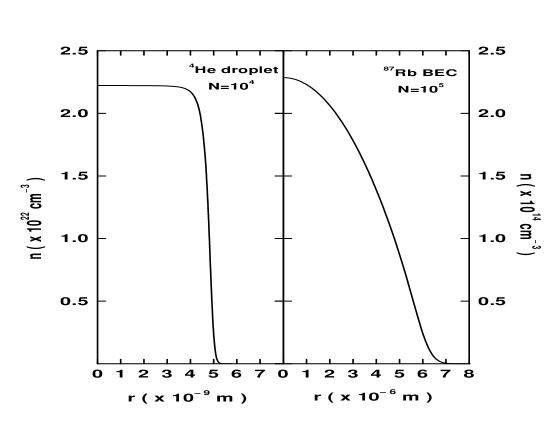
Let us consider a typical helium cluster of - atoms. In its ground state, it is a self-bound liquid droplet with a rather flat density distribution, the central density being close to the one of the uniform liquid in the limit of zero pressure, i.e., Å-3 (see Fig.1). Assuming the droplet to have constant density and sharp surface, its radius would be with Å, which gives about to Å, significantly larger than the average atomic distance. Actually, the true density profile has a rather smooth surface due to the large zero point motion of the atoms. The density decreases from the bulk value to zero within about twice the average atomic distance, i.e., about 6 to 9 Å depending on the precise definition of the surface thickness (see [38] and references therein). The thickness of the surface region is comparable to the droplet radius for of the order of or less, but even for larger droplets the diffuseness of the surface can play a significant role. For instance, it makes the average density of the droplet lower than the bulk liquid value and hence the atoms are less bound to the droplet than to the uniform liquid. As already said, one can reasonably use the liquid drop model to express the energy per particle as a function of :
| (23) |
where K is the volume coefficient, i.e. the energy per particle in the bulk liquid (in the limit of zero temperature and zero pressure), and the next terms are surface and curvature energies. This type of formulae are frequently used to fit the numerical results of ground state calculations.
The density distribution of a pure helium droplet is determined by the balance of the kinetic energy, associated with the zero-point motion of the atoms, and the potential energy due to atom-atom interaction. One can also produce density modulations in the droplets by picking up a foreign atom or molecule, acting as an external potential in which helium atoms readapt. This is, however, a local effect, in the sense that the main changes in the density distribution are limited to the first layers of atoms around the impurity.
Differently from helium droplets, trapped condensates are not self-bound. They are produced and maintained in an external confining harmonic potential, of the form [39]. If this potential is switched-off, the condensate freely expands.
The density distribution of a trapped gas is determined by the balance of three energy contributions given in Eq. (12). Since the sign of the interaction energy is fixed by the scattering length , one may have either a repulsive or attractive mean-field potential, for positive and negative , respectively. The case of negative is very interesting for several reasons but it is not suitable for a comparison with helium. In fact, a uniform gas of atoms with negative is unstable; it has negative pressure and it lowers its energy by collapsing into separate regions of high density. In a trap, quantum pressure can prevent this collapse, at least below some critical density [14], but such metastable condensates have no counterpart in the uniform limit, differently from the case of liquid helium and of trapped condensates with positive .
If the atoms were not interacting () the condensate would have the form of the lowest single-particle state in the harmonic potential, i.e, a Gaussian having a width . In actual condensates, with , the repulsion between atoms tends to lower the central density, thus increasing the condensate width. The equilibrium configuration is again fixed by the balance between , and . It turns out that for (Thomas-Fermi limit) the density in the central part is so smooth that the quantum pressure is negligible compared to both and . In this case, the GP equation (11) simply gives , that is, a density having the form of an inverted parabola. In the same limit, one can easily calculate the energy per particle,
| (24) |
which contains both the harmonic potential parameters and the scattering length. Only in a narrow region at the surface, where the density vanishes, the interaction term becomes small and the density profile is determined by the balance between quantum pressure and external potential [40]; it deviates from the inverted parabola and goes smoothly to zero. This surface region gives a logarithmic correction to the Thomas-Fermi energy (24), of the form . An example is shown in Fig.1, where one can see how the external potential affect the overall shape of the condensate (right panel), in contrast with the self-bound helium droplet (left panel).
At present, several types of condensates are available in different labs (different geometries and atomic species). Let us consider a common situation of a condensate made by - atoms of sodium or rubidium, in a trap with - Hz. The width of the condensate can be several m, but wider condensates, up to m, have been obtained in anisotropic traps. The scattering length is of the order of a few nm and the ratio is about , so that ; thus the density profile is very well represented by an inverted parabola with a thin surface region. The size of the system is much larger than the average interatomic distance, of the order of m, as happens for large helium droplets. The central density is of the order of - cm-3, so that is less than , which ensures the applicability of Gross-Pitaevskii theory.
The relevant lengthscales are summarized in Table I for a 4He droplet with atoms and a trapped condensate of atoms of 87Rb. One notes that the only difference in , and is a common rescaling, from nm (helium) to m (trapped BEC). This is not true for , which is of the same order of in the dense fluid and much smaller than in the dilute gas.
A direct consequence of the very different values of for the two systems in Fig.1 is that the total density plotted in the right panel can be also identified with the condensate density, since quantum depletion is negligible (less than %), while the same is not true for helium. In the latter case, the condensate density is expected to be about % of the total density in the inner part of the droplet, increasing to a maximum value at the surface where the system is more dilute [10] (see also [41] for a recent discussion).
C Excitations
A peculiar feature of Bose superfluids is that their excitations at low energy correspond to collective modes, which can be described as fluctuations of the order parameter. This happens when their wavelength is larger than the healing length.
For uniform and dilute gases, the spectrum of excitations is given by the Bogoliubov result (16), which is phononic at low and single-particle at high . Low excitations are phonons even in liquid helium, with sound velocity m/s. However, since the fluid is dense and highly correlated, the interpolation between the phononic and single-particle regimes is more subtle. The phonon branch reaches a maximum at Å-1 and then forms a rather deep minimum at Å-1, with energy K. The excitations near this minimum, whose dispersion is approximately parabolic, are called rotons. Their wavelength is of the order of the interatomic distances and slightly larger than the healing length, so that they still have collective character, but are related, roughly speaking, to a tendency to local order on the atomic scale.
Helium droplets and trapped BEC have a finite radius . As a consequence, the spectrum is discrete and the excited states have to be classified according to the number of radial nodes, , and the angular momentum quanta ( and , if the system is spherical). The discretization is particularly important for the lowest energy excitations, whose wavelength is comparable with , and correspond to oscillations of the whole system.
An example of collective mode is the state with and , which is a purely compressional oscillation (monopole, or breathing mode). By keeping and increasing , one finds density oscillations in the radial direction having wavelength smaller than . If is large, so that the wavelength becomes much smaller than but still larger than (see Table I), these modes can be thought as stationary states of bulk excitations (phonons and/or rotons) which propagate radially and reflect at the surface. For large , these discretized states approach a continuum and the spectrum becomes closer and closer to the one of a uniform system, namely, the phononic Bogoliubov dispersion in dilute gas and the phonon-roton branch in liquid helium.
Another interesting class of excitations is the one with and . These modes correspond to shape oscillations, or surface excitations, because the motion is mainly concentrated near the surface, the latter being displaced in and out periodically. The lowest one is the quadrupole deformation, . By increasing one gets shape oscillations with more nodes in the angular direction, that is, surface waves with shorter wavelength. In the absence of external confinement as in helium droplets, and for large , these states approach the collective waves of the liquid-vapour interface (ripplons), having dispersion , where is the surface energy and is the wavevector parallel to the surface. In the case of trapped gases the dispersion is instead given by the law , where is the trapping harmonic force calculated at [42].
How can these collective states be excited and observed? In trapped condensate the answer is simple: one can modulate the external potential in order to force oscillations in the system in a classical way. With this method, one has already observed monopole, dipole, quadrupole modes, as well as higher multipolarities [43, 44, 45]. Their frequency is measured with great accuracy and the agreement with theory is very good. The theoretical work basically corresponds to the numerical solution of the Bogoliubov-like equations (14)-(15). In the Thomas-Fermi limit, , one can also obtain analytic results by linearizing the hydrodynamic equations (18)-(19) [46]. In spherical traps one obtains the dispersion relation , which can be compared with the spectrum of noninteracting particles in the same harmonic potential, [47].
Phonon-like excitations with wavelength smaller than the condensate size can also be produced. For instance, one can suddenly switch-on a narrow laser beam, focused in the center of the trap. An optical dipole force acts on the atoms generating a wavepacket of excitations which then moves throughout the condensate as a sound wave. The velocity of this sound wave has been measured in [48], finding good agreement with the prediction of Bogoliubov theory. Phonon-like excitations have been also generated in light-scattering experiments [49].
Driving collective excitations in helium droplets, in a controllable way, is much less simple, since there is no confining potential to play with. However, one can produce and probe excitations by picking up impurities. A foreign atom or molecule, laying inside the droplet or at the surface, can be excited with a laser and this excitation may couple to the internal degrees of freedom of the droplet. This mechanism is at the basis of the so-called depletion method: a photon absorbed by an embedded impurity causes a transfer of energy from the impurity to the droplet via the creation of excitations. The latter eventually exchange their energy with atoms at the surface, letting them to evaporate through a quantum evaporation process. Thus, by monitoring the droplet beam with a mass spectrometer, one detects the spectroscopic transitions of the impurity which, in turn, contain information about the droplet itself [50]. This process has some interesting analogies with the quantum evaporation experiments in bulk helium [51], where the initial bunch of excitations (phonons and/or rotons) is produced by a heater immersed in the liquid, while the evaporated atoms are collected at a bolometer above the surface. There are also significant analogies with the sound propagation experiment in a trapped condensate [48], where the “heater” is represented by the laser beam. In this case, if the trap is kept on, phonons do not evaporate atoms, but they may exchange energy with single-particle states in the outer part of the condensate.
An example of how the superfluid environment affects the spectrum of embedded impurities is the observation of the phonon wing in the electronic excitation spectrum of a glyoxal (C2H2O2) molecule in helium droplets with about atoms [52]. The observed features were found to be consistent with the existence of a phonon-roton spectrum of excitations inside the liquid droplet, with no low-lying single-particle excitations, as expected for a Bose superfluid. Theoretical calculations have also shown that, for droplets of this size, the discretized spectrum of collective excitations closely resembles the continuum of phonons and rotons of bulk liquid [21, 31, 53, 54].
Not all impurities are bound inside helium droplets; some prefer to stay at the surface. In this case, they can be sensitive to surface modes. For large droplets, theoretical calculations show that the spectrum of these excitations, with , is close to the one of collective waves on a planar helium-vacuum interface (ripplons) [55]. This also ensures that the liquid drop model (LDM) is accurate enough for many purposes. For example, using the liquid drop model for the excited states, together with a statistical method for the evaporation rate, the typical temperature of helium clusters in a supersonic beam was calculated in Ref. [35]. The predicted values, for both 3He and 4He droplets, were later found to agree with experiments [34], so providing an indirect insight into the spectrum of surface excitations.
The fact that in a uniform superfluid system single-particle excitations are not allowed to exist below the low-energy collective modes is at the basis of the well known “Landau criterion”. This says that, in order to create excitations in a superfluid by moving an impurity, one has to overcome some critical velocity, which is fixed by the spectrum of the excited states of the system. This follows from the conservation of energy and momentum. In a uniform system the critical velocity is , where is the energy of an excitations carrying momentum [56]. In liquid helium such a critical velocity has been the object of a longstanding investigation, involving the structure of the phonon-roton branch and the nucleation and dynamics of quantized vortex lines and rings. Recently an experiment was realized to test the applicability of the Landau criterion to helium droplets [57]. By studying low energy collisions of 4He and 3He atoms on 4He droplets, the authors found that 3He has a significant probability to fly throughout the droplet without dissipation of momentum and energy, and they interpreted this as a consequence of the Landau criterion. The existence of analog critical velocities in dilute condensates is also currently investigated. In Ref. [58] an external potential (a laser beam) is used to produce a hole in a trapped Bose-Einstein condensate and this hole is moved back and forth at variable velocity, playing the role of a massive impurity. Theoretical interpretations in terms of the Landau criterion have been already presented in Refs. [59, 60].
D Rotations and moment of inertia
When a system is described by an order parameter of the form (8), a crucial consequence is the irrotationality of the superfluid flow, whose velocity field is given by , the phase playing the role of velocity potential. This is a fundamental feature characterizing the superfluid motion, which applies to both liquid helium and dilute condensates. In this connection, it is worth recalling that, despite the fact that in a strongly correlated superfluid differs from the density , the current associated with the superfluid velocity , at , is still given by . The irrotationality of the superfluid flow has important manifestations like, for instance, the peculiar behavior of the moment of inertia and the occurrence of quantized vortices.
The moment of inertia can be defined as the response, , to a rotating field of the form , where is the third component of the angular momentum operator. By rewriting the equations of hydrodynamics (18)-(19) in the frame rotating with angular velocity , one gets the irrotational moment of inertia
| (25) |
where is the classical rigid value. This reduction of the moment of inertia compared to the rigid value was observed in liquid helium in the 60’s, so providing independent measurements of superfluid density [61]. In both helium droplets and trapped condensates, however, the direct measurement of is not feasible and, consequently, the determination of requires more subtle probes.
A suitable solution for trapped condensates is provided by the fact that, if the trap is deformed, the quadrupole and rotational degrees of freedom are coupled. This is well understood by taking a trap with frequencies and considering the exact commutation relation , which explicitly points out the link between the angular momentum operator and the quadrupole operator . Since the quadrupole variable can be easily excited and imaged in these systems, one can use it to get information on . A successful method consists in preparing a deformed condensate, whose shape at equilibrium is an ellipsoid with different major axis along and , and suddenly rotating the magnetic trap by a certain angle around . The condensate then responds with an oscillation of its major axis in the -plane around the new equilibrium orientation. This is called scissors mode. Using the hydrodynamic equations for an irrotational superfluid, one predicts the oscillation frequency [62], which is different from the result of a classical gas, . The explicit relationship between the scissors mode and the moment of inertia was derived in [63]. Recent experiments [64] have nicely confirmed these predictions. The observed moment of inertia clearly points out the superfluid nature of these condensates.
In helium droplets, rotations can be induced and probed by acting on embedded impurities, namely, by studying their rotational transitions. Molecules like SF6, OCS, HCN, and many others have been already used (see Ref. [65] for a recent review). Their spectrum inside the helium droplet exhibits sharp rotational lines, as those of free molecules, except for a different value of their moment of inertia. The sharpness of the spectrum is already a signature that the cold matrix around the molecule is superfluid. A nonsuperfluid matrix would smear the spectrum so much that it could not be resolved; a demonstration of this effect has been given in Ref. [66] by replacing 4He (super) with a variable amount of 3He (normal). In this case, the 3He component provides the low-lying single-particle (particle-hole) excitations which cause the broadening of the rotational spectrum of the molecule. On the other hand, the fact that the observed moment of inertia is systematically larger than the one of the free molecule (up to a factor 4 or 5 for some of them) is an interesting consequence of a dynamical coupling between the rotational degrees of freedom of the molecule and of the superfluid environment. Many experimental results are now available, but there are still open questions in their theoretical interpretation [33, 65, 67, 68]. One of the main problems is that the coupling between the rotor and the superfluid occurs on a microscopic lengthscale, comparable with both the interatomic distances and the healing length. On this scale, one is not fully ensured about the applicability of the superfluid hydrodynamic equations and/or of definitions of “local” superfluid and normal densities.
E Rotations and quantized vortices
Quantized vortices are striking manifestations of superfluidity. In liquid helium they have been the object of a longstanding investigation, starting from the pioneering ideas of Onsager and Feynman [69] (see [70] for a detailed overview). As soon as BEC was observed in trapped gases, the search for quantized vortices in these new systems became one of the primary goals. Recently, single vortices and arrays of vortices have been obtained with different techniques: by “phase imprinting” [71], by using a laser beam “stirrer” [72], by rotating the magnetic trap [73], and by rotating the thermal cloud during the evaporative cooling process [74]. Conversely, quantized vortices have not yet been observed in helium nanodroplets.
The quantization of the circulation in a superfluid directly follows from the assumption that the order parameter (8) must be single-valued. Hence, the increment of the phase over any closed path must be zero or an integral multiple of . If the superfluid fills a simply-connected region, the irrotationality of the velocity field () strictly implies that the increment is zero, and the superfluid can not rotate at all. In certain conditions, however, the fluid may prefer to develop vortical lines, where the superfluid density vanishes. The increment of around these lines can be an integral multiple of and this implies that the circulation is an integral multiple of the quantum .
The density distribution and the velocity field around a single rectilinear vortex line with circulation can easily be calculated in the case of dilute gases by using the Gross-Pitaevskii theory. In fact, a quantized vortex can be regarded as a stationary solution of Eq. (10) of the form
| (26) |
where is the azimuthal angle, is the distance from the -axis, and is a real function obeying the equation
| (27) |
The velocity field associated with the order parameter (26) takes the form where is the unit vector along . It satisfies the irrotationality constraint everywhere except along the vortical line and gives rise to a total angular momentum given by . The centrifugal term in Eq. (27) originates from the peculiar behaviour of the velocity field of the vortical configuration. This term is responsible for the vanishing of the condensate density along the -axis. The “core” of the vortex, i.e., the region where the density is depleted, has a radius of the order of the healing length. The density profile and the energy of the vortex can be calculated by numerically solving the GP equation as done, for instance, by us in Ref. [75]. The GP theory can also be used to investigate the nucleation mechanisms and the stability of the vortex configurations (see [76] for a recent review); the theory describes the main features of the vortices observed in trapped BEC and several predictions agree well with the available experimental results.
What makes relatively easy to produce and manipulate vortices in trapped condensate is the possibility to induce rotations in a controllable way by means of laser beams or rotating traps. The vortical lines can be directly observed as ”holes” in the density distribution. In fact, although the healing length is usually smaller than the resolution of the optical imaging devices, one can switch-off the confining potential, letting the condensate to expand, and wait till the expanding core is large enough to be observed [77]. Alternatively, one can use the lowest collective modes of the condensate in the trap as a probe of vorticity. For instance, a vortical flow induces a frequency splitting of the two modes with and , which results in a slow precession of the quadrupole shape deformations [78], which is analog to the splitting of the lowest circularly polarized modes of the vibrating wire in Vinen’s “milestone” experiment with superfluid helium [79]. This method has been successfully used to estimate the angular momentum of vortical configuration [80], as well as to detect vortices which are not directly observable because they are bent or tilted [81]. Finally, the phase around a vortex can be also visualized in the form of a dislocation in the fringe pattern produced by the interference of two expanding condensates containing vortex lines [82].
In helium droplets there is no external field to play with and hence vortical configurations are not easy to produce and detect. Vortices might nucleate in the initial stages of the jet expansion, where droplets form and cool down, or in the collisions with molecules in the pick-up scattering chamber; but no quantitative predictions have been given so far about these processes. The stability of a vortex line in a droplet is also an open question. On the basis of purely energetic arguments, a vortex line is not stable since its formation costs a large amount of kinetic energy of the superfluid flow, and the ground state of the droplets is hence always vortex-free [83]. On the one hand, however, if a vortex appears as a metastable state in some dynamical process, then one has to consider also the conservation of both energy and angular momentum in any possible decay mechanism, and one might discover that this state is indeed long-living, despite its large energy, as it has been shown for vortex configurations in trapped condensates. On the other hand, one can use dopant atoms or molecules to pin and stabilize the vortex, as the density functional calculations of Ref. [84] suggest. In this case, the dopant can be used also as a probe of vorticity, through the possible effects of the vortex flow on its rotational spectrum. An interesting perspective in this direction is the possibility to accommodate in the droplet a long chain of linear molecules, such as HCN, as done in Ref. [85]. Such chains are expected to be suitable for the stabilization of a vortex line and, moreover, they can reveal in their spectrum the presence of the vortex flow, like for a vibrating wire in a nanoscale Vinen-like experiment.
VI Conclusions
In this paper we reviewed some properties of both helium nanodroplets and dilute trapped condensates. Our purpose was not to give a systematic and detailed account of the available theories and experiments, but rather to discuss some relevant features which allow one to build a bridge between the two systems. We emphasized the existence of a common theoretical background and of many analogies in the measured properties, as well as of several interesting differences. We mainly used the language of Gross-Pitaevskii and density functional theory because, on the one hand, it represents a very reliable mean-field approach for dilute gases and, on the other hand, density functional approaches has been successfully used also in helium droplets. Of course, the close connections between trapped dilute gases and helium droplets would equally emerge when examined from the viewpoint of more microscopic theories or stochastic Monte Carlo techniques.
Once this bridge is established, one may include most of the recent advances in both fields within a unified perspective, namely, the road towards a deeper understanding of the physics of interacting quantum fluids.
Acknowledgements.
F.D. thanks the Dipartimento di Fisica, Università di Trento for the hospitality. This work is supported by MURST-COFIN2000.REFERENCES
- [1] For a recent overview see, for instance, J.P. Toennies and A.F. Vilesov, Annu. Rev. Phys. Chem. 49, 1 (1998). Up-to-date results are also presented in this issue of J. Chem. Phys.
- [2] M.H. Anderson et al., Science 269, 198 (1995).
- [3] K.B. Davis et al., Phys. Rev. Lett. 75, 3969 (1995).
- [4] C.C. Bradleyet al., Phys. Rev. Lett. 75, 1687 (1995).
- [5] K. Huang, Statistical Mechanics, Second Edition (John Wiley and Sons, New York, 1987).
- [6] F. London, Nature 141, 643 (1938).
- [7] V. Bagnato, D.E. Pritchard and D. Kleppner, Phys. Rev. 35, 4354 (1987).
- [8] Ph. Nozières and D. Pines, The Theory of Quantum Liquids (Addison-Wesley, 1990), Vol. II.
- [9] O. Penrose and L. Onsager, Phys. Rev. 104, 576 (1956).
- [10] D.S. Lewart, V.R. Pandharipande and S.C. Pieper, Phys. Rev. B 37, 4950 (1988).
- [11] N. Bogoliubov, J. Phys. USSR 11, 23 (1947).
- [12] E.P. Gross, Nuovo Cimento 20, 454 (1961) and J. Math. Phys. 4, 195 (1963).
- [13] L.P. Pitaevskii, 1961, Zh. Eksp. Teor. Fiz. 40, 646 (1961) [Sov. Phys. JETP 13, 451 (1961)].
- [14] F. Dalfovo, S. Giorgini, L.P. Pitaevskii and S. Stringari, Rev. Mod. Phys. 71, 463 (1999).
- [15] W. Krauth, Phys. Rev. Lett. 77, 3695 (1996); M. Holzmann, W. Krauth and M. Naraschewski, Phys. Rev. A 59, 2956 (1999).
- [16] S. Giorgini, J. Boronat and J. Casulleras, Phys. Rev. A 60, 5129 (1999).
- [17] E. Feenberg, in Theory of quantum fluids (Academic Press, New York, 1969)
- [18] K.B. Whaley, Int. Rev. Phys. Chem. 13, 41 (1994); D.M. Ceperley, in The Monte Carlo Method in Condensed Matter Physics, edited by K. Binder, Topics in Applied Physics Vol. 71, 2nd ed. (Springer Verlag, Berlin 1995).
- [19] J.L. DuBois and H.R. Glyde, Phys. Rev. A 63, 023602 (2001).
- [20] S. Stringari, in Proc. Int. School E. Fermi, Varenna, CVII Course (North Holland, Amsterdam, 1990).
- [21] M. Casas and S. Stringari, J. Low Temp. Phys. 79, 135 (1990).
- [22] The liquid drop model was first applied to a quantum many body system for the investigation of the structure and dynamics of atomic nuclei, where it played an important role. See A. Bohr and B.R. Mottelson, Nuclear Structure (W.A. Benjamin, N.Y., 1975).
- [23] P. Hohenberg and W. Kohn, Phys. Rev. B 136, 864 (1964).
- [24] E. Krotscheck, Phys. Lett. A 190, 201 (1994).
- [25] A. Griffin, Canadian J. Phys. 73, 755 (1995).
- [26] S. Stringari and J. Treiner, Phys. Rev. B 36, 8369 (1987).
- [27] S. Stringari and J. Treiner, J. Chem. Phys. 87, 5021 (1987).
- [28] J. Dupont-Roc, M. Himbert, N. Pavloff, and J. Treiner, J. Low Temp. Phys. 81, 31 (1990).
- [29] F. Dalfovo, A. Lastri, L. Pricaupenko, S. Stringari, and J. Treiner, Phys. Rev. B 52, 1193 (1995).
- [30] E Cheng, M.W. Cole, W.F. Saam, and J. Treiner, Phys. Rev. Lett. 67, 1007 (1991); F. Dalfovo, Z. Phys. D 29, 61 (1994); A. Lastri et al., J. Low Temp. Phys. 98, 227 (1995); F. Ancilotto, A.M. Sartori, and F. Toigo, Phys. Rev. B 58, 5085 (1998); L. Szybisz. Eur. Phys. J. B 14, 733 (2000); F. Ancilotto, F. Faccin, and F. Toigo, Phys. Rev. B 62, 17035 (2000).
- [31] M. Casas, F. Dalfovo, A. Lastri, Ll. Serra, and S. Stringari, Z. Phys. D 35, 67 (1995).
- [32] M. Barranco and E.S. Hernandez, Phys. Rev. B 49, 12078 (1994).
- [33] C. Callegari, A. Conjusteau, I. Reinhard, K. K. Lehmann, G. Scoles, F. Dalfovo, Phys. Rev. Lett. 83, 5058 (1999); 84, 1848(E) (2000).
- [34] M. Hartmann, R.E. Miller, J.P. Toennies, and A.F. Vilesov, Phys. Rev. Lett. 75, 1566 (1995).
- [35] D.M. Brink and S. Stringari, Z. Phys. D 15, 257 (1990).
- [36] P. Sindzingre, M.L. Klein and D.M. Ceperley, Phys. Rev. Lett. 63, 1601 (1989).
- [37] We note on passing that one of the relevant topics about trapped gases is the kinetics of the formation of the condensate during the evaporation process. This might have significant analogies with the formation of the superfluid phase (and the condensate) in helium droplets in the first stages of the evaporative cooling in the free jet expansion. From the conceptual viewpoint, this process is interesting and non-trivial, both for helium and trapped condensates.
- [38] J. Harms, J.P. Toennies and F. Dalfovo, Phys. Rev. B 58, 3341 (1998).
- [39] We only consider the case of isotropic confinement, even though the traps used in current experiments can have different trapping frequencies in and (most of them are axisymmetric). The role of the anisotropy in the confinement is important for specific purposes, but is not relevant for the present discussion, where we privilege the comparison with spherical helium droplets.
- [40] F. Dalfovo, L. Pitaevskii and S. Stringari, Phys. Rev. A 54, 4213 (1996).
- [41] D.E. Galli and L. Reatto, J. Phys.: Cond. Matter 12, 6009 (2000).
- [42] U. Al Khawaja, C. J. Pethick,and H. Smith, Phys. Rev. A 60, 1507 (1999).
- [43] E.A. Cornell, J.R. Enscher and C.E. Wieman, in Proceedings of the International School of Physics “E.Fermi”, Course CXL, edited by M. Inguscio, S. Stringari and C. Wieman (IOS Press, Amsterdam, 1999) p. 15.
- [44] W. Ketterle, D.S. Darfee and D.M. Stamper-Kurn, ibid. p. 66.
- [45] R. Onofrio et al., Phys. Rev. Lett. 84, 810 (2000).
- [46] S. Stringari, Phys. Rev. Lett. 77, 2360 (1996).
- [47] Notice that the frequency of the dipole mode () is the same for interacting and noninteracting particles, in agreement with the fact that this mode is a center-of-mass oscillation of the whole condensate in the trap, having no effects in the internal degrees of freedom.
- [48] M.R. Andrews et al., Phys. Rev. Lett. 79, 553 (1997), and Phys. Rev. Lett. 80, 2967 (1998).
- [49] D.M. Stamper-Kurn et al., Phys. Rev. Lett. 83, 2876 (1999).
- [50] S. Goyal, D.L. Schutt, and G. Scoles, Phys. Rev. Lett. 69, 933 (1992).
- [51] M. Brown and A.F.G. Wyatt, J. Phys. - Condens. Mat. 2, 5025 (1990).
- [52] M. Hartmann et al., Phys. Rev. Lett. 76, 4560 (1996).
- [53] M.V. Rama Krishna, K.B. and Whaley, Phys. Rev. Lett. 64, 1126 (1990); J. Chem. Phys. 93, 746 (1990); J. Chem. Phys. 93, 6738 (1990).
- [54] S.A. Chin and E. Krotscheck, Phys. Rev. B 45, 852 (1992).
- [55] S.A. Chin and E. Krotscheck, Phys. Rev. Lett. 74, 1143 (1995).
- [56] L.D. Landau, J. Phys. (USSR) 5, 71 (1941).
- [57] J. Harms J and J.P. Toennies, Phys. Rev. Lett. 83, 344 (1999).
- [58] C. Raman et al., Phys. Rev. Lett. 83, 2502 (1999); R. Onofrio et al., Phys. Rev. Lett. 85, 2228 (2000).
- [59] B. Jackson, J.F. McCann, and C.S. Adams, Phys. Rev. A 61, 1603(R) (2000).
- [60] P.O. Fedichev and G.V. Shlyapnikov, Phys. Rev. A 63, 5601 (2001).
- [61] G.B. Hess and W.M. Fairbank, Phys. Rev. Lett. 19, 216 (1967).
- [62] D. Guery-Odelin and S. Stringari, Phys. Rev. Lett. 83, 4452 (1999).
- [63] F. Zambelli and S. Stringari, Phys. Rev. A 63, 3602 (2001).
- [64] O.M. Maragó et al., Phys. Rev. Lett. 84 2056 (2000); O.M. Maragó et al., Phys. Rev. Lett. 86, 3938 (2001).
- [65] Y. Kwon et al., J. Chem. Phys. 113, 6469 (2201).
- [66] S. Grebenev, J.P. Toennies, and A. F. Vilesov, Science 279, 2083 (1998).
- [67] Y. Kwon and K.B. Whaley, Phys. Rev. Lett. 83, 4108 (1999).
- [68] K.K. Lehmann, J. Chem. Phys. 114, 4643 (2001).
- [69] L. Onsager, Nuovo Cimento Suppl. 6, 249 (discussion on paper by C.J. Gorter); R.P. Feynman, in Progress in Low Temperature Physics Vol. I, edited by C.J. Gorter (North Holland Publ., Amsterdam, 1955) ch.2.
- [70] R.J. Donnelly, Quantized vortices in helium II (Cambridge Univ. Press, Cambridge, 1991).
- [71] M.R. Matthews et al., Phys. Rev. Lett. 83, 2498 (1999).
- [72] K.W. Madison et al., Phys. Rev. Lett. 84, 806 (2000); K.W. Madison et al., Phys. Rev. Lett. 86, 443 (2001); J.R. Abo-Shaeer et al., Science 292, 476 (2001); C. Raman et al., cond-mat/0106235 (2001).
- [73] E. Hodby et al., cond-mat/0106262 (2001).
- [74] P.C. Haljan et al., cond-mat/0106362 (2001).
- [75] F. Dalfovo and S. Stringari, Phys. Rev. A 53, 2477 (1996).
- [76] A. Fetter and A. Svidzinsky, j. Phys. - Condens. Mat. 13, R135 (2001).
- [77] E. Lundh, C.J. Pethick and H. Smith, Phys. Rev. A 58, 4816 (1998); F. Dalfovo and M. Modugno, Phys. Rev. A 61, 3605 (2000).
- [78] F. Zambelli, S. Stringari, Phys. Rev. Lett. 81, 1754 (1998).
- [79] W.F. Vinen, Proc. Roy. Soc. A240, 114 (1961).
- [80] F. Chevy, K.W. Madison, and J. Dalibard, Phys. Rev. Lett. 85, 2223 (2000).
- [81] P.C. Haljan et al., Phys. Rev. Lett. 86, 2922 (2001).
- [82] S. Inouye et al., cond-mat/0104444 (2001); F. Chevy et al., cond-mat/0104545 (2001).
- [83] G. H. Bauer, R. Donnelly, and W. F. Vinen, J. Low Temp. Phys. 98, 47 (1995).
- [84] F. Dalfovo et al., Phys. Rev. Lett. 85, 1028 (2000).
- [85] K.Nauta, and R.E. Miller, Science 283, 1895 (1999).
| 4He droplet | ||||
| 87Rb trapped BEC | ||||
| m |
Table I. Approximate lengthscales (in units of ) for a typical helium nanodroplet and a spherical trapped BEC. : range of interaction (helium) and scattering length (trapped BEC). : average interatomic distance. : healing length, as in Eq. (17). : radius of the system. The corresponding density profiles are shown in Fig. 1. The energy per particle is about K for the helium droplet and nK for the condensate; the last value should be compared with nK.