Spin-1 effective Hamiltonian with three degenerate orbitals:
An application to the case of V₂O₃.

Abstract

Motivated by recent neutron and x-ray observations in V₂O₃, we derive the effective Hamiltonian in the strong coupling limit of an Hubbard model with three degenerate $t_{2g}$ states containing two electrons coupled to spin $S=1$, and use it to re-examine the low-temperature ground-state properties of this compound. An axial trigonal distortion of the cubic states is also taken into account. Since there are no assumptions about the symmetry properties of the hopping integrals involved, the resulting spin-orbital Hamiltonian can be generally applied to any crystallographic configuration of the transition metal ion giving rise to degenerate $t_{2g}$ orbitals.

Specializing to the case of V₂O₃ we consider the low temperature antiferromagnetic insulating phase. We find two variational regimes, depending on the relative size of the correlation energy of the vertical pairs and the in-plane interaction energy. The former favors the formation of stable molecules throughout the crystal, while the latter tends to break this correlated state. Using the appropriate variational wave functions we determine in both cases the minimizing orbital solutions for various spin configurations, compare their energies and draw the corresponding phase diagrams in the space of the relevant parameters of the problem. We find that none of the symmetry-breaking stable phases with the real spin structure presents an orbital ordering compatible with the magnetic space group indicated by very recent observations of non-reciprocal x-ray gyrotropy in V₂O₃. We do however find a compatible solution with very small excitation energy in two distinct regions of the phase space, which might turn into the true ground state of V₂O₃ due to the favorable coupling with the lattice. We illustrate merits and drawbacks of the various solutions and discuss them in relation to the present experimental evidence.

PACS numbers: 71.27.+a, 71.30.+h, 75.25.+z

I Introduction

The crystal and electronic structure of V₂O₃ (vanadium sesquioxide) has been the subject of intensive theoretical and experimental studies over the past three decades.[1, 2, 3, 4, 5] As is well known, this compound is considered to be the prototype of the Mott-Hubbard systems, showing metal-insulator transitions from a paramagnetic metallic (PM) phase to an antiferromagnetic insulating (AFI) phase at low temperatures ($\approx 150K$) and from a PM phase to a paramagnetic insulating (PI) phase at higher temperatures ($\approx 500K$), due to the interplay between band formation and electron Coulomb correlation.[2] Actually it is the only known example among transition-metal oxides to show a PM to PI transition.[6] In the paramagnetic phases the crystal has the corundum structure, in which the V ions are arranged in V-V pairs along the $c$-hexagonal axis and form a honeycomb lattice in the basal $ab$ plane. Each V${}^{3+}-$ion has $3d^{2}$ configuration and is surrounded by an oxygen octahedron with a small trigonal distortion which lifts the three-fold degeneracy of $t_{2g}$ orbitals into a nondegenerate $a_{1g}$ and doubly degenerate $e_{g}$ orbitals separated by the distortion energy $\Delta_{t}$, with the $e_{g}$ states lying lower. Cooling down to the AFI phase, a strongly destructive first order transition takes place and the system becomes monoclinic. At the same time a peculiar antiferromagnetic (AF) spin structure that breaks the original trigonal symmetry of the corundum in the basal plane sets in. The magnetic order consists of ferromagnetic planes perpendicular to the monoclinic $b_{m}$ axis that are stacked antiferromagnetically. This is rather surprising, since the corundum lattice is known to be non frustrated.

Different theoretical models have been proposed to explain the anomalous properties of V₂O₃. In the late seventies Castellani, Natoli and Ranninger [7, 8, 9] (CNR) attempted in a series of papers a realistic description of the complex magnetic properties and phase diagram of V₂O₃. They realized that the peculiar structure observed in the AFI phase could not be explained in terms of a single band Hubbard model and that the introduction of additional degrees of freedom in the model, in terms of orbital degeneracy of the atomic $3d$ states involved, was necessary to explain the experimental findings. They argued that there was only one magnetic electron in the doubly degenerate $e_{g}$ band, the other electron being involved in a strong covalent diamagnetic bond formed by the $a_{1g}$ states along the vertical pair. In this way a phase diagram showing the regions of stability of the various spin-orbital orderings was obtained as a function of the in-plane hopping integrals and the $J/U_{2}$ ratio, $J$ being the intra-atomic exchange integral and $U_{2}$ the Coulomb integral between different orbitals. Implicit in the model was the assumption that $J$ was not too strong, so that a spin $S=1/2$ for the $V^{3+}-$ion was favored instead of $S=1$. The importance of the orbital degrees of freedom in the physics of V₂O₃ was later confirmed by several experimental facts. A series of neutron scattering experiments [6, 10] showed evidence that the wave vector of the short range antiferromagnetic correlations in both paramagnetic phases was rotated by $30$ degrees with respect to that observed in the AFI phase. In all three phases the atoms along the vertical pairs are ferromagnetically coupled; however one passes from a complete antiferromagnetic coupling along the three in-plane bonds in the high temperature paramagnetic phases to one ferromagnetic and two antiferromagnetic in the low temperature phase, with consequent breaking of the corundum trigonal symmetry. Moreover the magnetic fluctuations in the PM and PI phases remain short range down to the transition temperature. Finally NMR studies by Takigawa et al. [11] in the PM phase showed clear evidence of the role of the orbital degrees of freedom in the relaxation mechanism of the nuclear spins. These findings strongly point to an interpretative scheme in which the orbital degrees of freedom are frozen in the AFI phase to give rise to the peculiar AF spin structure and are responsible for the short range magnetic fluctuations in the high temperature phases.

However a direct experimental evidence of the orbital ordering (OO) and of the spin state of the V-ions was still lacking and was made possible only by a series of x-ray spectroscopies carried out with the very bright beam of a third generation synchrotron radiation source. For the first time one could subject to experimental test the assumptions and the predictions of the CNR[7] model. It all started when Fabrizio et al. [12] suggested that the existence of an OO of the kind suggested by CNR[7] could be revealed by means of x-ray resonant diffraction at the Vanadium K-edge. Following this suggestion Paolasini et al.[13] carried out such measurements. On the basis of a classification of forbidden reflections into pure magnetic and orbital, they interpreted the (111) monoclinic reflection as evidence of an orbital ordering in V₂O₃, in keeping with the prediction of the CNR model. However in the same paper a measurement of the ratio between orbital and spin moments by non resonant magnetic scattering provided a value $\langle L\rangle/\langle S\rangle\,=-0.3$ which, together with the value of the magnetic moment $\langle L\rangle+\,2\langle S\rangle\,=1.2\,\mu_{B}$ seen by neutrons,[4] gives $2\langle S\rangle\,=1.7\,\mu_{B}$, compatible more with a spin $S=1$ than with a spin $S=1/2$ state of the V atoms. This finding was pointing to an inconsistency of the interpretative framework. Additional evidence for a spin $S=1$ state of the Vanadium atoms came from the interpretation of linear dichroism in the Vanadium L-edge absorption spectra,[14] where evidence of a reduced occupation of $a_{1g}$ orbitals was also found (25% in the PM phase, 20% in the PI phase, 17% in the AFI phase, instead of the 50% postulated by CNR). These are strong indication that in the AFI phase of V₂O₃ intra-atomic correlations prevail over band delocalization, contrary to the assumption made by CNR.[7]

Actually the transition between the two regimes had been examined in the second paper of the series CNR,[8] where a realistic calculation was performed in the Hartree-Fock (HF) approximation, using a bare tight binding band structure for the $a_{1g}$ and $e_{g}$ orbitals in the Hubbard Hamiltonian. This method is very akin to the more modern LDA + U method.[15] There it was shown that the value $J/U_{1}\approx 0.2$, where $U_{1}$ is the intra-atomic Coulomb parameter within the same orbital, marks the transition between a $V$ spin $S=1/2$ regime described above and a spin $S=1$ regime, where a stable self-consistent solution was found with the real (i.e., observed) spin structure (RS), no orbital ordering, 1.5 electrons in the $e_{g}$ and 0.5 in the $a_{1g}$ bands aligned by intra-atomic exchange, with a spin moment of $1.7\mu_{B}$. This solution was metallic but was stabilized by the monoclinic distortion with the concomitant opening of a gap for convenient, reasonable values of U and J. At the time this possibility was discarded in favor of the spin $S=1/2$ solution showing an orbital ordering, mainly on the basis of general considerations of the phase diagram.[2]

More recently Ezhov et al.[16] using the LDA +U method,[15] proposed substantially the same solution with the same stabilization mechanism (with no surprise since the two methods are conceptually identical and the range of parameters and the initial bare density of states rather similar). Relying on an estimate of the effective electron-electron interaction parameters performed by Solovyev et al.[17] on the basis of the LDA + U method in perovskite LaVO₃, they noted that $J\approx 1$ eV, not screened in the solid, and $U_{2}\approx 3$ eV. Moreover their LDA calculations indicate that the $a_{1g}-e_{g}$ splitting due to the trigonal field is $\Delta_{t}\approx 0.4$ eV with the $e_{g}$ band center below that of the $a_{1g}$ band. They then argued that with these values of $J$ and $\Delta_{t}$ the $|e_{g}^{1}e_{g}^{2}\rangle$ configuration for the AFI is more favorable than the $|a_{1g}e_{g}^{1}\rangle$ configuration, implying that the AFI ground state is not degenerate (no OO) with spin $S=1$ on each V atom.

However the fact that the spin $S=1$ solution seems to point to a lack of orbital ordering must be an artifact of the Hartree-Fock approximation, implicit in the LDA + U scheme, together with the high $J$ value, since an examination of the electronic states of the $V^{3+}-$ion leads again to an orbital degeneracy. Indeed out of the three one electron states $|e_{g}^{1}\rangle$, $|e_{g}^{2}\rangle$ and $|a_{1g}\rangle$ in octahedral symmetry one can form three degenerate two electron states: $|e_{g}^{1}e_{g}^{2}\rangle\>\equiv|0\rangle$, $|a_{1g}e_{g}^{1}\rangle\>\equiv|-1\rangle$, $|a_{1g}e_{g}^{2}\rangle\>\equiv|1\rangle$ (they constitute the spin and orbital triplet ground state of a two electron system in a strong cubic crystal field [18]). In the presence of a trigonal distortion $\Delta_{t}>0$, the singlet state $|0\rangle$ would lie lowest, followed by the doublet $|+1\rangle$, $|-1\rangle$. Putting the two atoms belonging to a vertical pair in the same $|e_{g}^{1}e_{g}^{2}\rangle$ state to gain $\Delta_{t}$, as suggested by Ezhov et al.,[16] would loose the much bigger gain coming from the allowed hopping processes in a configuration in which one atom is in the state $|e_{g}^{1}e_{g}^{2}\rangle$ and the other in $|a_{1g}e_{g}^{1,2}\rangle$ and vice-versa.

This situation was realized by Mila et al. in their paper [19] where they took up an old suggestion by J. Allen [20] that ``the magnetic and optical properties of all the phases of V₂O₃ show a loss of $V^{3+}$-ion identity''. These findings, together with the results by inelastic neutron scattering quoted above [6, 10] indicate that the vertical bond is quite stable and coupled to total spin $S_{tot}=2$ with the non polar part of the wavefunction given by $|\psi_{\pm 1}\rangle=(|0\rangle_{a}|\pm 1\rangle_{b}+|\pm 1\rangle_{a}|0\rangle_{b})/\sqrt{2}$ (where $a$ and $b$ indicate the two V centers). This state is clearly doubly degenerate, due to the freedom in the choice of the two degenerate states $|\pm 1\rangle$. As a consequence Mila et al. proposed a simple spin-orbital Hamiltonian in which the vertical pairs are described by a spin $S_{tot}=2$ and a pseudospin $\tau=1/2$ for the orbital degeneracy, this last being lifted by the in-plane interaction of the pairs. The result was a phase diagram in which the spin structures with three in-plane AF bonds, with two AF and one ferromagnetic (F) bond, with one AF and two F bonds and finally with three F bonds (respectively called G, C, A, and F in their paper) follow each other as being the most stable solutions as a function of the increasing parameter $J/U_{1}$ (Fig. 2 of Mila et al.[19]). Moreover spin structures C and A present a ferro-orbital configuration, in the sense that the vertical pairs are found in the same orbital configuration throughout the crystal, $|\psi_{-1}\rangle$ for C and $|\psi_{+1}\rangle$ for A. Structure C is indeed the one actually realized in the AFI phase of V₂O₃. This model seems to reconcile the existence of orbital degeneracy with the spin $S=1$ state of the V-ions. However, as will be shown below, there still remain problems. The stability region of the C phase in the parameter space is very small, like its stabilization energy and the percentage of occupancy of the $|a_{1g}\rangle$ with respect to the $|e_{g}\rangle$ states in the molecular state $|\psi_{\pm 1}\rangle$ of the AFI phase is 25%, to be compared with the value of $17\%$ found by Park et al.[14] Furthermore, the magnetic group corresponding to the ferro-orbital ordering of the C phase is not compatible with that suggested by the very recent observation of non-reciprocal x-ray gyrotropy by Goulon et al. [21] Finally, this solution cannot give rise to mixed orbital and magnetic reflections, as claimed by Mila et al.[19], but only to pure magnetic, so that it is also in conflict with Paolasini et al. [13, 22] data, as will be discussed in section VII.

All these considerations led us to re-examine the microscopic Hubbard Hamiltonian used to describe the ground state properties of V₂O₃ and to study the strong coupling limit of this Hamiltonian with three bands and two electrons per site coupled to spin $S=1$, along the patterns developed in CNR[7] for spin $S=1/2$, in the hope that starting from the fundamental Hamiltonian one could cure the problems still present in the model proposed by Mila et al. [19] This model is indeed based on interacting vertical V-pairs coupled to spin $S_{tot}=2$ and it is not clear at present what is the relation of their spin-orbital Hamiltonian to that derived from the atomic limit.

The paper is organized as follows. In sections II and III we introduce the three-band Hubbard Hamiltonian and perform a second order perturbation expansion in the hopping parameters in order to derive an effective $S=1$ Hamiltonian ($H_{\rm eff}$) for a system with two particles in three degenerate orbitals. Introducing a pseudospin representation for the orbital degrees of freedom, we rewrite this Hamiltonian in terms of spin and pseudospin operators. The resulting spin-orbital Hamiltonian, whose novelty consists in the fact that both spin and pseudospin degrees of freedom are 3-components vector operators ($\vec{S}=1$, $\vec{\tau}=1$), complements those introduced for cuprates,[23, 24] for V₂O₃ [7] and more recently for manganites.[25, 26, 27, 28] Since no assumptions are made about the crystal symmetry for the hopping parameters, this Hamiltonian can be generally applied to any crystallographic configuration of the transition metal ion giving rise to degenerate $t_{2g}$ orbitals. We also discuss some general facts about $H_{\rm eff}$, prove a theorem regarding the spin ground state for each bond and generalize it to the quasi-degenerate case, where a crystal field splitting is present.

In view of an application to V₂O₃, Section IV presents the crystallographic and magnetic structure of this compound and discusses the magnetic space group, both in relation to neutron measurements and to recent observation of non-reciprocal x-ray gyrotropy by Goulon et al.[21] From these experiments we are able to determine the true magnetic space group of the AFI phase, which should coincide with the invariance group of the broken symmetry phase derived from the minimization procedure of $H_{\rm eff}$ over the appropriate variational state. This section also fixes the parameters of the Hubbard Hamiltonian which are thought to be appropriate to the case of V₂O₃.

Preliminary to the actual minimization for the entire crystal, Section V is devoted to an in depth study of the energetics of the vertical pairs, both from the point of view of the the original Hubbard Hamiltonian and the effective spin-orbital Hamiltonian. Apart from checking that they give the same result in the atomic limit, we also establish the limit of validity of $H_{\rm eff}$. Finally, this study will be used to determine the regions of stability of the various competing molecular states in the parameter space described by the hopping integrals, $J/U_{2}$ and the trigonal distortion $\Delta_{t}$, in order to assess the best variational wave function for the entire crystal.

We find two variational regimes and they are considered in Section VI: in the first one, the correlation energy of the vertical pairs is big compared to the in-plane interaction energy and this favors the formation of stable vertical molecules throughout the crystal (molecular regime). In the other situation, the bigger in-plane interaction energy favors uncorrelated atomic sites, due to a larger variational Hilbert space, thus breaking the molecules (atomic regime). In this Section we specialize the effective Hamiltonian derived in Section III to the case of V₂O₃ in the AFI phase, to determine its orbital and spin ground state phase diagram in the two regimes. In the molecular regime, besides the spin-orbital configurations already found by Mila et al. [19] (phases A, C, G, F), a new stable phase (RS') appears with the same real spin structure as the C phase and an anti-ferro in-plane orbital ordering, but the magnetic groups associated to the C and RS' phases are incompatible with the one suggested by the non-reciprocal x-ray gyrotropy measurements.[21] We do however find a compatible solution in the same region of the phase space as the RS' solution with an excitation energy of less than $1~{}meV$. In the atomic regime we still find a solution with the real spin structure, however with an orbital order again incompatible with the findings by Goulon et al.[21]

Finally Section VII reviews the implications of the results obtained in the previous sections in relation to the present experimental evidence and provides an outlook on still open problems.

Since the derivation and the form of the effective Hamiltonian is rather cumbersome, for convenience of the reader we have tried to use, whenever possible, a pictorial representation of the relevant states, deferring the actual calculations and the final expressions to Appendices A to C. Appendix D contains useful formulas to calculate the average of $H_{\rm eff}$ over molecular variational wave functions for various spin orderings.

II The model

To be as general as possible, in the present and in the following sections we shall ignore the specific crystallographic symmetries of V₂O₃ and simply deal with the strong coupling limit of a Hubbard Hamiltonian with three degenerate $t_{2g}$ states containing two electrons coupled to spin $S=1$. This means that we shall treat the intra-atomic exchange $J$ as an high energy parameter with respect to the hopping integrals. The quasi-degenerate case, in which the three degenerate $t_{2g}$ levels are split by a trigonal field of the same order magnitude as the hopping term, can be easily accommodated in the formalism.

Following CNR[7] for the notations, we work with the same trigonal basis $e_{g}^{(1)}$, $e_{g}^{(2)}$ and $a_{1g}$, to be referred in the following as orbitals 1, 2 and 3. The total Hamiltonian can then be written as:

$$H=H_{0}+H^{\prime}~{},$$ (1)

where $H_{0}$ consists of the sum over the whole lattice of the atomic interaction terms $H_{0j}^{(n)}$ (where $j$ is the site-index which for simplicity of notation will be dropped from the fermion operators):

$$\begin{array}[]{lll}\vspace{0.3cm}\par H_{0j}^{(1)}&=&U_{11}n_{1\uparrow}n_{1\downarrow}+U_{22}n_{2\uparrow}n_{2\downarrow}+U_{33}n_{3\uparrow}n_{3\downarrow}\\[8.5359pt] H_{0j}^{(2)}&=&\sum_{\sigma}{\big{[}}(U_{12}-J_{12})n_{1\sigma}n_{2\sigma}\\ &&+(U_{13}-J_{13})n_{1\sigma}n_{3\sigma}\\ &&+(U_{23}-J_{23})n_{2\sigma}n_{3\sigma}{\big{]}}\\[8.5359pt] H_{0j}^{(3)}&=&+U_{12}(n_{1\uparrow}n_{2\downarrow}+n_{1\downarrow}n_{2\uparrow})\\ &&+U_{13}(n_{1\uparrow}n_{3\downarrow}+n_{1\downarrow}n_{3\uparrow})\\ &&+U_{23}(n_{2\uparrow}n_{3\downarrow}+n_{2\downarrow}n_{3\uparrow})\\[8.5359pt] H_{0j}^{(4)}&=&+J_{12}(c_{1\uparrow}^{+}c_{1\downarrow}^{+}c_{2\downarrow}c_{2\uparrow}+c_{2\uparrow}^{+}c_{2\downarrow}^{+}c_{1\downarrow}c_{1\uparrow})\\ &&+J_{13}(c_{1\uparrow}^{+}c_{1\downarrow}^{+}c_{3\downarrow}c_{3\uparrow}+c_{3\uparrow}^{+}c_{3\downarrow}^{+}c_{1\downarrow}c_{1\uparrow})\\ &&+J_{23}(c_{2\uparrow}^{+}c_{2\downarrow}^{+}c_{3\downarrow}c_{3\uparrow}+c_{3\uparrow}^{+}c_{3\downarrow}^{+}c_{2\downarrow}c_{2\uparrow})\\[8.5359pt] H_{0j}^{(5)}&=&-J_{12}(c_{1\uparrow}^{+}c_{1\downarrow}c_{2\downarrow}^{+}c_{2\uparrow}+c_{1\downarrow}^{+}c_{1\uparrow}c_{2\uparrow}^{+}c_{2\downarrow})\\ &&-J_{13}(c_{1\uparrow}^{+}c_{1\downarrow}c_{3\downarrow}^{+}c_{3\uparrow}+c_{1\downarrow}^{+}c_{1\uparrow}c_{3\uparrow}^{+}c_{3\downarrow})\\ &&-J_{23}(c_{2\uparrow}^{+}c_{2\downarrow}c_{3\downarrow}^{+}c_{3\uparrow}+c_{2\downarrow}^{+}c_{2\uparrow}c_{3\uparrow}^{+}c_{3\downarrow})~{}.\end{array}$$ (15)

The meaning of these five on-site terms is the following:

• $H_{0j}^{(1)}$ describes the Coulomb repulsion between two electrons on the same orbital;

• $H_{0j}^{(2)}$ represents the repulsion between electrons with the same spin on different orbitals, given by the Coulomb minus the exchange energy;

• $H_{0j}^{(3)}$ describes the Coulomb repulsion between two electrons with opposite spin on different orbitals;

• $H_{0j}^{(4)}$ represents the energy due to the jump of a pair of electrons with opposite spins from one orbital to another;

• $H_{0j}^{(5)}$ is the exchange term of the process described in $H_{0j}^{(3)}$;

The kinetic $(H^{\prime}_{t})$ and crystal field $(H^{\prime}_{cf})$ terms are given by:

$$H^{\prime} = \sum_{jj^{\prime}}\sum_{mm^{\prime}\sigma}t_{jj^{\prime}}^{mm^{\prime}}c^{+}_{jm\sigma}c_{j^{\prime}m^{\prime}\sigma}+\sum_{jm\sigma}\Delta_{m}n_{jm\sigma}$$ (16)

$$= H^{\prime}_{t}+H^{\prime}_{cf}~{},$$ (17)

where the summation is over all sites $j$ and all possible spin ($\sigma=\uparrow,\downarrow$) and orbital ($m,m^{\prime}=1,2,3$) configurations. Moreover $\Delta_{1}=\Delta_{2}=0$ and $\Delta_{3}=\Delta_{t}>0$.

Since the trigonal field splits the degeneracy of the two electron states by an amount comparable with the hopping integrals, in performing the atomic limit we shall apply quasi degenerate perturbation theory,[29] whereby $H_{0}$ is the unperturbed Hamiltonian with the reference energy of all three levels equal to zero. The perturbation term $H^{\prime}$ will then lift the spin and orbital degeneracy of the ground state of $H_{0}$. Our aim will be to find out a representation of this perturbation Hamiltonian in terms of the spin and orbital degrees of freedom, to describe the insulating phase of a spin-1 Mott-Hubbard system.

As shown in CNR[7] in the trigonal basis we still have: $U_{11}=U_{22}=U_{33}\equiv U_{1}$; $U_{12}=U_{13}=U_{23}\equiv U_{2}$; $J_{12}=J_{23}=J_{13}\equiv J$, together with the relation

$$U_{1}=U_{2}+2J~{}.$$ (18)

Consider first the zeroth-order ground state of $H$. The strong Hund's coupling $J$ favors the triplet states with energy $E_{t}=U_{2}-J$ with respect to the singlet with energy $E_{s}=U_{2}+J$, and to the states with two electrons on a single orbital, with even higher energy $E_{d}=U_{1}+J=U_{2}+3J$. Hence, in keeping with the above assumptions, we can construct our zeroth-order Hilbert subspace using only triplet states with energy $E_{t}$, dropping out all the others.

The total ground state of $H_{0}$ can be written as a tensorial product of the atomic states over the entire crystal:

$$|\Psi_{0}\rangle\equiv\prod_{j=1}^{N}|\alpha_{j}\rangle~{},$$

where $|\alpha_{j}\rangle$ denotes the 9-fold degenerate atomic state on site $j$ with spin $S=1$ and N is the total number of sites. Therefore $|\Psi_{0}\rangle$ is $9^{N}$-fold degenerate. The atomic subspace can be pictorially represented as follows:

In this notation, the circle represents a site and each sector in a given circle denotes an orbital, according to the following prescription:

For example, $|\alpha\rangle_{1}\equiv c^{+}_{2\uparrow}c^{+}_{1\uparrow}|0\rangle$.

We can now introduce the perturbation $H^{\prime}$ that partially removes the degeneracy of the $|\alpha_{j}\rangle$. Then the quasi-degenerate perturbation theory up to second order gives the following eigenvalue equation:

$${\big{|}}\sum_{\beta}\frac{\langle\alpha|H^{\prime}_{t}|\beta\rangle\langle\beta|H^{\prime}_{t}|\alpha^{\prime}\rangle}{E_{\alpha}-E_{\beta}}+\delta_{\alpha\alpha^{\prime}}\langle\alpha|H^{\prime}_{cf}|\alpha^{\prime}\rangle-E{\big{|}}=0~{},$$ (19)

(20)

since $H^{\prime}_{cf}$ is site diagonal and $H^{\prime}_{t}$ changes the site occupation. Here $|\alpha\rangle$ and $|\alpha^{\prime}\rangle$ are two particular states belonging to the $9^{N}$ degenerate ground state manifold and $|\beta\rangle$ is one of the intermediate states with one site singly and another site triply occupied. The first order term is trivial and only partially lifts the degeneracy of the $|\alpha\rangle$ states according to their orbital population. It will be taken into account at the end. We shall therefore concentrate on the second order term. Since $H^{\prime}_{t}$ involves only two sites in the hopping, the difference between the excited state $|\beta\rangle$ and the zeroth-order ground state $|\alpha\rangle$ is only in these two sites. For both sites the atomic $|\alpha_{j}\rangle$ is a two-electron state, while one of the atomic $|\beta\rangle$ state is one-electron and the other is a three-electrons state. This implies that the denominator $E_{\alpha}-E_{\beta}$, which is the energy difference between initial ($|\alpha\rangle$) and intermediate ($|\beta\rangle$) states for the whole crystal, is actually given only by the contribution of the two sites involved in the hopping process. Thus in the eigenvalue equation (20), the energy of the ground state should be taken as the energy of two sites: $E_{\alpha}=2E_{t}=2(U_{2}-J)$. On the other hand, the energy $E_{\beta}$ consists only of the three electrons-site contribution, as the one electron atom does not contribute to $H_{0}$.

We consider the full multiplet structure of the intermediate states, $|\beta_{\lambda}\rangle$, i.e., the eigenstates of $H_{0}$ with three electrons. They are twenty, ten of which are shown below (only the site with three electrons) and the other ten are obtained simply by reversing the spin.

Due to the cubic symmetry some of the intermediate states are degenerate, so that there are only three different excited levels with energies

$$\begin{array}[]{l}E_{\beta_{0}}=E_{\beta_{7}}=3(U_{2}-J)~{},\\ E_{\beta_{1}}=E_{\beta_{3}}=E_{\beta_{5}}=E_{\beta_{8}}=E_{\beta_{9}}=3U_{2}~{},\\ E_{\beta_{2}}=E_{\beta_{4}}=E_{\beta_{6}}=3U_{2}+2J~{}.\end{array}$$ (24)

Accordingly, this implies that we have only three different values for the denominator:

$$E_{\alpha}-E_{\beta_{\lambda}}=\left\{\begin{array}[]{l}-(U_{2}-J)\\ -(U_{2}+2J)\\ -(U_{2}+4J)~{}.\end{array}\right.$$ (28)

Another classification of the states can be done according to their total spin: it is easy to check, by summing three spin $\frac{1}{2}$, that $|\beta_{0}\rangle$ has $|S=\frac{3}{2},S_{z}=\frac{3}{2}\rangle$, $|\beta_{7}\rangle$ has $|S=\frac{3}{2},S_{z}=\frac{1}{2}\rangle$ and all the others have $|S=\frac{1}{2},S_{z}=\frac{1}{2}\rangle$. The same criteria apply to the other 10 states with opposite spin, by reversing the sign of $S_{z}$.

To proceed further, we introduce the following operator:

$$X_{j}=\sum_{\lambda}\frac{|\beta_{j\lambda}\rangle\langle\beta_{j\lambda}|}{E_{\alpha}-E_{\beta_{\lambda}}}~{},$$ (29)

which can also be written more explicitly:

$$\begin{array}[]{l}X_{j}=-\frac{1}{U_{2}-J}X_{j}^{(1)}-\frac{1}{U_{2}+2J}X_{j}^{(2)}-\frac{1}{U_{2}+4J}X_{j}^{(3)}~{},\\ \end{array}$$ (31)

where $X_{j}^{(1)}$ collects the subspace spanned by the eigenvectors $(|\beta_{0}\rangle,~{}|\beta_{7}\rangle)$ and those with the same orbital occupancy, but with opposite spin, $X_{j}^{(2)}$ corresponds to the eigenvectors ($|\beta_{1}\rangle,~{}|\beta_{3}\rangle,~{}|\beta_{5}\rangle,~{}|\beta_{8}\rangle,~{}|\beta_{9}\rangle$) and $X_{j}^{(3)}$ to ($|\beta_{2}\rangle,~{}|\beta_{4}\rangle,~{}|\beta_{6}\rangle$), plus those with opposite spin, respectively. Explicit expressions of the operators $X_{j}^{(i)}$ are presented in Appendix A.

In the subspace spanned by the ground states $|\alpha\rangle$ only terms of the kind

$$\begin{array}[]{c}H_{\rm eff}=\sum_{ij}\sum_{mm^{\prime}nn^{\prime}}\sum_{\sigma\sigma^{\prime}}\\[5.69046pt] t_{ij}^{nm}t_{ji}^{m^{\prime}n^{\prime}}c_{in\sigma}^{+}c_{jm\sigma}X_{j}c_{jm^{\prime}\sigma^{\prime}}^{+}c_{in^{\prime}\sigma^{\prime}}\end{array}$$ (34)

can contribute. In this same subspace, the operator $c_{jm\sigma}X_{j}c_{jm^{\prime}\sigma^{\prime}}^{+}$ is equivalent to:

$$\begin{array}[]{c}c_{jm\sigma}X_{j}c_{jm^{\prime}\sigma^{\prime}}^{+}=c_{jm\sigma}[X_{j},c_{jm^{\prime}\sigma^{\prime}}^{+}]=\\[5.69046pt] -[X_{j},c_{jm^{\prime}\sigma^{\prime}}^{+}]c_{jm\sigma}+\{c_{jm\sigma},[X_{j},c_{jm^{\prime}\sigma^{\prime}}^{+}]\}=\\[5.69046pt] \{c_{jm\sigma},[X_{j},c_{jm^{\prime}\sigma^{\prime}}^{+}]\}~{}.\end{array}$$ (38)

The last expression is used to reduce the number of fermion operators on site $j$. The commutators are evaluated in Appendix B.

The explicit form obtained for the effective Hamiltonian $H_{\rm eff}$, expressed in terms of the fermion operators, is reported in Appendix A. It is composed of three terms: $H_{\rm eff}=H_{\rm eff}^{(1)}+H_{\rm eff}^{(2)}+H_{\rm eff}^{(3)}$, corresponding to those in Eq. (31).

Our next task is to find a representation which allows to rewrite $H_{\rm eff}$ in terms of two operators describing, respectively, the spin and the orbital degrees of freedom.

III The spin-orbital representation of the effective Hamiltonian.

We can characterize each atomic state $|\alpha_{j}\rangle$ by two quantum numbers: the spin $S$ and pseudospin $\tau$. The pseudospin operator describes the orbital occupation and has an algebra which is exactly analogous to that of the usual spin operator. Due to the 9-fold degeneracy of each $|\alpha_{j}\rangle$ state, we need a representation with both total $S_{j}=1$ and $\tau_{j}=1$.

Consider the pseudospin representation, first. The orbital quantization axis can be selected arbitrarily, and we choose the following convention:

(39)

Note that this representation is valid for both spin directions, so that we can omit the spin indices, and consider only the orbital ones: $c_{m}^{+}$ ($m=1,2,3$).

With this choice we have the following relations between the fermion and the pseudospin operators:

$$\begin{array}[]{lll}\tau^{+}&=&\sqrt{2}(c_{2}^{+}c_{3}-c_{3}^{+}c_{1})~{},\end{array}$$ (41)

$$\tau^{-} = \sqrt{2}(c_{3}^{+}c_{2}-c_{1}^{+}c_{3})~{},$$ (42)

$$\tau_{z} = c_{2}^{+}c_{2}-c_{1}^{+}c_{1}~{}.$$ (43)

The factor $\sqrt{2}$ is necessary in order to have the correct commutator, $[\tau^{+},\tau^{-}]=2\tau_{z}$, and the correct value of the matrix element for a spin one operator, namely:

$$\tau^{\pm}|1,\tau_{z}\rangle=\sqrt{(1\mp\tau_{z})(2\pm\tau_{z})}|1,\;\tau_{z}\pm 1\rangle~{}.$$ (44)

All possible orbital transitions can be described in the following way with the pseudospin operators:

$$\begin{array}[]{rl}&c_{1}^{+}c_{1}c_{2}^{+}c_{2}\equiv(1+\tau_{z})(1-\tau_{z}):|1,0\rangle\rightarrow|1,0\rangle\\[5.69046pt] &c_{1}^{+}c_{1}c_{3}^{+}c_{3}\equiv-\frac{1}{2}\tau_{z}(1-\tau_{z}):|1,-1\rangle\rightarrow|1,-1\rangle\\[5.69046pt] &c_{2}^{+}c_{2}c_{3}^{+}c_{3}\equiv+\frac{1}{2}\tau_{z}(1+\tau_{z}):|1,1\rangle\rightarrow|1,1\rangle\\[5.69046pt] &c_{1}^{+}c_{1}c_{2}^{+}c_{3}\equiv-\frac{1}{\sqrt{2}}\tau^{+}\tau_{z}:|1,-1\rangle\rightarrow|1,0\rangle\\[5.69046pt] &c_{1}^{+}c_{1}c_{3}^{+}c_{2}\equiv-\frac{1}{\sqrt{2}}\tau_{z}\tau^{-}:|1,0\rangle\rightarrow|1,-1\rangle\\[5.69046pt] &c_{2}^{+}c_{2}c_{1}^{+}c_{3}\equiv-\frac{1}{\sqrt{2}}\tau^{-}\tau_{z}:|1,1\rangle\rightarrow|1,0\rangle\\[5.69046pt] &c_{2}^{+}c_{2}c_{3}^{+}c_{1}\equiv-\frac{1}{\sqrt{2}}\tau_{z}\tau^{+}:|1,0\rangle\rightarrow|1,1\rangle\\[5.69046pt] &c_{3}^{+}c_{3}c_{1}^{+}c_{2}\equiv+\frac{1}{2}\tau^{-}\tau^{-}:|1,1\rangle\rightarrow|1,-1\rangle\\[5.69046pt] &c_{3}^{+}c_{3}c_{2}^{+}c_{1}\equiv+\frac{1}{2}\tau^{+}\tau^{+}:|1,-1\rangle\rightarrow|1,1\rangle~{}.\end{array}$$ (54)

Equivalence in Eq. (54) between fermion and pseudospin operators must be interpreted as equality of matrix elements between corresponding states according to the representation (39). The states after colons indicate the only matrix element different from zero. For example, the fourth line means that:

$$\langle\alpha|c_{1}^{+}c_{1}c_{2}^{+}c_{3}|\alpha^{\prime}\rangle\equiv\langle 1,\tau_{z}|-\frac{1}{\sqrt{2}}\tau^{+}\tau_{z}|1,\tau_{z}^{\prime}\rangle~{},\\$$ (55)

and the only allowed transition is from the state $|1,-1\rangle$ to the state $|1,0\rangle$. Note that, in Eq. (55), we consider only the orbital part of the $|\alpha\rangle$ states.

Similarly we can introduce an analogous representation for the spin variable in the triplet spin states. This case is less straightforward, as we have to deal with the sum of two spins $\frac{1}{2}$. This leads to a space whose dimensionality is four and we must project out the singlet subspace.

The most direct way to introduce the spin representation is to show how it is possible to write the correspondence between the matrix elements of the fermion and the spin operators, in analogy with Eq. (54). Considering all the possible spin transitions that leave us in the triplet subspace, $|S=1,S_{z}\rangle$, spanned by the $|\alpha\rangle_{i}$, we have:

$$\begin{array}[]{l}c_{m\sigma}^{+}c_{m\sigma}c_{m^{\prime}\overline{\sigma}}^{+}c_{m^{\prime\prime}\overline{\sigma}}\equiv\frac{1}{2}(1-S_{z}^{2}):|1,0\rangle\rightarrow|1,0\rangle\\[5.69046pt] c_{m\sigma}^{+}c_{m\overline{\sigma}}c_{m^{\prime}\overline{\sigma}}^{+}c_{m^{\prime\prime}\sigma}\equiv\frac{1}{2}(1-S_{z}^{2}):|1,0\rangle\rightarrow|1,0\rangle\\[5.69046pt] c_{m\downarrow}^{+}c_{m\downarrow}c_{m^{\prime}\downarrow}^{+}c_{m^{\prime\prime}\downarrow}\equiv\frac{S_{z}}{2}(S_{z}-1):|1,-1\rangle\rightarrow|1,-1\rangle\\[5.69046pt] c_{m\uparrow}^{+}c_{m\uparrow}c_{m^{\prime\prime}\uparrow}^{+}c_{m^{\prime}\uparrow}\equiv\frac{S_{z}}{2}(S_{z}+1):|1,1\rangle\rightarrow|1,1\rangle\\[5.69046pt] c_{m\downarrow}^{+}c_{m\downarrow}c_{m^{\prime}\downarrow}^{+}c_{m^{\prime\prime}\uparrow}\equiv-\frac{1}{2}S_{z}S^{-}:|1,0\rangle\rightarrow|1,-1\rangle\\[5.69046pt] c_{m\downarrow}^{+}c_{m\downarrow}c_{m^{\prime}\uparrow}^{+}c_{m^{\prime\prime}\downarrow}\equiv-\frac{1}{2}S^{+}S_{z}:|1,-1\rangle\rightarrow|1,0\rangle\\[5.69046pt] c_{m\uparrow}^{+}c_{m\uparrow}c_{m^{\prime}\downarrow}^{+}c_{m^{\prime\prime}\uparrow}\equiv\frac{1}{2}S^{-}S_{z}:|1,1\rangle\rightarrow|1,0\rangle\\[5.69046pt] c_{m\uparrow}^{+}c_{m\uparrow}c_{m^{\prime}\uparrow}^{+}c_{m^{\prime\prime}\downarrow}\equiv\frac{1}{2}S_{z}S^{+}:|1,0\rangle\rightarrow|1,1\rangle\end{array}$$ (64)

Due to the properties of the Hubbard Hamiltonian, we have no transitions $|1,1\rangle\leftrightarrow|1,-1\rangle$. The labels $m$, $m^{\prime}$ and $m^{\prime\prime}$ ($=1,2,3$) refer to orbital occupancy, according to Eq. (54). This implies that $m\neq m^{\prime}$ and $m\neq m^{\prime\prime}$, but there is no constraint on $m^{\prime}$ and $m^{\prime\prime}$. The spin label $\sigma$ ($\overline{\sigma}$) can be either $\uparrow$ ($\downarrow$) or $\downarrow$ ($\uparrow$). Again, as in Eq. (54), such equivalence must be interpreted as equality of matrix elements between corresponding states in the $|\alpha\rangle$ subspace. The only difference with the previous case is due to the factor $\frac{1}{\sqrt{2}}$ that appears each time a state involved in the transition has a component in the singlet state $S=0$. For example, the second line of Eq. (64) means:

$$\begin{array}[]{c}\langle\alpha|c_{m\uparrow}^{+}c_{m\downarrow}c_{m^{\prime}\downarrow}^{+}c_{m^{\prime\prime}\uparrow}|\alpha^{\prime}\rangle\equiv\\[8.5359pt] \langle S=1,S_{z}|\frac{1}{2}(1-S_{z}^{2})|S=1,S_{z}^{\prime}\rangle~{},\end{array}$$ (67)

and the only allowed transition is between triplet states with $S_{z}=0$. Note that this time, due to the Pauli principle, we indicate explicitly the orbital labels $m$, $m^{\prime}$, $m^{\prime\prime}$, in contrast to Eqs. (54) and (55), where we did not indicate the spin labels. Nonetheless, Eq. (67) expresses an equivalence between matrix elements in the spin space, only, the orbital degrees of freedom having already been taken care of. The global spin-orbit representation is obtained through the direct product of Eqs. (55) and (67). For example, considering both the orbital and the spin degrees of freedom, we have the equality:

$$\begin{array}[]{c}\langle\alpha|c_{1\uparrow}^{+}c_{1\downarrow}c_{2\downarrow}^{+}c_{3\uparrow}|\alpha^{\prime}\rangle\equiv\langle\tau=1,\tau_{z}|-\frac{1}{\sqrt{2}}\tau^{+}\tau_{z}|\tau=1,\tau_{z}^{\prime}\rangle\\[8.5359pt] \times\langle S=1,S_{z}|\frac{1}{2}(1-S_{z}^{2})|S=1,S_{z}^{\prime}\rangle~{}.\\ \end{array}$$ (70)

In this way it becomes possible to rewrite the effective Hamiltonian $H_{\rm eff}$ in terms of the spin and pseudospin operators. A straightforward but nevertheless tedious algebra leads to the expression for the spin-orbital $H_{\rm eff}$ which we report in Appendix C. Note that the main difficulty of this Hamiltonian consists in the great number of terms to deal with ($3^{4}=81$) which is due to the fact that there is no conservation law for the pseudospin quantum number $\tau_{z}$ in the hopping process. This prevents from having more symmetrical expressions for the orbital part of $H_{\rm eff}$, in contrast with the spin part that retains the usual spherical symmetry.

We can now make some general considerations about $H_{\rm eff}$. First it will be expedient to write it in the following form:

$$\begin{array}[]{lll}H_{\rm eff}&=&-\frac{1}{3}\frac{1}{U_{2}-J}\sum_{ij}{\big{[}}2+\vec{S}_{i}\cdot\vec{S}_{j}{\big{]}}O^{(1)}_{ij}\\[8.5359pt] &&-\frac{1}{4}\frac{1}{U_{2}+4J}\sum_{ij}{\big{[}}1-\vec{S}_{i}\cdot\vec{S}_{j}{\big{]}}O^{(2)}_{ij}\\[8.5359pt] &&-\frac{1}{12}\frac{1}{U_{2}+2J}\sum_{ij}{\big{[}}1-\vec{S}_{i}\cdot\vec{S}_{j}{\big{]}}O^{(3)}_{ij}~{},\end{array}$$ (75)

where $O^{(k)}_{ij}$ are the orbital contributions to the energy corresponding to three different terms of the effective Hamiltonian $H_{\rm eff}$ given in Appendix C. It is clear that the magnetic behavior of the system described by $H_{\rm eff}$ is strongly affected by the orbital degrees of freedom, that determine the sign and order of magnitude of the exchange constants. Nonetheless, even without considering the explicit form of the $O^{(k)}_{ij}$, we can easily demonstrate the following statement about $H_{\rm eff}$ starting from its form (75): ``It is impossible to get the ground state of each single bond in a configuration of total spin $\vec{S}_{i}+\vec{S}_{j}=1$''.
The proof proceeds as follows. The spin scalar product can take the following values, depending on the kind of coupling between the two nearest neighbor spins:

$$\left\{\begin{array}[]{lll}\vec{S}_{i}+\vec{S}_{j}=2&\Longrightarrow&\vec{S}_{i}\cdot\vec{S}_{j}=+1\\ \vec{S}_{i}+\vec{S}_{j}=1&\Longrightarrow&\vec{S}_{i}\cdot\vec{S}_{j}=-1\\ \vec{S}_{i}+\vec{S}_{j}=0&\Longrightarrow&\vec{S}_{i}\cdot\vec{S}_{j}=-2~{}.\\ \end{array}\right.$$ (76)

If we consider a single bond, $ij$, this implies the following form for the Hamiltonian in the three different cases:

$$\left\{\begin{array}[]{lll}\vec{S}_{i}+\vec{S}_{j}=2&\Longrightarrow&H_{\rm eff}(ij)=H_{\rm eff}^{F}(ij)\\ \vec{S}_{i}+\vec{S}_{j}=1&\Longrightarrow&H_{\rm eff}(ij)=\frac{1}{3}H_{\rm eff}^{F}(ij)+\frac{2}{3}H_{\rm eff}^{A}(ij)\\ \vec{S}_{i}+\vec{S}_{j}=0&\Longrightarrow&H_{\rm eff}(ij)=H_{\rm eff}^{A}(ij)~{},\\ \end{array}\right.$$ (77)

where we defined:

$$H_{\rm eff}^{F}(ij)=-\frac{1}{U_{2}-J}O^{(1)}_{ij}$$ (78)

and

$$H_{\rm eff}^{A}(ij)=-\frac{3}{4}\frac{1}{U_{2}+4J}O^{(2)}_{ij}-\frac{1}{4}\frac{1}{U_{2}+2J}O^{(3)}_{ij}~{}.$$ (79)

It is easy to see that if $H_{\rm eff}^{A}(ij)<\!H_{\rm eff}^{F}(ij)$, then the minimum of energy is achieved for the antiferromagnetic configuration $\vec{S}_{i}+\vec{S}_{j}=0$, while, if, on the contrary, $H_{\rm eff}^{F}(ij)<\!H_{\rm eff}^{A}(ij)$ then the minimum of energy is for the ferromagnetic one $\vec{S}_{i}+\vec{S}_{j}=2$. Thus for any value of the parameters the minimum of the energy is never achieved in the configuration $\vec{S}_{i}+\vec{S}_{j}=1$, except for points in parameters space where $H_{\rm eff}^{A}=H_{\rm eff}^{F}$ and all three configurations are degenerate. This gives us the important result that we can simply study the two spin configurations $\vec{S}_{i}+\vec{S}_{j}=2$ and $\vec{S}_{i}+\vec{S}_{j}=0$, corresponding to the ferromagnetic and the antiferromagnetic bonds, respectively. Note that the two Hamiltonians $H_{\rm eff}^{F}$ and $H_{\rm eff}^{A}$ act as projectors on the subspaces of two spins coupled to $\vec{S}_{ij}=2$ and $\vec{S}_{ij}=0$. In the following we shall call them ferromagnetic and antiferromagnetic parts of $H_{\rm eff}$.

Another important consequence is the impossibility to describe by $H_{\rm eff}$ the old CNR[7] solutions, where the vertical molecule (see section V) was bound in a molecular spin $\vec{S}_{ij}=1$, as a particular limit in the parameters space. The two models differ drastically from the beginning (the older being an $S=1/2$ atomic-limit description), and there is no solution of the new model where the molecule is bound in a total spin $\vec{S}_{ij}=1$ state, as long as the effective Hamiltonian $H_{\rm eff}$ is a good representation of the problem.

Finally we should remember to add to the second order $H_{\rm eff}$ the first order contribution coming from the crystal field, whose form is easily seen to be

$$H_{\rm eff}^{cf}=\sum_{j}\Delta_{z}\tau_{jz}^{2}~{},$$ (80)

where $\Delta_{1}=\Delta_{-1}=\Delta_{t}$ and $\Delta_{0}=0$.

Before ending this section, it might be instructive to present the result of a preliminary study that led us to the spin-orbital representation of $H_{\rm eff}$: the case of two electrons coupled to spin $S=1$ and two orbitals per site. The usefulness of this solution is that one could derive the answer on physical grounds. In fact, due to the high $J$ value, the crystal ground state is composed by a collection of atomic states, each with one electron per orbital ferromagnetically coupled, in order to maximize Hund's exchange, as in the more general 3-orbital case. The main difference is that now there is no orbital degeneracy. Due to the ``freezing'' of configurations the only way to decrease the atomic energy with 2^nd order hoppings is to have an antiferromagnetic coupling between nearest neighbors with exchange constants given by an average over all possible atomic hoppings among the four orbitals involved. As expected, we obtained:

$$H_{\rm eff}=-\frac{1}{(U_{2}+3J)}\sum_{ij}\langle t_{ij}^{2}\rangle{\big{[}}1-\vec{S}_{i}\cdot\vec{S}_{j}{\big{]}}~{},$$ (81)

where $\langle t_{ij}^{2}\rangle\equiv\sum_{m,m^{\prime}=1}^{2}(t_{ij}^{mm^{\prime}})^{2}$ and $U_{2}+3J$ is the energy difference between the atomic ground state and the polar intermediate state. This derivation was also useful to find out the spin-1 representation in Eqs. (64), (67) in terms of fermion operators.

The result in Eq. (81) confirms the expectation that with no orbital degeneracy it is impossible to break the trigonal symmetry in the corundum structure of V₂O₃, since $\langle t_{ij}^{2}\rangle$ is invariant under a rotation of $2\pi/3$ around the hexagonal $c_{H}$ axis (see Table II of next Section).

IV The crystal and magnetic structure of V₂O₃

Before embarking in the study of V₂O₃, we shall try to establish the magnetic symmetry group of the AFI phase from the analysis of the present experimental evidence, since this will turn out to be important for deciding between different ground state solutions with the real spin structure obtained by the minimization procedure of $H_{\rm eff}$.

The crystal structure of V₂O₃, the choice of the Wannier basis functions, their symmetry properties and the role of the oxygens, have been discussed in detail in the papers by CNR,[7, 8] to which we refer for what not explicitly repeated in this paper. We adopt here the same conventions and definitions. For convenience we shall remind here some basic facts about this compound.

FIG. 1.: Corundum structure together with the unit cells for the trigonal and monoclinic phase. Only Vanadium ions are shown: filled and empty circles correspond to ions with Oxygen octahedra differently oriented in the space. Arrows indicate the direction of spins.

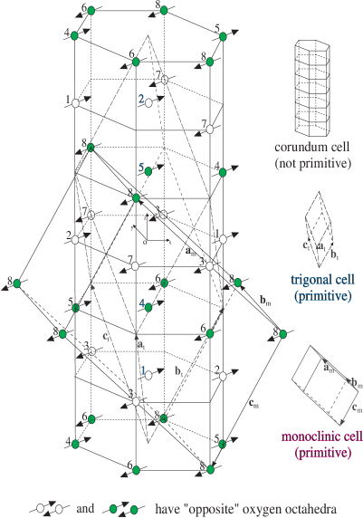
Figure 1 shows the non primitive hexagonal unit cell of V₂O₃, together with the primitive trigonal one, in the corundum paramagnetic phase. Only Vanadium atoms are shown. There are two formula units per cell (four V atoms) and each metal ion is surrounded by a slightly distorted oxygen octahedron with the three-fold symmetry axis directed along the c_H-hexagonal vertical axis. The distortion corresponds to a compression of the octahedron along c_H. The octahedra around the V-ions represented by the filled circles in Fig. 1 are rotated by $180^{o}$ about the c_H axis with respect to those around the V-ions represented by the empty circles, this orientation varying from plane to plane. Only 2/3 of the octahedra centers are occupied by the metallic ion. The space group of the corundum phase is $R\overline{3}c$ with the following generators (written in the conventional notation[30]):

$$\begin{array}[]{lll}\{{\hat{E},0}\}&=&{\rm Identity}\\ \{{\hat{I},0}\}&=&{\rm Inversion~{}around~{}the~{}midpoint~{}of~{}V_{4}}\\ &&{\rm and~{}V_{5}~{}(point~{}O~{}in~{}Fig.~{}\ref{boh})}\\ \{{\hat{C}_{3},0}\}&=&{\rm Rotation~{}of~{}}\pi/3{\rm~{}around~{}the~{}c_{H}~{}axis}\\ \{{\hat{C}_{2},\frac{1}{2}\vec{a}_{m}}\}&=&{\rm Rotation~{}of~{}}\pi{\rm~{}around~{}the~{}}\vec{b}_{m}{\rm~{}axis}\\ &&{\rm followed~{}by~{}a~{}translation~{}of~{}\frac{1}{2}}\vec{a}_{m}~{},\\ \end{array}$$ (88)

where $\vec{a}_{m}$ and $\vec{b}_{m}$ are two of the basis vectors of the monoclinic unit cell shown in Fig. 1. The origin O has been chosen as the inversion point between atom V₄ and V₅ in the trigonal cell. The translation associated with the $\hat{C}_{2}$ rotation can be expressed also in terms of the trigonal basis vectors defined in Fig. 1 as $\frac{1}{2}(\vec{a}_{t}+\vec{b}_{t}+\vec{c}_{t})$. The corresponding crystal point group, obtained by setting all translations to zero, is $D_{3d}$.[30] Note that among the symmetry operations of $R\overline{3}c$ there is a glide plane, obtained through the combination of $\hat{I}$ and $\hat{C}_{2}$:

$$\begin{array}[]{lll}\{\hat{\sigma}_{b},\frac{1}{2}\vec{a}_{m}\}&=&{\rm Reflection~{}through~{}a~{}plane~{}orthogonal}\\ &&{\rm to~{}the~{}}\vec{b}_{m}{\rm~{}axis~{}followed~{}by~{}a~{}translation}\\ &&{\rm of~{}\frac{1}{2}}\vec{a}_{m}~{}.\\ \end{array}$$ (92)

By lowering the temperature, the system makes a disruptive first order transition to a monoclinic phase, with further distortion of the octahedra to accommodate a rotation by about $1.8^{o}$ of the vertical Vanadium pairs (e.g., V₁ and V₄) in the $a_{m}-c_{m}$ plane towards the adjacent octahedral voids.[3] As a consequence one bond in the basal plane becomes longer than the other two by about 0.1 Å, the trigonal symmetry is lost and the lattice space group lowers to $I2/a$ with the same generators except for $(\hat{C}_{3},0)$. Its crystal point group is $C_{2h}$. The monoclinic cell is body-centered and, containing four formula units, it is not primitive, from the point of view of the bare crystal lattice. However concomitant to the structural transition a magnetic order sets in, with ferromagnetic $a_{m}-c_{m}$ planes stacked antiferromagnetically and with an AF wave vector given by $\frac{1}{2}\vec{b}_{m}$.[4] Because of this magnetic order, the monoclinic cell becomes primitive, due to the AF coupling of the magnetic moments on the V-ions connected by the body-centered translation. The magnetic moments of the V-ions, indicated by arrows in the figure, lie in the $a_{m}-c_{m}$ plane, at an angle of $71^{o}$ away from the c_H axis.[4, 6] Notice that the in-plane longer bond corresponds to the ferromagnetic coupling and is orthogonal to $\vec{b}_{m}$.

Under these conditions one can easily check that the time-reversal operator $\hat{T}$ followed by the non primitive translation $\frac{1}{2}(\vec{a}_{m}+\vec{b}_{m}+\vec{c}_{m})$ is a symmetry operation of the magnetic structure, so that the magnetic point group is $C_{2h}\otimes\hat{T}$. Each operation should be followed by the appropriate translation as indicated here:

$$\begin{array}[]{lll}1){\rm~{}}{\hat{E}},{\rm~{}}{\hat{I}}&\rightarrow&{\rm No~{}translations}\\ 2){\rm~{}}{\hat{C}_{2}},{\rm~{}}{\hat{\sigma}_{b}}&\rightarrow&\frac{1}{2}(\vec{b}_{m}+\vec{c}_{m})\\ 3){\rm~{}}{\hat{T}},{\rm~{}}{\hat{T}\hat{I}}&\rightarrow&\frac{1}{2}(\vec{a}_{m}+\vec{b}_{m}+\vec{c}_{m})\\ 4){\rm~{}}{\hat{T}\hat{C}_{2}},{\rm~{}}{\hat{T}\hat{\sigma}_{b}}&\rightarrow&\frac{1}{2}\vec{a}_{m}~{}.\end{array}$$ (97)

Notice that the translation associated to $\hat{C}_{2}$ and $\hat{\sigma}_{b}$ has changed. In fact, since now the application of these two operations changes the direction of the magnetic moment,[30] the total translation must be

$$\frac{1}{2}\vec{a}_{m}+\frac{1}{2}(\vec{a}_{m}+\vec{b}_{m}+\vec{c}_{m})\equiv\frac{1}{2}(\vec{b}_{m}+\vec{c}_{m})$$

and the role of $\hat{C}_{2}$ and $\hat{\sigma}_{b}$ in the paramagnetic lattice is taken, in the AFI phase, by $\hat{T}\hat{C}_{2}$ and $\hat{T}\hat{\sigma}_{b}$.

Under these operations the correspondence between the charge and magnetic states of the various metal sites with their oxygen environment is given in Table I, with reference to the numbering of Fig. 1:

Table I. Correspondence table between magnetic sites in V₂O₃

$\begin{array}[]{||l|c|c|c|c|c|c|c|c||}\hline\cr\hat{E}:&1&2&3&4&5&6&7&8\\ \hline\cr\hat{I}:&2&1&7&5&4&8&3&6\\ \hline\cr\hat{C}_{2}:&8&6&5&7&3&2&4&1\\ \hline\cr\hat{\sigma}_{b}:&6&8&4&3&7&1&5&2\\ \hline\cr\hat{T}:&7&3&2&8&6&5&1&4\\ \hline\cr\hat{T}\hat{I}:&3&7&1&6&8&4&2&5\\ \hline\cr\hat{T}\hat{C}_{2}:&4&5&6&1&2&3&8&7\\ \hline\cr\hat{T}\hat{\sigma}_{b}:&5&4&8&2&1&7&6&3\\ \hline\cr\end{array}$

Now the recent observation of non reciprocal x-ray gyrotropy by Goulon et al. [21] in the AFI phase of V₂O₃ points to a reduction of magnetic symmetry. In this experiment a transverse x-ray linear dichroism at the Vanadium K-edge is observed and interpreted as due to a dipole-quadrupole interference effect. This signal changes sign according to whether the externally applied magnetic field is parallel or antiparallel to the direction of the incident x-ray beam along the $c_{H}$ axis. Therefore neither $\hat{T}$ nor $\hat{I}$ can be separately symmetry operations, but their product $\hat{T}\hat{I}$ is. There are seven subgroups of four elements of the magnetic point group $C_{2h}\otimes\hat{T}$. They are listed below:

$$1.~{}~{}~{}~{}~{} \hat{E},\hat{I},\hat{C}_{2},\hat{\sigma}_{b}$$

$$2.~{}~{}~{}~{}~{} \hat{E},\hat{I},\hat{T},\hat{T}\hat{I}$$

$$3.~{}~{}~{}~{}~{} \hat{E},\hat{I},\hat{T}\hat{C}_{2},\hat{T}\hat{\sigma}_{b}$$

$$4.~{}~{}~{}~{}~{} \hat{E},\hat{T},\hat{C}_{2},\hat{T}\hat{C}_{2}$$

$$5.~{}~{}~{}~{}~{} \hat{E},\hat{T},\hat{\sigma}_{b},\hat{T}\hat{\sigma}_{b}$$

$$6.~{}~{}~{}~{}~{} \hat{E},\hat{C}_{2},\hat{T}\hat{I},\hat{T}\hat{\sigma}_{b}$$

$$7.~{}~{}~{}~{}~{} \hat{E},\hat{\sigma}_{b},\hat{T}\hat{I},\hat{T}\hat{C}_{2}~{}.$$

It is immediately clear that only groups 6 and 7 are eligible candidates, i.e., group $C_{2h}(C_{s})$ and $C_{2h}(C_{2})$, respectively $\underline{2}/m$ and $2/\underline{m}$ in international notation. Both are magnetoelectric (ME); however the first one gives rise to an off-diagonal ME tensor whereas in the second one this tensor presents diagonal components. [31] It is possible to discriminate between them by noting that the existence of an off-diagonal ME tensor explains why Astrov and Al'shin failed[32] to find a ME effect in V₂O₃, since their experiment was set up to look for diagonal components. This is a strong indication that $C_{2h}(C_{s})$ is the correct magnetic group for V₂O₃.

The origin of the reduction of magnetic symmetry from $C_{2h}\otimes\hat{T}$ to $C_{2h}(C_{s})$ can reasonably be ascribed to an orbital ordering in the magnetic and charge density of V₂O₃ due to electron correlations. However the ferro-orbital C phase found by Mila et al.[19] does not provide the correct answer, since the corresponding magnetic group is easily seen to be $C_{2h}\otimes\hat{T}$, due to the fact that all sites are occupied by the same orbital. The same can be said for the other stable phases with the real spin structure found in this work.

We speculate that the presence of an excited configuration with the correct magnetic group $C_{2h}(C_{s})$, very near the ground state and with the favorable coupling with the lattice, can provide the solution to this puzzle.

FIG. 2.: The neighbor structure of the vertical bonds. Referring to Fig.1, if the atom $a$ coincides with V₁, then we have the correspondences $b\rightarrow$ V₄, $c\rightarrow$ V₂, $c^{\prime}\rightarrow$ V₅, $d\equiv e\rightarrow$ V₃, and $d^{\prime}\equiv e^{\prime}\rightarrow$ V₆.

In order to proceed in the following sections with the minimization of $H_{\rm eff}$ we need to have a reasonable guess at the various parameters appearing in it, namely the hopping integrals and the Coulomb and exchange atomic parameters. In Fig. 2 we show half of the cluster of nearest neighbors to a given molecule (the other half can be deduced with the help of Fig. 1) to illustrate the notation that will be used later on.

Following CNR[7, 8] we present in Table II the transfer integrals evaluated by exploiting the symmetry properties of the corundum structure without taking into account the monoclinic distortion of the bonds, since again our aim is to show how electronic correlations can break the initial trigonal symmetry of the lattice. The deviations from this symmetry will be considered later on to illustrate if and how the monoclinic distortion can stabilize the orbitally ordered state with the correct magnetic spin structure.

Table II. Transfer integrals along different bonds in the corundum phase.

direction	$\delta_{1}$	$\delta_{2}$	$\delta_{3}$	$\delta_{4}$
$t_{11}$	$-\alpha$	$-\frac{1}{4}\alpha+\frac{3}{4}\beta$	$-\frac{1}{4}\alpha+\frac{3}{4}\beta$	$\mu$
$t_{22}$	$\beta$	$-\frac{3}{4}\alpha+\frac{1}{4}\beta$	$-\frac{3}{4}\alpha+\frac{1}{4}\beta$	$\mu$
$t_{33}$	$\sigma$	$\sigma$	$\sigma$	$\rho$
$t_{12}$	0	$\frac{\sqrt{3}}{4}(\alpha+\beta)$	$-\frac{\sqrt{3}}{4}(\alpha+\beta)$	0
$t_{13}$	0	$\frac{\sqrt{3}}{2}\tau$	$-\frac{\sqrt{3}}{2}\tau$	0
$t_{23}$	$-\tau$	$\frac{1}{2}\tau$	$\frac{1}{2}\tau$	0
$t_{21}$	0	$\frac{\sqrt{3}}{4}(\alpha+\beta)$	$-\frac{\sqrt{3}}{4}(\alpha+\beta)$	0
$t_{31}$	0	$\frac{\sqrt{3}}{2}\tau$	$-\frac{\sqrt{3}}{2}\tau$	0
$t_{32}$	$-\tau$	$\frac{1}{2}\tau$	$\frac{1}{2}\tau$	0

Table III. Transfer integrals (eV) from tight binding calculations used by CNR[8] and from LAPW-calculations by Mattheiss.[33]

	Castellani et al.[8]	Mattheiss[33]
$\mu$	$0.2$	$0.2$
$\rho$	$-0.72$	$-0.82$
$-\alpha$	$-0.13$	$-0.14$
$\beta$	$-0.04$	$-0.05$
$\sigma$	$0.05$	$0.05$
$-\tau$	$-0.23$	$-0.27$

In the following we shall assume for the Coulomb and exchange parameters the values suggested by Ezhov et al.[16] and Mila et al.[19] i.e., $J\simeq 0.7\div 1.0~{}eV$, $U_{2}\sim 2.5~{}eV$, and for the hopping parameters those derived by Mattheiss[33] and shown in Table III. This set will be referred as the standard set. By fitting the LAPW band structure of V₂O₃ to a tight-band calculation, Mattheiss [33] has provided the relevant Slater-Koster integrals that have been used to calculate the appropriate hopping integrals. As on can see from Table III they are quite close to those estimated by CNR. [7, 8]

V The energetics of the vertical molecule.

As realized by CNR [7, 8] and later by Mila et al., [19] the formation of the vertical molecular bond ($\delta_{4}$ in Fig. 2) is the key to the understanding of the physics of V₂O₃ in all three phases. This fact is indeed supported by the experimental evidence both from optical spectra [20] and inelastic neutron scattering.[6, 10] However the solution proposed by CNR was appropriate to low values of $J$ ($\leq$ 0.2 eV) and values of the trigonal distortion which where supposed to be quite small, as suggested by Rubinstein. [34] The new solution proposed by Mila et al. [19] reconciles the present evidence for an high value of $J$ ($\geq$ 0.7 eV) and the consequent spin $S=1$ state of the V-ions [13, 14] with the existence of an orbitally degenerate molecular state, while being rather stable against a sizable value of the trigonal distortion. It is interesting to study how this can come about, since this investigation can provide a clue to the kind of variational wave function to be used in the minimization of $H_{\rm eff}$, will delimit the regions of stability of the solution in the parameter space and indicate competing states that might be relevant for the phenomenon of the metal-insulator transition in V₂O₃.

A The approximate solution using $H_{\rm eff}$

In considering the vertical pair it is convenient, as shown in Section V-B, to introduce the following molecular quantum numbers: the total spin $S^{M}=S_{a}+S_{b}$, its $z$-component $S^{M}_{z}=S_{az}+S_{bz}$ and total $z$-component of pseudospin $\tau_{z}^{M}=\tau_{az}+\tau_{bz}$. Along the vertical bond $\delta_{4}$ only $t_{11}=t_{22}=\mu$ and $t_{33}=\rho$ are different from zero (as seen from Table II) and their values are given in Table III. Specializing to this case the effective Hamiltonian given in Appendix C we obtain for the ferromagnetic state ($S^{M}=2$) the following expression:

$$H_{\rm eff}^{F} = -\frac{1}{3}\frac{1}{U_{2}-J}{\big{[}}2+\vec{S}_{a}\cdot\vec{S}_{b}{\big{]}}(\mu^{2}f_{\mu}+\rho^{2}f_{\rho}-\mu\rho f_{\mu\rho})~{},$$ (98)

and for the antiferromagnetic bond ($S_{M}=0$):

$$H_{\rm eff}^{A} = -\frac{1}{2}\frac{1}{U_{2}+4J}{\big{[}}1-\vec{S}_{a}\cdot\vec{S}_{b}{\big{]}}$$ (105)

$$\times[\mu^{2}(a_{\mu}+a^{\prime}_{\mu})+\rho^{2}a_{\rho}+\frac{1}{2}\mu\rho a_{\mu\rho}]$$

$$-\frac{1}{2}\frac{1}{U_{2}+2J}{\big{[}}1-\vec{S}_{a}\cdot\vec{S}_{b}{\big{]}}$$

$$\times[\mu^{2}(a_{\mu}-a^{\prime}_{\mu})+\rho^{2}a_{\rho}-\frac{1}{2}\mu\rho a_{\mu\rho}]$$

$$-\frac{1}{6}\frac{1}{U_{2}+2J}{\big{[}}1-\vec{S}_{a}\cdot\vec{S}_{b}{\big{]}}$$

$$\times[2\mu^{2}a^{\prime\prime}_{\mu}+2\rho^{2}a^{\prime\prime}_{\rho}+\mu\rho a^{\prime\prime}_{\mu\rho}]~{},$$

where, respectively, we have defined:

$$f_{\mu} = \tau_{az}^{2}+\tau_{bz}^{2}-\tau_{az}\tau_{bz}-\tau_{az}^{2}\tau_{bz}^{2}$$ (107)

$$-\frac{1}{2}\tau_{a}^{-}\tau_{a}^{-}\tau_{b}^{+}\tau_{b}^{+}-\frac{1}{2}\tau_{a}^{+}\tau_{a}^{+}\tau_{b}^{-}\tau_{b}^{-}$$

$$f_{\rho} = \tau_{az}^{2}+\tau_{bz}^{2}-2\tau_{az}^{2}\tau_{bz}^{2}$$ (108)

$$f_{\mu\rho} = \tau_{a}^{-}\tau_{az}\tau_{bz}\tau_{b}^{+}+\tau_{az}\tau_{a}^{-}\tau_{b}^{+}\tau_{bz}$$ (110)

$$+\tau_{a}^{+}\tau_{az}\tau_{bz}\tau_{b}^{-}+\tau_{az}\tau_{a}^{+}\tau_{b}^{-}\tau_{bz}$$

and

$$a_{\mu} = 2-\tau_{az}^{2}-\tau_{bz}^{2}+\frac{1}{2}(\tau_{az}\tau_{bz}+\tau_{az}^{2}\tau_{bz}^{2})$$ (111)

$$a^{\prime}_{\mu} = +\frac{1}{4}(\tau_{a}^{-}\tau_{a}^{-}\tau_{b}^{-}\tau_{b}^{-}+\tau_{a}^{+}\tau_{a}^{+}\tau_{b}^{+}\tau_{b}^{+})$$ (112)

$$a_{\mu\rho} = \tau_{a}^{-}\tau_{az}\tau_{b}^{-}\tau_{bz}+\tau_{az}\tau_{a}^{-}\tau_{bz}\tau_{b}^{-}$$ (114)

$$+\tau_{a}^{+}\tau_{az}\tau_{b}^{+}\tau_{bz}+\tau_{az}\tau_{a}^{+}\tau_{bz}\tau_{b}^{+}$$

$$a_{\rho} = \tau_{az}^{2}\tau_{bz}^{2}$$ (115)

$$a^{\prime\prime}_{\mu} = \tau_{az}^{2}+\tau_{bz}^{2}-\tau_{az}\tau_{bz}-\tau_{az}^{2}\tau_{bz}^{2}$$ (117)

$$+\frac{1}{4}(\tau_{a}^{-}\tau_{a}^{-}\tau_{b}^{+}\tau_{b}^{+}+\tau_{a}^{+}\tau_{a}^{+}\tau_{b}^{-}\tau_{b}^{-})$$

$$a^{\prime\prime}_{\rho} = \tau_{az}^{2}+\tau_{bz}^{2}-2\tau_{az}^{2}\tau_{bz}^{2}$$ (118)

$$a^{\prime\prime}_{\mu\rho} = \tau_{a}^{-}\tau_{az}\tau_{bz}\tau_{b}^{+}+\tau_{az}\tau_{a}^{-}\tau_{b}^{+}\tau_{bz}$$ (120)

$$+\tau_{a}^{+}\tau_{az}\tau_{bz}\tau_{b}^{-}+\tau_{az}\tau_{a}^{+}\tau_{b}^{-}\tau_{bz}~{}.$$

We assume for the moment $\Delta_{t}=0$. Based on Eq. (LABEL:fb) and with the definitions of Eq. (107) we can easily evaluate eigenvalues and eigenstates of $H_{\rm eff}^{F}$. Neglecting the 5-fold spin degeneracy and taking into account only the orbital one, we find the following doubly degenerate ground state with $\tau^{M}_{z}=\pm 1$:

$$|\psi^{o}_{\pm}\rangle_{ab}=\frac{1}{\sqrt{2}}(|\pm 1\rangle_{a}|0\rangle_{b}+|\pm 1\rangle_{b}|0\rangle_{a})$$ (121)

Equation (121) represents only the orbital part of the ground state. The whole state (e.g., with $S^{M}_{z}=2$) can be pictured as:

or as

The corresponding ground state energy is:

$$\Delta E_{m}=-\frac{(\mu-\rho)^{2}}{U_{2}-J}~{}.$$ (122)

With reference to the picture of the state, this energy lowering (with respect to the atomic limit $2(U_{2}-J)$) is made up of three terms: the virtual hopping back and forth of an $e_{g}$ electron ($-\frac{\mu^{2}}{U_{2}-J}$), the similar process for the $a_{1g}$ electron ($-\frac{\rho^{2}}{U_{2}-J}$) and a sort of correlated hopping in which an $e_{g}$ electron jumps from atom $a$ to atom $b$ while simultaneously an $a_{1g}$ electron jumps from atom $b$ to atom $a$ and vice-versa ($\frac{2\rho\mu}{U_{2}-J}$, which is negative due to the opposite sign of $\rho$ and $\mu$, see Table III). This latter process is present only due to the ``entangled'' orbital nature of the molecular state of Eq. (121) and is absent in its Hartree-Fock approximation, which provides a lowering of only $\Delta E_{HF}=-\frac{\mu^{2}+\rho^{2}}{U_{2}-J}$. With the values given in Table III, the ratio between the interference and the HF term $2\mu\rho/(\mu^{2}+\rho^{2})$ is of the order of 50%. Therefore the molecular correlation energy $\Delta E_{m}-\Delta E_{HF}=\frac{2\mu\rho}{U_{2}-J}$ is much bigger than the in-plane exchange energy ($\approx\frac{\alpha^{2}+\tau^{2}}{U_{2}-J}$), so that in this case the best variational wave function for the entire crystal should be constructed in terms of molecular states.

Another point worth mentioning here is the quality of the expansion around the atomic limit. The exact solution of the $2\times 2$ eigenvalue problem for the ferromagnetic vertical molecule is given by

$$\Delta E_{m} = E_{m}-2(U_{2}-J)$$ (123)

$$= \frac{(U_{2}-J)}{2}\left(1-\sqrt{1+\frac{4(\mu-\rho)^{2}}{(U_{2}-J)^{2}}}\right)~{}.$$ (124)

We see from this expression that the expansion parameter is $\frac{2(\mu-\rho)}{(U_{2}-J)}$, which is of the order of one, using the standard values of Table III. This value is borderline for a good expansion; however, as often happens in perturbation theory, the second order term turns out to be a reasonable approximation to the exact result ($1+0.89$ as compared to $\sqrt{2.78}=1.67$, with a relative error of less than $13\%$ in the worst of the cases). Moreover this problem is present only for the vertical pairs, since in the basal plane we are well within the values for a rapidly convergent expansion. Notice that, when comparing different variational minimal solutions of $H_{\rm eff}$ in section VI, the error in the vertical pairs will cancel out and the result will be of the same accuracy as the expansion for bonds in the basal plane.

As long as $|\rho|\!\!>\!\!|\mu|$, the ferromagnetic state with $S^{M}=2$ in Eq. (121) is the ground state for the vertical pair. However it is easy to realize that, in the opposite case $|\rho|<|\mu|$, the orbital part of the ground state changes to

$$|\psi^{o}_{0}\rangle_{ab}=\frac{1}{\sqrt{2}}(|1\rangle_{a}|-1\rangle_{b}+|1\rangle_{b}|-1\rangle_{a})$$ (125)

or, pictorially, including the spin ($S^{M}_{z}=2$):

with an energy lowering of $\Delta E_{m}^{\prime}=-\frac{4\mu^{2}}{U_{2}-J}$.

This state is not orbitally degenerate. However it is interesting to note that in this case the percentage of occupation of the $a_{1g}$ state is 50%, so that this solution is excluded by the findings of Park et al.,[14] as well as on the basis of the theoretical estimates of Table III ($\rho\!>\!\mu$).

As long as $\frac{J}{U_{2}}>0.22$ the ferromagnetic configuration in Eq. (121) remains the ground state of the pair. By decreasing $J$ a transition to an antiferromagnetic ($S^{M}=0$) ground state is expected, since this spin configuration will maximize the number of virtual hopping processes without loosing too much in Hund's energy. This is indeed what happens when $\frac{J}{U_{2}}<0.22$.

Even in this case we obtain a two-fold orbitally degenerate ground state:

$$|\psi^{o}_{|2|}\rangle_{ab}\simeq\frac{1}{\sqrt{2}}(|-1\rangle_{a}|-1\rangle_{b}-|1\rangle_{b}|1\rangle_{a})~{},$$ (126)

and

$$|\psi^{o}_{0}\rangle_{ab}\simeq\frac{1}{\sqrt{2}}(|-1\rangle_{a}|1\rangle_{b}+|-1\rangle_{b}|1\rangle_{a})~{},$$ (127)

For simplicity of presentation we have omitted to show the spin structure of this state, since this latter is given in the following section V-B (see states $|\gamma_{1}\rangle$ and $|\gamma_{2}\rangle$ of Eq. (136)). The ground state energy is given by:

$$\Delta E^{AF}_{m}=-\frac{3}{2}\bigg{[}\frac{\rho^{2}}{U_{2}+4J}+\frac{\rho^{2}+2\mu^{2}}{U_{2}+2J}\bigg{]}~{}.$$ (128)

Note that the first state (Eq. (126)), mixing the values $\tau_{z}^{M}=\pm 2$ does not conserve the value of pseudospin $z$-component, due to the term $H_{0j}^{(4)}$ in Eq. (15).

The above level scheme is confirmed by the exact treatment of the vertical pair on the basis of the original Hubbard Hamiltonian which is reported in the following section V-B. There are slight discrepancies, however, due to the non optimal conditions for perturbation theory. For example, the transition value between the ferromagnetic and antiferromagnetic configurations is found at $\frac{J}{U_{2}}=0.29$. Moreover the degeneracy of the two antiferromagnetic states is removed, the second lying always lowest (from 1 to 5 meV, in the range of parameters of interest), due to the different mixing with states that have been projected out in the perturbation theory (those with $S_{a}=S_{b}=0$ and those with $S_{a}=S_{b}=1/2$). In general, though, the exact energy level structure is reasonably close to the approximate one.

By switching on the trigonal distortion $\Delta_{t}$, the ferromagnetic ground state energy (122) changes to

$$\Delta E_{mt}=-\frac{(\mu-\rho)^{2}}{U_{2}-J}+\Delta_{t}$$ (129)

and the antiferromagnetic (128) becomes

$$\Delta E^{AF}_{mt1}=-\frac{3}{2}\bigg{[}\frac{\rho^{2}}{U_{2}+4J}+\frac{\rho^{2}+2\mu^{2}}{U_{2}+2J}\bigg{]}+2\Delta_{t}~{}.$$ (130)

Because of this, the stability region of the ferromagnetic state in the parameter $\frac{J}{U_{2}}$ initially increases with $\Delta_{t}$, since its $a_{1g}$ population is only 25%, compared to the 50% value of the antiferromagnetic states. However for $\Delta_{t}$ bigger than a critical value $\overline{\Delta}_{t}$ there is an inversion of tendency and the stability region begins to decrease. This is due to the fact that the structure of the antiferromagnetic state changes abruptly from a situation in which the $a_{1g}$ population is 50% to one in which is 0%. Indeed for $\Delta_{t}\geq\overline{\Delta}_{t}$ the lowest energy configuration for the AF bond is reached when the two electrons on each site occupy both $e_{g}$ orbitals and are coupled to spin $S=1$, with total spin $S^{M}=0$: in this case the ground state orbital configuration, for $J$ not too close to zero (i.e., $J\geq 0.2$ eV, due to the constraint $2J\geq\Delta_{t}$ used in our perturbation theory) is given by:

(131)

The full spin structure of the state (131) will be given in the next subsection (see state $|\gamma_{9}\rangle$). The ground state AF energy, in this case, is:

$$\Delta E^{AF}_{mt2}=-3\mu^{2}\bigg{[}\frac{1}{U_{2}+4J}+\frac{1}{U_{2}+2J}\bigg{]}~{}.$$ (132)

Finally the estimate of $\overline{\Delta}_{t}$, obtained by comparing Eqs. (129), (130) and (132), and using Mattheiss parameters of Table III, is $\overline{\Delta}_{t}\simeq 0.34~{}eV$, in good agreement with the exact value calculated in section V-B ($\overline{\Delta}_{t}\simeq 0.30~{}eV$).

We shall not dwell anymore on this subject since it will be studied more in depth in section V-B.

B The exact solution using the Hubbard Hamiltonian.

In constructing the effective Hamiltonian (see section II) we have assumed that $J$ is a high energy parameter and therefore have excluded from our zeroth order degenerate manifold singlet spin states, lying at higher energies by $2J$ or more. In order to assess the range validity of $H_{\rm eff}$ as a function of $J$ and the stability of the vertical molecule for $J\rightarrow 0$, we examine here the ground state configuration of the vertical molecule using Hubbard Hamiltonian ($H_{0}+H^{\prime}$). In this case the Hilbert space is made up of 495 atomic states with up to four electrons per site and the eigen-problem is rather complicated. However, due to the SU(2) invariance of the Hubbard Hamiltonian, states with different spin $S^{M}$ and different $S_{z}^{M}$ do not mix. Furthermore, since by assumption only diagonal hopping integrals are different from zero, the kinetic and crystal field terms $H^{\prime}$ in Eq. (17) do not change the total molecular pseudospin $\tau_{z}^{M}$, while the atomic part $H_{0}$ can only mix states with the same parity of $\tau_{z}^{M}$, due to the $H_{0j}^{(4)}$ term in Eq. (15). We can therefore divide the states of our Hilbert space into 6 groups which are characterized by the following quantum numbers:

1) $S^{M}=S_{z}^{M}=0$ and $\tau_{z}^{M}$ even (57 states):
    $\tau_{z}^{M}=\pm 4$ (2 states);
    $\tau_{z}^{M}=\pm 2$ (28 states);
    $\tau_{z}^{M}=0$ (27 states);
2) $S^{M}=S_{z}^{M}=0$ and $\tau_{z}^{M}$ odd (48 states):
    $\tau_{z}^{M}=\pm 3$ (8 states);
    $\tau_{z}^{M}=\pm 1$ (40 states);
3) $S^{M}=1$, $S_{z}^{M}$ fixed and $\tau_{z}^{M}$ even (49 states):
    $\tau_{z}^{M}=\pm 2$ (22 states);
    $\tau_{z}^{M}=0$ (27 states);
4) $S^{M}=1$, $S_{z}^{M}$ fixed and $\tau_{z}^{M}$ odd (56 states):
    $\tau_{z}^{M}=\pm 3$ (8 states);
    $\tau_{z}^{M}=\pm 1$ (48 states);
5) $S^{M}=2$, $S_{z}^{M}$ fixed and $\tau_{z}^{M}$ even (7 states):
    $\tau_{z}^{M}=\pm 2$ (2 states);
    $\tau_{z}^{M}=0$ (5 states);
6) $S^{M}=2$, $S_{z}^{M}$ fixed and $\tau_{z}^{M}$ odd (8 states):
    $\tau_{z}^{M}=\pm 1$ (8 states).

FIG. 3.: Energy eigenvalues of the Hubbard Hamiltonian for the vertical molecule as a function of $J$: solid line – $S^{M}=2$ and $\tau_{z}^{M}$ odd; dot-dot-dashed line – $S^{M}=1$ and $\tau_{z}^{M}$ even; dashed line – $S^{M}=0$ and $\tau_{z}^{M}$ even. Panels $(a),(b),(c)$ and $(d)$ correspond to the trigonal distortion $\Delta_{t}=0$ eV, $\Delta_{t}=0.1$ eV, $\Delta_{t}=0.3$ eV and $\Delta_{t}=0.4$ eV, respectively.

This classifications is valid for each $S_{z}^{M}$ component, so that for $S^{M}=1$ we get $(49+56)\times 3=315$ states and for $S^{M}=2$ we get $(7+8)\times 5=75$ states. It is worth noticing that when the $H_{0j}^{(4)}$ term in Eq. (15) is not effective, $\tau_{z}^{M}$ is conserved and further reduction of the number of mixing states is possible. This is the case for all the states with $S^{M}=2$, where the 15 states of fixed $S_{z}^{M}$ component can be grouped into the orthogonal sets: $\tau_{z}^{M}=+2$ (1 state), $\tau_{z}^{M}=+1$ (4 states), $\tau_{z}^{M}=0$ (5 states), $\tau_{z}^{M}=-1$ (4 states), $\tau_{z}^{M}=-2$ (1 state).

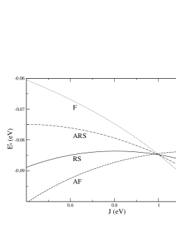
We take the standard values of the parameters (Mattheiss set) and look at the eigenvalue structure as a function of $J$ for different subgroups of the Hilbert space (see Fig. 3). For this choice of the parameters the three lowest energies are always in the groups of states with $S^{M}=0$ and $\tau_{z}^{M}$ even, $S^{M}=1$ and $\tau_{z}^{M}$ even or $S^{M}=2$ and $\tau_{z}^{M}$ odd. They are presented in Fig. 3.

The crystal field degenerate case ($\Delta_{t}=0$ eV) is presented in the Fig. 3$(a)$. For $J\rightarrow 0$ eV the ground state of the vertical pair belongs to the sector $S^{M}=0$ with $\tau_{z}^{M}$ even. By increasing $J$ three transitions occur. At very low $J\sim 0.04$ eV a first transition to a state with $S^{M}=1$ with $\tau_{z}^{M}$ even takes place. This state is reminiscent of the ground state postulated by CNR [7] for the vertical molecule (about $55\%$ of its weight is composed by the old CNR state for $J=0.04$) and, because of this, it does not belong to the Hilbert subspace upon which $H_{\rm eff}$ can operate. In this region the $S^{M}=0$ with $\tau_{z}^{M}$ even state lies only 3 meV higher in energy. Then at $J\simeq 0.17$ eV a second transition takes place again toward a state with $S^{M}=0$ and $\tau_{z}^{M}$ even. To get an idea of its composition in terms of atomic states, we give its expression at $J=0.73$ eV, that is the upper boundary of the region of stability of the $S^{M}=0$ state. Note, that even though the weight of the particular state depends on the value of $J$, the tendency of the weight distribution is the same in the whole region $0.17$ eV$\leq J\leq 0.73$ eV. We get:

$$\begin{array}[]{l}\parallel GS\rangle_{J=0.73}\simeq 0.67|\gamma_{1}\rangle+0.67|\gamma_{2}\rangle\\[8.5359pt] +0.14|\gamma_{3}\rangle+0.14|\gamma_{4}\rangle+0.14|\gamma_{5}\rangle+0.14|\gamma_{6}\rangle~{},\end{array}$$ (135)

where

This state is essentially composed by

$$\parallel GS\rangle_{J=0.73}\simeq\frac{1}{\sqrt{2}}(|\gamma_{1}\rangle+|\gamma_{2}\rangle)$$ (136)

i.e., the $\tau^{M}_{z}=0$ combination of nonpolar atomic spin-1 states coupled to $S^{M}=0$. Its orbital part is the same as the state $|\psi^{o}_{0}\rangle_{ab}$ mentioned in Eq. (127), of which it is the complete spin orbital representation. Note that the same spin structure belongs also to the state $|\psi^{o}_{|2|}\rangle_{ab}$ given by Eq. (126), even if the orbital part is different.

At still greater $J$, the value $J\sim 0.73$ marks the final transition to the doubly degenerate ferromagnetic state with $S^{M}=2$ and $\tau_{z}^{M}=\pm 1$, which is therefore stable for $J/U_{2}\geq 0.29$. We have two $2\times 2$ eigenvalue equations for both $\tau_{z}^{M}=\pm 1$. Choosing $\tau_{z}^{M}=-1$ and solving for the ground state, we get:

$$\parallel GS\rangle_{J\geq 0.73}=N\left(~{}|\gamma_{7}\rangle+C~{}|\gamma_{8}\rangle~{}\right)$$ (137)

where $C=\frac{U_{2}-J}{2(\mu-\rho)}\left(1-\sqrt{1+\frac{4(\mu-\rho)^{2}}{(U_{2}-J)^{2}}}\right)$, $N$ is an appropriate normalization factor and, for $S^{M}_{z}=2$,

Notice that the state in Eq. (121) is nothing else that the atomic limit of $|GS\rangle_{J\geq 0.73}$ (actually, $|\gamma_{7}\rangle\equiv|\gamma_{-}\rangle_{ab}$). For the chosen values of the parameters and $J=0.73$ eV the component $|\gamma_{7}\rangle$ represents 83% of the total weight and increases with increasing $J$.

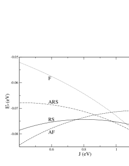
To demonstrate the role of the trigonal distortion $\Delta_{t}$ on the stability region of the various ground states, we consider different values up to 0.4 eV, which is the value suggested by Ezhov et al. [16] As seen from Fig. 3$(a)$ to Fig. 3$(c)$, for values of $\Delta_{t}$ up to 0.3 eV the role of the trigonal splitting is essentially to decrease the value of $J$ at which the $S^{M}=0\rightarrow S^{M}=2$ transition takes place, i.e., to increase the stability region of the ferromagnetic state. As already anticipated in the previous subsection, this fact can be easily explained by looking at the structure of the $S^{M}=2$ state, essentially composed by $|\gamma_{7}\rangle$ with 25% of $a_{1g}$ occupancy, and the $S^{M}=0$ state, given in Eq. (136) and composed by $|\gamma_{1}\rangle$ and $|\gamma_{2}\rangle$, with 50% of $a_{1g}$ occupancy. At $\Delta_{t}\simeq 0.3$ eV an abrupt transition in the composition of the $S^{M}=0$ ground state takes place such that the preferred orbital occupation change to the $e_{g}$ states (no $a_{1g}$ orbitals, see state $|\gamma_{9}\rangle$), while the $S^{M}=2$ remains the same. As a consequence the stability region of this latter starts decreasing, as shown in Figs. 3$(c)$, $(d)$. This transition in the composition of the $S^{M}=0$ state had to be expected, since for $\frac{\Delta_{t}}{J},\frac{\Delta_{t}}{\rho}\rightarrow\infty$ the $a_{1g}$ occupation must go to zero.

FIG. 4.: Energy level structure at $J=1.0$ eV for molecular states with $S^{M}=2$, $\tau_{z}^{M}$ odd; $S^{M}=1$, $\tau_{z}^{M}$ even and $S^{M}=0$, $\tau_{z}^{M}$ even. Panels $(a),(b),(c)$ and $(d)$ correspond to the trigonal distortion $\Delta_{t}=0$ eV, $\Delta_{t}=0.1$ eV, $\Delta_{t}=0.3$ eV and $\Delta_{t}=0.4$ eV, respectively. Dot-dashed, dashed and solid lines indicate two, one or zero atomic $a_{1g}$ orbital occupancy in the ground state.

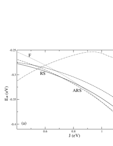
Figure 4$(a)$-$(d)$ illustrate how the low lying level structure and the composition of the ground state of the vertical pair changes as a function of $\Delta_{t}$. We fix $J=1.0~{}eV$, for reasons that will be apparent in the next section, although the same results are qualitatively valid for all the physical values of $J$. The main difference is that below the chosen value of $1.0$ eV, the energy gap between the $S^{M}=2$ ground state and the excited $S^{M}=0$ and $S^{M}=1$ states reduces, while above $J=1.0$ eV, it increases. At low values of $\Delta_{t}$ there are many low-lying excited levels for $S^{M}=0$, $\tau_{z}^{M}$ even states (dot-dashed lines of Fig.4$(a)$ and $(b)$). The orbital part of the two lowest states in this situation is given by Eqs. (126) and (127) and their energy difference is about $6$ meV. Notice that the lowest state is exactly given by Eq. (136). For the chosen value of $J=1.0$ eV, at $\Delta_{t}\sim 0.18$ eV there is a drastic redistribution of the weight in the atomic configuration of the $S^{M}=0$ molecule state, i.e., the non polar state is now given by

which is nothing else that the complete spin-orbit representation of the state (131). By further increasing $\Delta_{t}$ (see Fig. 3$(c)$ and $(d)$) this state becomes more and more favorable and finally at $\Delta_{t}\simeq 0.47$ becomes the overall ground state. At this value of $\Delta_{t}$ the weight of the non polar state $|\gamma_{9}\rangle$ is more than 99%. Note that the value of the crystal field splitting where we have the transition from a $S^{M}=2$ to a $S^{M}=0$ overall ground state does depend on $J$ as is clear from Figs. 3.

For $J=1.0$ eV the $S^{M}=1$, $\tau_{z}^{M}$ even state is never the ground state of the vertical molecule. Nevertheless at $\Delta_{t}=0.4$ eV (see Fig. 4$(d)$) it lies only about 80 meV above the ground state with $S^{M}=2$ and its composition is made up for more than 99% of the following state (e.g., with $S^{M}_{z}=1$):

As is clear from Fig. 3$(d)$, its excitation energy decreases with $J$. Note that $|\gamma_{10}\rangle$ is made up of two atomic $S=1$ states, so that it belongs to the subspace of $H_{\rm eff}$.

We shall make use of these findings later on in order to determine the various parameters in the AFI phase of V₂O₃.

VI The minimization procedure.

In this section we look for all the possible orbital and magnetic ground-state configurations of the effective Hamiltonian by using a variational procedure. The trial wave function can be written in general as follows:

$$|\Psi\rangle=\Pi_{n}~{}|\Psi_{n}\rangle=\Pi_{n}~{}|\psi^{o}_{n}\rangle|\phi^{s}_{n}\rangle$$ (138)

where the state $|\psi^{o}_{n}\rangle$ refers to orbital occupancy and $|\phi^{s}_{n}\rangle$ refers to spin occupancy on site $n$. In the following, we will use as a variational wave function $|\Psi_{n}\rangle$ either an atomic state or a molecular one, with $n$ labeling an atomic or a molecular site, respectively.

Discarding for the moment the single site crystal field part in Eq. (80) which will be easily dealt with, we observe that $H_{\rm eff}$ acts only onto two atomic sites at a time and factors into an orbital $H^{o}_{\rm eff}$ and a spin $H^{s}_{\rm eff}$ part. Therefore its average value over the above state takes the form:

$$\begin{array}[]{c}\langle\Psi_{n}|\langle\Psi_{m}|H_{\rm eff}|\Psi_{m}\rangle|\Psi_{n}\rangle=\\[5.69046pt] \langle\psi^{o}_{n}|\langle\psi^{o}_{m}|H^{o}_{\rm eff}|\psi^{o}_{m}\rangle|\psi^{o}_{n}\rangle\times\langle\phi^{s}_{n}|\langle\phi^{s}_{m}|H^{s}_{\rm eff}|\phi^{s}_{m}\rangle|\phi^{s}_{n}\rangle\end{array}$$ (141)

Whereas orbital averaging in the first term will require some algebra, the second average in this equation, referring to spin variables, is straightforward in a mean field treatment. For a ferromagnetic bond $\langle\vec{S}_{n}\cdot\vec{S}_{m}+2\rangle_{HF}=3$ and $\langle\vec{S}_{n}\cdot\vec{S}_{m}-1\rangle_{HF}=0$, while for an antiferromagnetic coupling, $\langle\vec{S}_{n}\cdot\vec{S}_{m}+2\rangle_{HF}=1$ and $\langle\vec{S}_{n}\cdot\vec{S}_{m}-1\rangle_{HF}=-2$.

As discussed in section V-A, the correlation energy of the ferromagnetic state of the vertical pair, defined as the difference between the exact ground state energy and its Hartree-Fock approximation, is given by $\Delta E_{m}-\Delta E_{HF}=2\rho\mu/(U_{2}-J)$. Therefore we can have two qualitatively different regimes of solutions:

i) If this difference is much higher than the interaction in the basal plane, then the most appropriate variational wave function for the whole $H_{\rm eff}$ must be constructed in terms of molecular units, taking into account exactly the molecular binding energy, with orbital wave functions $|\psi^{o}_{n}\rangle$ given by (121). This means that the whole crystal consists of some ordered sequence of molecular units, whose internal energy is so high that it is energetically more favorable for the system not to break this structure. This seems to be the case for the values of parameters given in Table II. This state will be called the crystal ”molecular” variational state.

ii) If instead it is the values of the exchange energy in the basal plane to be bigger than the correlation energy $2\rho\mu/(U_{2}-J)$, then the most natural variational wave function can be written in terms of single site atomic states, as will be shown in section VI-B.

A The case of the molecular variational state.

As mentioned above, when the molecular correlation energy is much bigger than the in-plane exchange energy, then the best candidate for $|\psi^{o}_{n}\rangle$ in Eq. (138) is given by a linear combination of the wave functions of the type shown in Eq. (121).

Therefore for any molecular site $n$ ($ab$, $cc^{\prime}$, $dd^{\prime}$ or $ee^{\prime}$ with reference to Fig. 2) the orbital part of the trial molecular electronic wave function can be written as:

$$|\psi^{o}_{n}\rangle=\cos\psi_{n}|\psi^{o}_{-}\rangle_{n}+\sin\psi_{n}|\psi^{o}_{+}\rangle_{n}~{}.$$ (142)

In order to construct the expectation value of $H_{\rm eff}$ over the crystal molecular wave function, we need to know the result of its application over states of the form (141), for $n$ and $m$ molecular labels. Considering, for example, the two vertical pairs $ab$ and $cc^{\prime}$ of Fig. 2, this state can be written as:

$$\begin{array}[]{c}|\psi^{o}_{cc^{\prime}}\rangle|\psi^{o}_{ab}\rangle=\\[5.69046pt] {\big{(}}\cos\psi_{ab}|\psi_{-}\rangle_{ab}+\sin\psi_{ab}|\psi_{+}\rangle_{ab}{\big{)}}\\[5.69046pt] \times{\big{(}}\cos\psi_{cc^{\prime}}|\psi_{-}\rangle_{cc^{\prime}}+\sin\psi_{cc^{\prime}}|\psi_{+}\rangle_{cc^{\prime}}{\big{)}}~{}.\end{array}$$ (146)

The details of the calculations can be found in Appendix D. Then the contribution coming from a ferromagnetic bond along $\delta_{1}$ is found to be:

$$\begin{array}[]{c}\langle\Psi_{ab}|\langle\Psi_{cc^{\prime}}|H_{\rm eff}(\delta_{1})|\Psi_{cc^{\prime}}\rangle|\Psi_{ab}\rangle=\\[5.69046pt] \cos^{2}\psi_{ab}\cos^{2}\psi_{cc^{\prime}}G_{1}+(\sin^{2}\psi_{ab}\cos^{2}\psi_{cc^{\prime}}\\[5.69046pt] +\cos^{2}\psi_{ab}\sin^{2}\psi_{cc^{\prime}})G_{2}+\sin^{2}\psi_{ab}\sin^{2}\psi_{cc^{\prime}}G_{3}\\[5.69046pt] +\sin 2\psi_{ab}\sin 2\psi_{cc^{\prime}}G_{4}~{},\end{array}$$ (151)

where

$$\begin{array}[]{l}G_{1}=\frac{u}{4}(2\beta^{2}+2\sigma^{2}+4\tau^{2}+4\chi^{2}+4\theta^{2})\\[5.69046pt] G_{2}=\frac{u}{4}(2\alpha^{2}+2\beta^{2}+2\sigma^{2}+4\tau^{2}+2\chi^{2}+4\theta^{2})\\[5.69046pt] G_{3}=\frac{u}{4}(2\alpha^{2}+2\sigma^{2}+4\tau^{2}+4\chi^{2}+4\theta^{2})\\[5.69046pt] G_{4}=\frac{u}{4}\alpha\beta\\[5.69046pt] u=-\frac{1}{U_{2}-J}~{}.\end{array}$$ (157)

Note that the spin contribution has been already taken into account. We have also retained for future use the values of the hopping integrals $\theta=t^{13}$ and $\chi=t^{12}$, which are zero in the corundum phase[5] and can be different from zero in the monoclinic one.

For the AF bond along the same direction we obtain:

$$\begin{array}[]{l}\langle\Psi_{ab}|\langle\Psi_{cc^{\prime}}|H_{\rm eff}(\delta_{1})|\Psi_{cc^{\prime}}\rangle|\Psi_{ab}\rangle=\\[5.69046pt] \cos^{2}\psi_{ab}\cos^{2}\psi_{cc^{\prime}}F_{1}+(\sin^{2}\psi_{ab}\cos^{2}\psi_{cc^{\prime}}\\[5.69046pt] +\cos^{2}\psi_{ab}\sin^{2}\psi_{cc^{\prime}})F_{2}+\sin^{2}\psi_{ab}\sin^{2}\psi_{cc^{\prime}}F_{3}\\[5.69046pt] +\sin 2\psi_{ab}\sin 2\psi_{cc^{\prime}}F_{4}~{},\end{array}$$ (162)

with the notations:

$$\begin{array}[]{ll}F_{1}=&\frac{G_{1}}{3}+\frac{v}{4}(4\alpha^{2}+\beta^{2}+\sigma^{2}+2\tau^{2}+4\chi^{2}+4\theta^{2})\\[5.69046pt] &+\frac{w}{12}(12\alpha^{2}+7\beta^{2}+7\sigma^{2}+14\tau^{2}+20\chi^{2}+20\theta^{2})\\[5.69046pt] F_{2}=&\frac{G_{2}}{3}+\frac{v}{4}(2\alpha^{2}+2\beta^{2}+\sigma^{2}+3\tau^{2}+5\chi^{2}+3\theta^{2})\\[5.69046pt] &+\frac{w}{12}(10\alpha^{2}+10\beta^{2}+7\sigma^{2}+17\tau^{2}+19\chi^{2}+17\theta^{2})\\[5.69046pt] F_{3}=&\frac{G_{3}}{3}+\frac{v}{4}(\alpha^{2}+4\beta^{2}+\sigma^{2}+4\tau^{2}+4\chi^{2}+2\theta^{2})\\[5.69046pt] &+\frac{w}{12}(7\alpha^{2}+12\beta^{2}+7\sigma^{2}+20\tau^{2}+20\chi^{2}+14\theta^{2})\\[5.69046pt] F_{4}=&\frac{G_{4}}{3}-\frac{1}{8}\alpha\beta\left(v+\frac{w}{3}\right)\\[5.69046pt] v=&-\frac{1}{U_{2}+4J}\\[5.69046pt] w=&-\frac{1}{U_{2}+2J}~{}.\end{array}$$ (172)

Again, we already included the spin contribution. To evaluate the averages of $H_{\rm eff}$ along $\delta_{2}$ and $\delta_{3}$, it is convenient to use the invariance properties of the Hamiltonian (see CNR[7]) under the trigonal $D_{3d}^{6}$ symmetry. Performing a $C_{3}$ rotation around the vertical axis, the state along $\delta_{1}$ is transformed in the corresponding one along $\delta_{3}$:

$$\begin{array}[]{c}C_{3}|\Psi_{dd^{\prime}}\rangle|\Psi_{ab}\rangle=\\[5.69046pt] [\cos(\psi_{dd^{\prime}}-2\pi/3)|\Psi_{-}\rangle_{cc^{\prime}}+\sin(\psi_{dd^{\prime}}-2\pi/3)|\Psi_{+}\rangle_{cc^{\prime}}]\\[5.69046pt] \times[\cos(\psi_{ab}-2\pi/3)|\Psi_{-}\rangle_{ab}+\sin(\psi_{ab}-2\pi/3)|\Psi_{+}\rangle_{ab}]~{}.\end{array}$$ (177)

In the same way, applying $C_{3}^{-1}$ to the same state, we get the corresponding one along $\delta_{2}$. Then the expectation value of $H_{\rm eff}$ can be easily obtained directly from Eq. (151) and Eq. (162).

By summing over the three nearest neighbors of the molecular site $n$ in the horizontal plane ($\delta_{1}$, $\delta_{2}$, and $\delta_{3}$ of Fig. 2), we can write the energy of the cluster in the compact form:

$$\langle\Psi|\langle\Psi_{n}|H_{\rm eff}|\Psi_{n}\rangle|\Psi\rangle=$$ (184)

$$\begin{array}[]{l}\sum_{m=1,2,3}[\cos^{2}(\psi_{n}+\gamma_{m})\cos^{2}(\psi_{m}+\gamma_{m})\\[5.69046pt] \times(sG_{1}+\bar{s}F_{1})+(\sin^{2}(\psi_{n}+\gamma_{m})\cos^{2}(\psi_{m}+\gamma_{m})\\[5.69046pt] +\cos^{2}(\psi_{n}+\gamma_{m})\sin^{2}(\psi_{m}+\gamma_{m}))(sG_{2}+\bar{s}F_{2})\\[5.69046pt] +\sin^{2}(\psi_{n}+\gamma_{m})\sin^{2}(\psi_{m}+\gamma_{m})(sG_{3}+\bar{s}F_{3})\\[5.69046pt] +\sin 2(\psi_{n}+\gamma_{m})\sin 2(\psi_{m}+\gamma_{m})(sG_{4}+\bar{s}F_{4})]~{},\end{array}$$

adopting the following notations: $s=1$ ($\bar{s}=0$) if the horizontal bond is ferromagnetic (F) and $s=0$ ($\bar{s}=1$) for the AF bond, $\gamma_{m}=0$ when $m=1$ and $\gamma_{m}=\pm 2\pi/3$ when $m=2,3$.

In the AFI phase the unit cell contains four of these clusters and eight V atoms. Therefore the energy per V atom, $E_{V}$, is given by the sum of these four energy contributions plus the four molecular energies $\Delta E_{mt}$ of Eq (129), divided by eight. Referring to the atom numbering of Fig. 1 we have the following expression for $E_{V}$:

$$\begin{array}[]{ll}E_{V}=&\frac{1}{8}[(E_{12}+E_{13}+E_{13^{\prime}})\\[5.69046pt] &+(E_{37}+E_{27}+E_{27^{\prime}})\\[5.69046pt] &+(E_{45}+E_{46}+E_{46^{\prime}})\\[5.69046pt] &+(E_{68}+E_{58}+E_{58^{\prime}})]+\frac{1}{2}\Delta E_{mt}~{}.\end{array}$$ (189)

where $E_{nm}$ is the appropriate energy of the horizontal bond $nm$, whether F or AF. Note that in Eq. (189) each of the four terms $(E_{12}+E_{13}+E_{13^{\prime}})$, $(E_{37}+E_{27}+E_{27^{\prime}})$, $(E_{45}+E_{46}+E_{46^{\prime}})$, or $(E_{68}+E_{58}+E_{58^{\prime}})$ is given by Eq. (184).

The term $\frac{1}{2}\Delta E_{mt}=-\frac{1}{2}\frac{(\rho-\mu)^{2}}{U_{2}-J}+\frac{1}{2}\Delta_{t}$ is constant with respect to the minimization angles because it is half the binding energy of the vertical molecule. For this reason in the following we shall consider $E_{V}^{\prime}\equiv E_{V}-\frac{1}{2}\Delta E_{mt}$, that represents the energy gain per V atom due to the intermolecular basal plane interactions with respect to this reference energy.

We have then performed the numerical minimization of this expression with respect to all the four independent angular variational angles of Eq. (142) in the unit cell, using the standard parameters as given in section IV or reasonable variations around them. As in CNR[7] the minimizing angular values will provide the molecular orbital occupancy throughout the crystal.

We have examined the following four magnetic phases:

• AF phase – all three bonds $\delta_{1}$, $\delta_{2}$ and $\delta_{3}$ are antiferromagnetic;

• RS phase – $\delta_{1}$ is ferromagnetic and $\delta_{2}$ and $\delta_{3}$ are antiferromagnetic; (this is the spin structure actually observed in V₂O₃);

• ARS phase – $\delta_{1}$ is antiferromagnetic and $\delta_{2}$, $\delta_{3}$ are ferromagnetic;

• F phase – all three bonds $\delta_{1}$, $\delta_{2}$ and $\delta_{3}$ are ferromagnetic.

which correspond, respectively, to phases G, C, A, F in the work of Mila et al.[19]

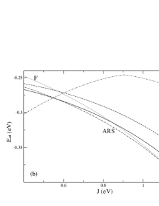
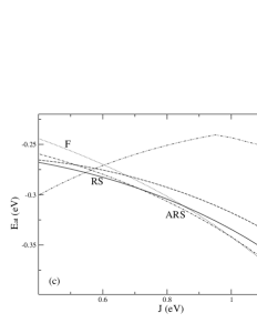
Figures 5$(a)$ and $(b)$ show a plot of $E_{V}^{\prime}$ as a function of $J$ for all these magnetic phases. Notice that for fixed $\Delta_{t}$, $E_{V}^{\prime}$ depends only on the ratio $J/U_{2}$ and scales like $\tau^{2}/U_{2}$, if $\tau$ is the largest hopping integral in the basal plane.

FIG. 5.: The energy gain $E^{\prime}_{V}$ per V atom as a function of $J$ for different spin configurations (AF, RS, ARS and F type), represented by dashed, solid, dot-dashed and dotted lines, respectively. In panel (a) the hopping parameters are the standard ones (Mattheiss set), while in panel (b) the set considered by Mila et al. is used ($\tau=0.27$ and all others hopping integrals equal to zero.)

One general feature that is apparent from these figures and the next Fig. 7 is that the stability region for the RS phase is very much reduced in the two parameter space of the hopping integrals and the ratio $J/U_{2}$, in contrast with the spin $S=1/2$ case. [7] The AF and F phases occupy nearly all phase space in such a way that $J/U_{2}\approx 0.4$ almost marks the transition from a stable antiferromagnetic in-plane spin structure to a ferromagnetic one (see, for example, Fig. 5$(a)$). This behavior depends on the fact that for low $J$ values, the system wants to maximize the number of electron jumps (which occur more easily in an AF structure) to the detriment of on-site Hund’s energy gain, whereas for high $J$ values this last mechanism is prevalent. In between, in a small range of $J/U_{2}$ slightly depending on the values of the hopping integrals, typically $0.30<J/U_{2}<0.45$, find their place the RS and the ARS phases, each occupying about half of the interval. Even in the most favorable case (see Fig. 5$(b)$), their stabilization energy, due to the competing presence of the AF and F phases, is very small, of the order of 2 meV, to be compared with a transition temperature corresponding to 15 meV. Even though the stabilization energy scales like $\tau^{2}/U_{2}$, there is not enough room to improve substantially the situation by a reasonable variation of the parameters.

More specifically, we see from Fig. 5($a$) that assuming Mattheiss’ parameters for the hopping integrals we achieve a stable solution for the RS structure only for a very small window of the ratio $J/U_{2}$ around $0.4$. The most favorable situation for this latter is obtained with the choice made by Mila et al.,[19] by putting $\alpha=\beta=\sigma=0$ and $\tau\neq 0$ (Fig. 5$(b)$), but even in this case, as already stated, the stabilization energy is of the order of $\approx 2$ meV. We have also tried to investigate the role of the monoclinic distortion in stabilizing the RS structure. To introduce it, we have assumed that after the setting in of the broken symmetry phase, the hopping parameters $\chi=t^{12}$ and $\theta=t^{13}$ take a value different from zero along the bond $\delta_{1}$, whose length increases by 0.1 Å, and remain substantially zero along the other two directions, where the bond distance is unchanged after the transition. The result is essentially negative as there is a little but not significant improvement.

Turning now to the orbital structure, Fig. 6$(a)$ gives the minimizing values of the orbital mixing angles $\psi_{n}$ of Eq. (142) in the basal plane at all molecular sites for the RS configurations found in Fig. 5. The value $\psi_{n}=0$ for all sites means a uniform occupation throughout the crystal of the molecular state $\|\psi_{-}\rangle$, i.e., the ferro-orbital solution found by Mila et al.[19] In agreement with them, also for the ARS configuration (their A phase) we find a uniform solution with a minimizing angle $\psi_{n}=\pi/2$, i.e., a uniform occupation throughout the crystal of the molecular state $\|\psi_{+}\rangle$.

Moreover for the AF and F phases we find a continuum of orbital degeneracies of antiferro-orbital type, in the sense that all the orbital configurations with any mixing angle $\psi_{a}$ on the central molecule and a mixing angle of $\psi_{a}+\pi/2$ on the three in-plane neighboring molecules, have the same energy (see Fig. 6$(b)$ for the particular case $\psi_{a}=0$). This feature can also be deduced analytically from Eq. (184).

As anticipated in Section IV, the magnetic group of the ferro-orbital solution is not in keeping with the experimental findings of Goulon et al.[21] We have therefore analyzed the orbital order of the excited configurations within a range of $\simeq$ 4 meV from the ground state. Referring to Fig. 5$(b)$, for $J=0.85$ meV, the ferro-orbital RS(FO) phase is at $E^{\prime}_{V}=-0.0744$ meV, all the degenerate AF(AO) phases with antiferro-orbital ordering at $E^{\prime}_{V}=-0.0729$ meV and a phase that will be called RS(ME), for reasons that will shortly become apparent (ME stands for magneto-electric), with the orbital ordering depicted in Fig. 5$(c)$ lies at $E^{\prime}_{V}=-0.0707$.

We have also explored the consequences of varying the ratio $\alpha/\tau$ from the zero value assumed in Fig. 5$(b)$ to about one. From the picture following Eq. (121) it is in fact evident that an $\alpha=t_{11}$ value of the same order of $\tau=t_{23}$ would favor an antiferro-orbital coupling along the $\delta_{1}$ bond in the RS phase.

FIG. 6.: The angles indicate the orbital occupancy of the vertical molecule at a given site. $(a)$ Orbital ordering in the RS(FO) phase. $(b)$ Orbital ordering in the RS(AO) phase. $(c)$ Orbital ordering in the RS(ME) excited phase.

FIG. 7.: Phase diagram in the ($\alpha/\tau$, $J/U_{2}$) parameter plane. Here AF, F, ARS denote the corresponding type of magnetic order; RS and RS’ denote the RS(FO) and RS(AO) phase with orbital structures shown in Fig. 6. The solid lines indicate the phase boundaries. We put for simplicity $\beta=\sigma=0$.

To this purpose we have drawn the phase diagram for the various magnetic configurations in the plane $\alpha/\tau$ versus $J/U_{2}$. The relevant result is shown in Fig. 7. As expected another RS’ phase with the same spin configuration as the RS phase appears, centered around the values $\alpha/\tau=0.7$ and $J/U_{2}=0.40$, with the molecular orbital ordering depicted in Fig. 6$(b)$ (in-plane antiferro-orbital (AO) ordering). Again an energy analysis of the excited phases for $J=1.0$ eV and $\alpha=-0.19$ eV leads to the following sequency:

$$E^{\prime}_{V}[RS(AO)] = -0.0909~{}{\rm eV}$$

$$E^{\prime}_{V}[AF(AO)] = -0.0908~{}{\rm eV}$$

$$E^{\prime}_{V}[RS(ME)] = -0.0905~{}{\rm eV}$$

where in brackets we have indicated the spin and orbital configurations. As seen, the energy spreading is now much more reduced, only 0.4 meV separating the orbital ME phase from the ground state.

In order to establish the magnetic group for the RS phases, of interest here, we observe that, because of the entangled nature of the molecular state, the average orbital type of the two atoms constituting the vertical pair is the same. With respect to the $D_{3d}$ corundum symmetry point group, the state $|0\rangle$ transforms according to the totally symmetric representation ($A_{1g}$ in Schoenflies notation) while $|-1\rangle$ and $|1\rangle$ are partner functions of the bidimensional $E_{g}$ representation and transform, respectively, like the basis $e^{(1)}_{g}$ and $e^{(2)}_{g}$ in CNR.[7, 8]

We can then use Table I to see which symmetry operations conserve the colored magnetic structure, obtained by adding to the lattice sites not only a spin label but also a color label given by the type of orbital occupation at that site. We find that the magnetic group for the RS(AO) phase is $C_{2}\otimes\hat{T}$ (group n. 4 in Section IV), whereas that for the RS(ME) phase is $C_{2h}(C_{s})$ (group n. 7). Therefore the only phase compatible with the findings of Goulon et al. [21] is this latter. As it will be argued in Section VII, it might be possible that the combined effect of the symmetry breaking of the spin and orbital degrees of freedom lead to a favorable coupling to the lattice in such a way as to stabilize the RS(ME) phase with respect to the competing configurations. In this case the role of the monoclinic distortion would be essential to achieve the ground state with the correct symmetry.

B The case of the atomic variational state.

Even though the values of the hopping parameters as shown in Table III seem to favor what we called the molecular regime, nonetheless we think it could be useful to analyze, for the sake of completeness, also the other regime. In this case the orbital on-site part of the variational wave function is atomic-like and should be written as

$$\parallel\psi^{o}_{i}\rangle=\cos\theta_{i}|0\rangle_{i}+\sin\theta_{i}(\cos\psi_{i}|1\rangle_{i}+\sin\psi_{i}|-1\rangle_{i})~{},$$ (190)

allowing all the three states $|0\rangle_{i}$, $|1\rangle_{i}$ and $|-1\rangle_{i}$ to be present without any a priori restriction on their relative weight, contrary to the molecular case. The relative weight of the three states is then determined through the minimization procedure with respect to the variational parameters $\theta_{i}$ and $\psi_{i}$. The only restriction we impose is that the solutions must fill the whole crystal, with a periodicity not less than that of the monoclinic cell. This is indeed a quite reasonable request, as the solutions with periodicity of more than the unit cell should describe excited states. As the unit cell of V₂O₃ is formed by 8 V atoms, there are in principle 16 minimization angles. In order to simplify the problem, we use the symmetry relations between the variational angles dictated by all the possible magnetic space groups for V₂O₃ described in section IV. Indeed for each group, the states of the V atoms inside the cell are not independent, but are related by the symmetry operations, thus providing a reduction of the number of parameters. By taking the absolute minimum we shall determine the orbital and spin nature of the ground state, together with the corresponding magnetic group. In this way we exclude solutions not invariant with respect to the chosen groups, but we note that all the interesting subgroups for V₂O₃ have been taken into account.

Table IV. Number of independent variational angles in the unit cell according to the various possible magnetic groups.

$$\begin{array}[]{llll}1.&\hat{E},\hat{I},\hat{C}_{2},\hat{\sigma}_{b}&\Rightarrow&({\rm V}_{1},{\rm V}_{2},{\rm V}_{6},{\rm V}_{8})\equiv(\theta_{1},\psi_{1})\\ &&&({\rm V}_{3},{\rm V}_{4},{\rm V}_{5},{\rm V}_{7})\equiv(\theta_{2},\psi_{2})\\ 2.&\hat{E},\hat{I},\hat{T},\hat{T}\hat{I}&\Rightarrow&({\rm V}_{1},{\rm V}_{2},{\rm V}_{3},{\rm V}_{7})\equiv(\theta_{1},\psi_{1})\\ &&&({\rm V}_{4},{\rm V}_{5},{\rm V}_{6},{\rm V}_{8})\equiv(\theta_{2},\psi_{2})\\ 3.&\hat{E},\hat{I},\hat{T}\hat{C}_{2},\hat{T}\hat{\sigma}_{b}&\Rightarrow&({\rm V}_{1},{\rm V}_{2},{\rm V}_{4},{\rm V}_{5})\equiv(\theta_{1},\psi_{1})\\ &&&({\rm V}_{3},{\rm V}_{6},{\rm V}_{7},{\rm V}_{8})\equiv(\theta_{2},\psi_{2})\\ 4.&\hat{E},\hat{T},\hat{C}_{2},\hat{T}\hat{C}_{2}&\Rightarrow&({\rm V}_{1},{\rm V}_{4},{\rm V}_{7},{\rm V}_{8})\equiv(\theta_{1},\psi_{1})\\ &&&({\rm V}_{2},{\rm V}_{3},{\rm V}_{5},{\rm V}_{6})\equiv(\theta_{2},\psi_{2})\\ 5.&\hat{E},\hat{C}_{2},\hat{T}\hat{I},\hat{T}\hat{\sigma}_{b}&\Rightarrow&({\rm V}_{1},{\rm V}_{3},{\rm V}_{5},{\rm V}_{8})\equiv(\theta_{1},\psi_{1})\\ &&&({\rm V}_{2},{\rm V}_{4},{\rm V}_{6},{\rm V}_{7})\equiv(\theta_{2},\psi_{2})\\ 6.&\hat{E},\hat{T},\hat{\sigma}_{b},\hat{T}\hat{\sigma}_{b}&\Rightarrow&({\rm V}_{1},{\rm V}_{5},{\rm V}_{6},{\rm V}_{7})\equiv(\theta_{1},\psi_{1})\\ &&&({\rm V}_{2},{\rm V}_{3},{\rm V}_{4},{\rm V}_{8})\equiv(\theta_{2},\psi_{2})\\ 7.&\hat{E},\hat{\sigma}_{b},\hat{T}\hat{I},\hat{T}\hat{C}_{2}&\Rightarrow&({\rm V}_{1},{\rm V}_{3},{\rm V}_{4},{\rm V}_{6})\equiv(\theta_{1},\psi_{1})\\ &&&({\rm V}_{2},{\rm V}_{5},{\rm V}_{7},{\rm V}_{8})\equiv(\theta_{2},\psi_{2})\\ 8.&C_{2h}\otimes\hat{T}&\Rightarrow&{\rm~{}same~{}for~{}all~{}V_{i}}\equiv(\theta,\psi)\end{array}$$ (206)

In Table IV we list, for each magnetic group, the number of independent angles associated with the corresponding atomic sites. This number is obviously given by 16 divided the order of the group.

Given the full expression for $H_{\rm eff}$ reported in Appendix C, we can then evaluate the matrix elements for $H^{F}_{\rm eff}$ and $H^{A}_{\rm eff}$ (as defined by Eqs. (78) and (79)) along vertical ($\delta_{4}$) and horizontal ($\delta_{1},\delta_{2},\delta_{3}$) bonds. The spin averages are again calculated and included in the formulas as in the previous subsection.

In the case of $H^{F}_{\rm eff}$ the matrix element for the $\delta_{4}$ bond is:

$$\begin{array}[]{l}\langle\Psi_{b}|\langle\Psi_{a}|H_{\rm eff}^{F}(\delta_{4})|\Psi_{a}\rangle|\Psi_{b}\rangle=\\ (\cos^{2}\theta_{a}\sin^{2}\theta_{b}+\sin^{2}\theta_{a}\cos^{2}\theta_{b})\tilde{G}_{1}\\ +\sin^{2}\theta_{a}\sin^{2}\theta_{b}(\cos^{2}\psi_{a}\sin^{2}\psi_{b}+\sin^{2}\psi_{a}\cos^{2}\psi_{b})\tilde{G}_{2}\\ +\sin^{2}\theta_{a}\sin^{2}\theta_{b}\sin 2\psi_{a}\sin 2\psi_{b}\tilde{G}_{3}\\ +\sin 2\theta_{a}\sin 2\theta_{b}(\cos\psi_{a}\cos\psi_{b}+\sin\psi_{a}\sin\psi_{b})\tilde{G}_{4}~{},\end{array}$$ (212)

where

$$\begin{array}[]{l}\tilde{G}_{1}=u(\mu^{2}+\rho^{2})\\ \tilde{G}_{2}=2u\mu^{2}\\ \tilde{G}_{3}=-u\mu^{2}\\ \tilde{G}_{4}=-u\mu\rho\\ u=-\frac{1}{U_{2}-J}~{}.\end{array}$$ (219)

For $H^{A}_{\rm eff}$ it can be written as

$$\begin{array}[]{l}\langle\Psi_{b}|\langle\Psi_{a}|H_{\rm eff}^{A}(\delta_{4})|\Psi_{a}\rangle|\Psi_{b}\rangle=\\ \cos^{2}\theta_{a}\cos^{2}\theta_{b}\tilde{F}_{1}\\ +(\cos^{2}\theta_{a}\sin^{2}\theta_{b}+\sin^{2}\theta_{a}\cos^{2}\theta_{b})\tilde{F}_{2}\\ +\sin^{2}\theta_{a}\sin^{2}\theta_{b}\tilde{F}_{3}\\ +\sin^{2}\theta_{a}\sin^{2}\theta_{b}(\cos^{2}\psi_{a}\cos^{2}\psi_{b}+\sin^{2}\psi_{a}\sin^{2}\psi_{b})\tilde{F}_{4}\\ +\sin^{2}\theta_{a}\sin^{2}\theta_{b}(\cos^{2}\psi_{a}\sin^{2}\psi_{b}+\sin^{2}\psi_{a}\cos^{2}\psi_{b})\tilde{F}_{5}\\ +\sin^{2}\theta_{a}\sin^{2}\theta_{b}\sin 2\psi_{a}\sin 2\psi_{b}\tilde{F}_{6}\\ +\sin 2\theta_{a}\sin 2\theta_{b}(\cos\psi_{a}\cos\psi_{b}+\sin\psi_{a}\sin\psi_{b})\tilde{F}_{7}~{},\end{array}$$ (228)

where

$$\begin{array}[]{l}\tilde{F}_{1}=2(v+w)\mu^{2}\\ \tilde{F}_{2}=(v+\frac{5w}{3})\mu^{2}+\frac{2w}{3}\rho^{2}\\ \tilde{F}_{3}=(v+w)\rho^{2}\\ \tilde{F}_{4}=(v+\frac{7w}{3})\mu^{2}\\ \tilde{F}_{5}=\frac{4w}{3}\mu^{2}\\ \tilde{F}_{6}=(\frac{v}{2}-\frac{w}{6})\mu^{2}\\ \tilde{F}_{7}=(\frac{v}{2}-\frac{w}{6})\mu\rho\\ v=-\frac{1}{U_{2}+4J}\\ w=-\frac{1}{U_{2}+2J}~{}.\end{array}$$ (239)

For the horizontal bond $\delta_{1}$, the $H^{F}_{\rm eff}$ average value takes the form:

$$\begin{array}[]{l}\langle\Psi_{c}|\langle\Psi_{a}|H_{\rm eff}^{F}(\delta_{1})|\Psi_{a}\rangle|\Psi_{c}\rangle\\ =[\sin^{2}\theta_{a}\cos^{2}\psi_{a}(\cos^{2}\theta_{c}+\sin^{2}\theta_{c}\sin^{2}\psi_{c})\\ +\sin^{2}\theta_{c}\cos^{2}\psi_{c}(\cos^{2}\theta_{a}+\sin^{2}\theta_{a}\sin^{2}\psi_{a})]\bar{G}_{1}\\ +[\sin^{2}\theta_{a}\sin^{2}\psi_{a}(\cos^{2}\theta_{c}+\sin^{2}\theta_{c}\cos^{2}\psi_{c})\\ +\sin^{2}\theta_{c}\sin^{2}\psi_{c}(\cos^{2}\theta_{a}+\sin^{2}\theta_{a}\cos^{2}\psi_{a})]\bar{G}_{2}\\ +[2\cos^{2}\theta_{a}\cos^{2}\theta_{c}+\sin^{2}\theta_{a}\cos^{2}\psi_{a}\cos^{2}\theta_{c}\\ +\cos^{2}\theta_{a}\sin^{2}\theta_{c}\cos^{2}\psi_{c}+\sin^{2}\theta_{a}\sin^{2}\theta_{c}(\sin^{2}\psi_{a}\\ +\sin^{2}\psi_{c})-\sin 2\theta_{a}\sin 2\theta_{c}\sin\psi_{a}\sin\psi_{c}]\bar{G}_{3}\\ +\sin^{2}\theta_{a}\sin^{2}\theta_{c}\sin 2\psi_{a}\sin 2\psi_{c}\bar{G}_{4}\\ +\sin 2\theta_{a}\sin 2\theta_{c}\cos\psi_{a}\cos\psi_{c}\bar{G}_{5}\\ +(\sin 2\theta_{a}\sin^{2}\theta_{c}\cos\psi_{a}\sin 2\psi_{c}\\ +\sin 2\theta_{c}\sin^{2}\theta_{a}\cos\psi_{c}\sin 2\psi_{a})\bar{G}_{6}\\ +\sin 2\theta_{a}\sin 2\theta_{c}\sin\psi_{a}\sin\psi_{c}\bar{G}_{7}\\ +(\cos^{2}\theta_{a}\sin^{2}\theta_{c}+\cos^{2}\theta_{c}\sin^{2}\theta_{a})\bar{G}_{8}\\ +(\cos^{2}\theta_{a}\sin 2\theta_{c}\sin\psi_{c}\\ +\cos^{2}\theta_{c}\sin 2\theta_{a}\sin\psi_{a})\bar{G}_{9}\\ +[\sin 2\theta_{a}\sin\psi_{a}(\cos^{2}\theta_{c}+\sin^{2}\theta_{c}\cos 2\psi_{c})\\ +\sin 2\theta_{c}\sin\psi_{c}(\cos^{2}\theta_{a}+\sin^{2}\theta_{a}\cos 2\psi_{a})]\bar{G}_{10}~{},\end{array}$$ (258)

where

$$\begin{array}[]{l}\bar{G}_{1}=u\alpha^{2}\\ \bar{G}_{2}=u\beta^{2}\\ \bar{G}_{3}=u\tau^{2}\\ \bar{G}_{4}=u\alpha\beta\\ \bar{G}_{5}=u\alpha\sigma\\ \bar{G}_{6}=-u\alpha\tau\\ \bar{G}_{7}=-u\beta\sigma\\ \bar{G}_{8}=u\sigma^{2}\\ \bar{G}_{9}=-u\sigma\tau\\ \bar{G}_{10}=u\beta\tau~{}.\end{array}$$ (269)

For the same bond in the case of $H^{A}_{\rm eff}$ we obtain:

$$\begin{array}[]{l}\langle\Psi_{c}|\langle\Psi_{a}|H_{\rm eff}^{A}(\delta_{1})|\Psi_{a}\rangle|\Psi_{c}\rangle=\\ \cos^{2}\theta_{a}\cos^{2}\theta_{c}\bar{F}_{1}\\ +(\cos^{2}\theta_{a}\sin^{2}\theta_{c}\sin^{2}\psi_{c}+\sin^{2}\theta_{a}\cos^{2}\theta_{c}\sin^{2}\psi_{a})\bar{F}_{2}\\ +(\cos^{2}\theta_{a}\sin^{2}\theta_{c}+\sin^{2}\theta_{a}\cos^{2}\theta_{c})\bar{F}_{3}\\ +\sin^{2}\theta_{a}\sin^{2}\theta_{c}(\cos^{2}\psi_{a}\sin^{2}\psi_{c}+\sin^{2}\psi_{a}\cos^{2}\psi_{c})\bar{F}_{4}\\ +\sin^{2}\theta_{a}\sin^{2}\theta_{c}\bar{F}_{5}\\ +\sin^{2}\theta_{a}\sin^{2}\theta_{c}(\cos^{2}\psi_{a}+\cos^{2}\psi_{c})\bar{F}_{6}\\ +\sin^{2}\theta_{a}\sin^{2}\theta_{c}\sin 2\psi_{a}\sin 2\psi_{c}\bar{F}_{7}\\ +\sin 2\theta_{a}\sin 2\theta_{c}\sin\psi_{a}\sin\psi_{c}\bar{F}_{8}\\ +(\sin^{2}\theta_{a}\sin 2\theta_{c}\sin 2\psi_{a}\cos\psi_{c}\\ +\sin^{2}\theta_{c}\sin 2\theta_{a}\sin 2\psi_{c}\cos\psi_{a})\bar{F}_{9}\\ +\sin 2\theta_{a}\sin 2\theta_{c}\cos\psi_{a}\cos\psi_{c}\bar{F}_{10}\\ +[\sin 2\theta_{a}\sin\psi_{a}(1+\sin^{2}\theta_{c}\sin^{2}\psi_{c})\\ +\sin 2\theta_{c}\sin\psi_{c}(1+\sin^{2}\theta_{a}\sin^{2}\psi_{a})]\bar{F}_{11}\\ +[\sin 2\theta_{a}\sin\psi_{a}(2-\sin^{2}\theta_{c})\\ +\sin 2\theta_{c}\sin\psi_{c}(2-\sin^{2}\theta_{a})]\bar{F}_{12}~{},\end{array}$$ (286)

with the definitions

$$\begin{array}[]{l}\bar{F}_{1}=v(\alpha^{2}+\beta^{2})+\frac{w}{3}(3(\alpha^{2}+\beta^{2})+5\tau^{2})\\ \bar{F}_{2}=v(-\alpha^{2}+\beta^{2})+\frac{w}{3}(\alpha^{2}-\beta^{2}-2\tau^{2})\\ \bar{F}_{3}=v(\alpha^{2}+\tau^{2})+\frac{w}{3}(2\alpha^{2}+3\beta^{2}+2\sigma^{2}+5\tau^{2})\\ \bar{F}_{4}=v(\alpha^{2}+\beta^{2})+\frac{1}{6}(\alpha^{2}+\beta^{2})\\ \bar{F}_{5}=v\sigma^{2}+\frac{w}{3}(3\alpha^{2}+\sigma^{2}+5\tau^{2})\\ \bar{F}_{6}=v\tau^{2}+\frac{w}{6}(-3\alpha^{2}+3\beta^{2}+2\tau^{2})\\ \bar{F}_{7}=(-\frac{v}{2}+\frac{w}{6})\alpha\beta\\ \bar{F}_{8}=\frac{v}{2}(\beta\sigma+\tau^{2})-\frac{w}{6}(\beta\sigma+\tau^{2})\\ \bar{F}_{9}=-(\frac{v}{2}-\frac{w}{6})\alpha\tau\\ \bar{F}_{10}=-(\frac{v}{2}-\frac{w}{6})\alpha\sigma\\ \bar{F}_{11}=-\frac{w}{3}\beta\tau\\ \bar{F}_{12}=-\frac{w}{3}\sigma\tau~{}.\par\end{array}$$ (300)

The matrix elements along $\delta_{2}$ and $\delta_{3}$ are easily derived from the expressions (258)-(300) using the symmetry properties of $H_{\rm eff}$ under the trigonal $C_{3}$ symmetry, as done previously in the molecular case.

In this way the average of the Hamiltonian on a ferromagnetic bond is given by the sole $H_{\rm eff}^{F}$ contribution, while for an antiferromagnetic bond we have to add $\frac{1}{3}H_{\rm eff}^{F}$ to the contribution of $H_{\rm eff}^{A}$.

The term due to the trigonal field splitting (80) can be also taken into account. Its energy contribution per V-atom is given by: $\frac{\Delta_{t}}{8}\sum_{i=1}^{8}\sin^{2}{\theta_{i}}$.

Given all these ingredients, we can now evaluate the ground state energy for all 8 groups: the “true” ground state energy per V atom, $E_{at}$, is then obtained as the absolute minimum among the 8 minima, determining in this way also the magnetic group for V₂O₃. The results are presented for two choices of hopping parameters corresponding to those of Fig. 5$(a)$, $(b)$ in the molecular regime and $\rho=-0.82$ and $\mu=0.2$ eV (Mattheiss set, see Table III). We consider for the moment only the case $\Delta_{t}=0$. As apparent from Fig. 8$(a)$, $(b)$, we have in the atomic regime one more curve (labeled VAF) giving the ground state energy of the system in a magnetic configuration in which the two atoms along $\delta_{4}$ are coupled antiferromagnetically, independently of all the other spin couplings along $\delta_{1}$, $\delta_{2}$ and $\delta_{3}$. Of course, such ground state configuration was absent in the molecular regime, where we started from a $S^{M}=2$ state. It relates to the $S^{M}=0$ molecular solution in Fig. 3.

Notice that a direct comparison between Fig. 5 and Fig. 8 may be misleading, since in the atomic regime the vertical bond $\delta_{4}$ is included in the ground state energy $E_{at}$, while in the molecular regime we have subtracted from $E_{V}$ the binding energy of the molecule: $\frac{\Delta E_{m}}{2}$. This means that the energy $\frac{\Delta E_{m}}{2}$ ($\simeq-0.33~{}eV$, for $J\simeq 1.0$)) must be added to $E^{\prime}_{V}$ of Fig. 5, thus restoring the correct numerical correspondence between the two cases.

In particular, for values of $J$ such that the VAF is not the stable phase, we can write the atomic ground state energy per V atom as

$$E_{at}=E^{\prime}_{at}-\frac{1}{2}\frac{\rho^{2}+\mu^{2}}{U_{2}-J}~{},$$ (301)

where we separated the in-plane contribution $E^{\prime}_{at}$ from the energy gain along $\delta_{4}$, i.e., $-\frac{1}{2}\frac{\rho^{2}+\mu^{2}}{U_{2}-J}$.

In this way, dropping all the common Hartree-Fock terms along the vertical bond $\delta_{4}$, we can write the two inequalities:

$$\left\{\begin{array}[]{l}E^{\prime}_{at}<E^{\prime}_{V}\\[8.5359pt] E^{\prime}_{at}>E^{\prime}_{V}-\frac{\rho\mu}{U_{2}-J}~{}.\end{array}\right.$$ (304)

The reason for these inequalities is the following. The first of Eqs. (304) says that the in-plane energy gain with the atomic variational wave functions is always lower than the corresponding molecular one. This is to be expected, since the variational space in the molecular case is reduced with respect to the atomic one, where the states are not constraint to satisfy the form of Eq. (121).

The second of Eqs. (304) states, instead, that the molecular ground state lies lower than the atomic one, because of the correlation energy. Note that, while the first Equation is always valid, the validity of the second is limited to sufficiently high values of $\rho$ and $\mu$ (for example, the standard set) and its breakdown marks the transition point between the molecular and the atomic regime.

FIG. 8.: The ground state energy $E_{at}$ as a function of $J$ for different magnetic configurations. The hopping parameters are taken as follows: (a) $\rho=-0.82$, $\mu=0.2$, $\alpha=0.14$, $\beta=-0.05$, $\sigma=0.05$, $\tau=0.27$; (b) $\rho=-0.82$, $\mu=0.2$, $\alpha=0$, $\beta=0$, $\sigma=0$, $\tau=0.27$; (c) $\rho=-0.82$, $\mu=0$, $\alpha=0.14$, $\beta=-0.05$, $\sigma=0.05$, $\tau=0.27$.

The analysis of the two Figs. 8$(a)$, $(b)$ shows that the RS phase is realized in both cases (though in Fig. 8$(b)$ it is very small). Indeed in the case of the standard set of parameters, the atomic solution is even more stable than the corresponding molecular one, the first excited state lying $\simeq 3$ meV above. Nonetheless it cannot be considered a good ground state solution for the reasons stated above (see Eqs. (304)). Moreover, the magnetic space group of the solution is not ME, being group 2. of Table IV. The orbital pattern is made of planes of V-atoms, orthogonal to the $c_{H}$-axis, in $|0\rangle$ state, alternating with planes of V atoms in $|-1\rangle$ state.

Figure 8$(c)$ presents the case $\rho=-0.82$ eV and $\mu=0$ eV, in order to satisfy the criterion for using an atomic variational function, i.e., the correlation energy less than the in-plane exchange energy. In fact, in this case the condition $\mu=0$ implies that the second of Eqs. (304) is not satisfied, and then $E_{at}<E_{V}$. Thus the RS solution obtained in this case is the overall ground state of the system for this value of the parameters. Unfortunately, this solution has the usual drawbacks already analyzed (stability energy of only $3$ meV, space magnetic group 2. of Table IV, not ME) and moreover the ME solution lies very far from the ground state ($\simeq 100$ meV), thus confirming the fact that the choice $\mu=0$ is not suitable to describe V₂O₃.

The effect of the crystal field in this situation is to favor the occupancy of the $|0\rangle$ states on all the atoms, as expected. In the case of high trigonal distortion $\Delta_{t}=0.4$ eV, we obtain (not shown) a direct transition from the VAF to the F phase, with no stable RS solution. In VAF phase, all the V atoms are in the $|0\rangle$ configuration, while in the F phase, the percentage of $|0\rangle$ states lowers to $85\%$, the remaining $15\%$ being essentially $|1\rangle$, to allow the hopping process.

Note that even in the case of such a high value of the trigonal distortion ($\Delta_{t}=0.4$ eV), we checked that the molecular phase is by far the more stable state (for example, for the standard set of parameters and $J=1.0$ eV, the molecular ground state lies 60 meV lower than the atomic one).

VII Discussion and conclusions.

In this concluding section we shall review the implications of the spin $S=1$ model for V₂O₃ described above in relation to the present experimental evidence. The comparison will allow us to focus on merits and drawbacks of the various solutions obtained in the previous section.

A Occupancy of $a_{1g}$ orbital and spin.

In the molecular regime, the variational wave function was assumed to be of the form given in Eq. (146), in which the occupancy of the $a_{1g}$ orbital is 25%. However Park et al.[14] report an occupancy of 17% for this orbital in the AFI phase. This is an indication that other states with only $e_{g}$ occupancy are mixed in the ground state of this phase. In reality, even though the state in Eq. (146) is the main component of the wave function, in doing the variational procedure we have neglected excited states of the vertical molecule lying within the range of the exchange energy in the basal plane. Now, since for all the RS phases the ratio $J/U_{2}$ is around $0.35\div 0.40$, our study of the vertical molecule in section V-B (see Fig. (4)) shows that we should take $\Delta_{t}$ around $0.4$ eV if we want to stabilize the ferromagnetic coupling and find excited states with only $e_{g}$ occupancy close enough to the ground state. Fig. 4$(d)$ illustrates the level structure in the case $J=1.0$ eV, from which one can infer that two more states with $S^{M}=1$ and $S^{M}=0$ can be mixed with the $S^{M}=2$ wave function. Notice from Fig. 3$(d)$ that for $J=0.85$ eV these states are even closer to the $S^{M}=2$ ground state. A more general calculation will be done in the future. We can however estimate in an approximate way the amount of mixing by writing the variational state $|\Psi\rangle=\alpha|S^{M}=2\rangle+\beta|S^{M}=1\rangle+\gamma|S^{M}=0\rangle$ and imposing the condition that the average value of the molecular spin be 1.7, as derived from neutrons and non magnetic resonant scattering data (see Introduction). Therefore

$$2\alpha^{2}+1\beta^{2}+0\gamma^{2}=1.7~{},$$

which, together with the normalization condition $\alpha^{2}~{}+~{}\beta^{2}~{}+~{}\gamma^{2}~{}=~{}1$, gives

$$\alpha^{2}=0.85-\beta^{2}/2~{}~{};~{}~{}\gamma^{2}=0.15-\beta^{2}/2~{}.$$

In the situation shown in Fig. 4$(c)$, even the small spin-orbit interaction of the AFI phase of V₂O₃ ($\simeq 25~{}meV$), which couples only to $S^{M}=1,2$ states and not with $S^{M}=0$ state, can make the ground state energies for $S^{M}=1$ and $S^{M}=0$ comparable. This means that we can reasonably take $\beta^{2}=\gamma^{2}$, thus obtaining $\alpha^{2}=0.8$ and $\beta^{2}=\gamma^{2}=0.1$. Therefore the $a_{1g}$ orbital occupancy reduces to $0.8\times 25\%=20\%$, in good agreement with Park et al.[14] findings. This means that also Park’s findings point to a value of the trigonal distortion around $0.4$ eV.

B Trigonal distortion.

In CNR[7] the trigonal distortion $\Delta_{t}$ in the corundum phase (and therefore also in the monoclinic phase, since the cage of the oxygens remains almost unaltered at the metal to insulator transition [3]) was assumed to be negligible, in keeping with the suggestion by Rubistein.[34] This latter was based on the following experimental evidence in the paramagnetic phases of V₂O₃:

• There is no detectable anisotropy in the Knight shift of the NMR spectrum;

• There is no observable quadrupole splitting in the NMR spectrum.

• Zero anisotropy was observed in single-crystal susceptibility measurements for various crystalline orientations with respect to the magnetic field. A large value for $\Delta_{t}$ would result in highly anisotropic Van Vleck susceptibility.

However the theoretical estimate by Ezhov et al.[16] and the previous discussion on the $a_{1g}$ occupancy seem to point out to a value of $\Delta_{t}$ around $0.4$ eV. The problem is how to reconcile this high value with the above experimental findings. The concept of an entangled state for the vertical pair described by the wave function in Eq. (121) solves this apparent inconsistency in an elegant way. Indeed, the short range magnetic fluctuations observed by neutron scattering experiments [6] in the paramagnetic phases imply a statistical occupancy of the two orbitally degenerate molecular states of Eq. (121) and x-ray absorption spectra [14] show evidence of an average 25% occupancy of the $a_{1g}$ and 75% of $e_{g}$ orbitals. This is very near to the totally symmetric occupation of the three orbitals (1/3 each), restoring in such a way the cubic symmetry. Notice that in a static picture the conclusion of a negligible trigonal distortion would be unescapable.

C Monoclinic distortion.

In their work Mila et al.[19] point out that the ferro-orbital molecular ordering found for the C phase (our RS(FO)) causes an effective uniaxial stress on the lattice degrees of freedom, leading to a uniform rotation of the vertical V-V pairs, in agreement with the monoclinic distortion proposed by Dernier and Marezio.[3] At first sight this explanation seems convincing. However on second thought it is not clear why atoms of two adjacent vertical pairs belonging to the same basal plane (e.g., V₁ and V₂, or V₄ and V₅ with reference to Fig. 1) should go on opposite sides of the line joining them (x-axis in the figure). Since the two V atoms with their local oxygen environment are on average in the same electronic state, the initial displacive force should have the same sign along the x-axis, by an application of the Feynman theorem to an Hamiltonian depending on parameters (in this case the position coordinates of the V atoms). While a posteriori we see that the lattice energy is lowered if the two atoms move toward the oxygen voids, the initial drive should go on the correct direction. This is indeed what happens if one assume the orbital ordering found in the RS(ME) phase. The two atoms in the basal plane are in different electronic states, one odd with respect to the operation x $\rightarrow$ $-$x (state $|\psi^{o}_{-}\rangle$) and the other even (state $|\psi^{o}_{+}\rangle$), and this situation is reproduced for each pair of atoms in the basal planes throughout the crystal.

We observe that in the RS(ME) phase the stress arising from the magnetostrictive forces due to the broken symmetry of the spin degrees of freedom and the one originating from the orbital coupling to the lattice, presenting the same pattern of broken symmetry, act along the same axis, in contrast to the other two phases. This fact might give an advantage to the RS(ME) spin-orbital configuration in its coupling to the lattice so as to become stabilized with respect to them. In such an instance the monoclinic distortion would be essential to achieve the ground state with the correct symmetry indicated by the Goulon experiment. Clearly more investigation is needed on this point.

D Anomalous diffraction.

In their paper Mila et al.[19] claim that the ferro-orbital ordering they propose, while different from that invoked by Paolasini et al.[13], is also consistent with the experimental findings. However we feel that their argument was rather scant and we try to present here a more in depth analysis of the implications of X-ray resonant scattering data, deferring a more complete treatment to a future work. We shall see that the space magnetic symmetry group of the AFI ground state plays an essential role in the discussion of the structure factor, since it can discriminate among different theoretical models.

In the anomalous diffraction at the V K-edge, the structure factor $F$ is given by

$$F=\sum_{n}f_{n}e^{i\vec{Q}\cdot\vec{R_{n}}}$$ (305)

where the sum is performed over the eight V-atoms of the unit cell, $f_{n}$ is the resonant atomic scattering factor (RASF), $\vec{Q}$ the momentum transfer at the chosen given reflection and $\vec{R}_{n}$ the atomic position inside the cell.

We follow the numbering of V atoms as given in Fig. 1, and divide the eight atoms in the monoclinic unit cell into two groups with opposite orientation of the magnetic moment, $4\;(u,v,w),\;5\;(-u,-v,-w),\;2\;(1/2+u,-v,w),\;1\;(1/2-u,v,-w)$, and 8, 6, 3, 7, with coordinates obtained by adding the vector (1/2, 1/2, 1/2) to the first group. Here $u=0.3438,\;v=0.0008,\;w=0.2991$ are the fractional coordinates of the atoms in unit of the monoclinic axis[3] and the origin is taken between the atoms V₄ and V₅ in the same basal plane. It is important to note for the following discussion that the bc monoclinic unit cell (space group $I2/a$) is not primitive, so that, neglecting the magnetic moments, the two groups of atoms with their oxygen environment are translationally equivalent.

At the $(h,k,l)$ monoclinic reflection, putting for brevity $b=e^{i\pi(h+k+l)}$, and $\phi^{\pm}=2\pi(hu\pm hv+lw)$, the structure factor F in Eq. (305) can be written as

$$F = {\bigg{[}}(f_{8}+bf_{4})e^{i\phi^{+}}+(f_{6}+bf_{5})e^{-i\phi^{+}}{\bigg{]}}$$ (306)

$$+ b(-1)^{h}{\bigg{[}}(f_{2}+bf_{3})e^{i\phi^{-}}+(f_{1}+bf_{7})e^{-i\phi^{-}}{\bigg{]}}$$ (307)

The RASF $f_{n}$’s in this equation are tensorial quantities given by the following expression[35]:

$$f_{n}(\omega)=\sum_{m}\frac{<1s|O^{\dagger}|\Psi_{m}><\Psi_{m}|O|1s>}{\hbar\omega+E_{1s}-E_{m}-i\Gamma_{n}/2}$$ (308)

The transition operator $O$ is the electronic part of $\vec{\epsilon}\cdot\vec{r}(1+i\vec{k}\cdot\vec{r})$ with the usual notation for the photon energy $\omega$, the polarization $\vec{\epsilon}$ and the propagation vector $\vec{k}$, so that $f_{n}(\omega)$ may bear two, three or four Cartesian indices according to dipole-dipole (DD), dipole-quadrupole (DQ) and quadrupole-quadrupole (QQ) transitions. Then the atomic scattering amplitude is obtained by saturating with the appropriate $\vec{\epsilon}$ and $\vec{k}$ components.

We can now use the operations of the magnetic symmetry group of the crystal to transform the $f_{n}$’s into one another. In doing so we remember that a symmetry operation changes the site index according to Table I of Section IV and simultaneously acts on the tensor components. This action reduces to a multiplicative factor $\pm 1$ since $\hat{I}^{2}=\hat{C}_{2}^{2}=\hat{\sigma}_{b}^{2}=\hat{T}^{2}=E$. Thus $\hat{I}f_{n}=f_{n}$ for DD, QQ and $\hat{I}f_{n}=-f_{n}$ for DQ transitions. Moreover, we find it expedient to split the RASF tensor into a symmetric (charge) part and an antisymmetric (magnetic) part[35]: $f_{n}=f^{+}_{n}+f^{-}_{n}$. In this way, $\hat{T}f_{n}^{\pm}=\pm f_{n}^{\pm}$. Notice that in establishing the site correspondence and the transformation properties of the tensor components it is essential that the Wannier functions of adjacent hexagonal planes be defined as in CNR[8] (Eqs. (2.4) and (2.7)), i.e., they should be related by the same symmetry operation connecting the sites. For example, since the sites 2 and 4 are related by the glide plane $\hat{\sigma}_{b}$, the definition of the Wannier function at site 2 should be obtained from that at site 4 by changing $y$ into $-y$, if we take the reference frame as depicted in Fig. 1.

Consider now the magnetic group $C_{2h}\otimes\hat{T}$, which is appropriate to the ferro-orbital AFI phase of V₂O₃ as proposed by Mila et al.[19] Defining $A(\phi^{\pm})=(e^{i\phi^{\pm}}+\hat{I}e^{-i\phi^{\pm}})$ and using the symmetry operation $\hat{I}$ to connect sites 5 and 6 to 4 and 8, and sites 1 and 7 to 2 and 3, and the operation $\hat{T}\hat{\sigma}_{b}$ to connect sites 2 and 3 to 4 and 8, we can express the structure factor as:

$$F_{hkl} = [A(\phi^{+})+A(\phi^{-})(-1)^{h}\hat{T}\hat{\sigma}_{b}](f_{8}^{+}+bf_{4}^{+})$$ (309)

$$+ [A(\phi^{+})+A(\phi^{-})(-1)^{h}\hat{T}\hat{\sigma}_{b}](f_{8}^{-}+bf_{4}^{-})$$ (310)

Using now the peculiar fact that in V₂O₃ $v\approx 0$, defining $\phi=2\pi(hu+lw)$ and $A(\phi^{\pm})\equiv A(\phi)$ and remembering that $\hat{T}f_{n}^{\pm}=\pm f_{n}^{\pm}$, we finally obtain:

$$F_{hkl} = (e^{i\phi}+\hat{I}e^{-i\phi})[1+(-1)^{h}\hat{\sigma}_{b}](f_{8}^{+}+bf_{4}^{+})$$ (311)

$$+ (e^{i\phi}+\hat{I}e^{-i\phi})[1-(-1)^{h}\hat{\sigma}_{b}](f_{8}^{-}+bf_{4}^{-})$$ (312)

In this expression we assume that the operators have already acted on the site indices, so that they should act only on the tensor components. We notice that, considering the $f_{n}$ as scalars, we recover the crystallographic extinction rules (the reflections with $h+k+l$ odd ($b=-1$) are lattice forbidden) and the selection rules for non resonant magnetic scattering (for $b=-1$, those with $h$ even are magnetically allowed, those with $h$ odd are forbidden). The classification by Paolasini et al.[13] of the lattice forbidden reflections into purely orbital and purely magnetic was actually based on the non resonant magnetic scattering and might therefore be only approximate.

Returning to the resonant regime at lattice forbidden reflections with $h$ odd, one can easily see from Eq. (312) that there cannot be any charge (and therefore orbital) signal if sites 8 and 4 are in the same orbital state, since they are completely equivalent from the point of view of the lattice. Therefore what Mila et al.[19] are really saying is that the (1,1,1) reflection observed by Paolasini et al. can only be of purely magnetic origin, which however has nothing to do with orbital ordering.

A similar argument is also valid for the $C_{2}\otimes{\hat{T}}$ symmetry of the RS(AO) phase. In this case, using ${\hat{T}}$ and ${\hat{C}_{2}}$ to relate the various sites, as shown in Table I, we obtain:

$$F_{hkl} = (e^{i\phi}+b(-1)^{h}{\hat{C}}_{2}e^{-i\phi})(b+1)(f_{3}^{+}+b(-1)^{h}f_{4}^{+})$$ (313)

$$+ (e^{i\phi}-b(-1)^{h}{\hat{C}}_{2}e^{-i\phi})(b-1)(f_{3}^{-}+b(-1)^{h}f_{4}^{-})$$ (314)

(315)

and again it is impossible to observe a charge scattering when $b=-1$.

We believe however that the claim made by Paolasini et al. for evidence of orbital ordering has some substance, despite their approximate classification. Indeed it is well known that the magnetic part of the tensor for DD transition is only active in the $\sigma-\pi$ channel and its imaginary part can be shown to be proportional to the magnetic circular dichroism in absorption. At the K-edge this latter is proportional to $\langle L\rangle$, the average of the orbital momentum operator in the final state. [36, 37] Due to the fact that in V₂O₃ the moment lies [4] on the glide plane, a reflection with respect to this plane change the sign of $\langle L\rangle$, so that $\hat{\sigma}f_{n}^{-}(DD)=-f_{n}^{-}(DD)$. This implies, from Eq. (312), that the DD tensor is magnetically active only at reflections with $h$ even, but cannot contribute at $h$ odd. The experimental evidence from Paolasini et al. [13, 22] is in keeping with this conclusion except for the observed intensity at 5464 eV, corresponding to $1s\rightarrow 3d$ transitions, where at both types of reflections ($h$ even and $h$ odd) signals of comparable magnitude were detected.

Notice that we expect a strong contribution from the DD transitions at this energy for $h$ even, since the V-atoms are off-center with respect to the oxygen octahedra, which are furthermore distorted. At the same time, the ratio of the transition matrix elements between DD and DQ transitions in the case of V₂O₃ is estimated by Fabrizio et al. [12] to be of the order of 7, in good agreement with the experimental data by Goulon et al.[21]. Therefore the observed comparable intensities at 5464 eV for reflections with $h$ even and odd cannot have the same magnetic origin. This argument also invalidates the explanation proposed by Lovesey et al.[38] that the (1,1,1) signal is due to the octupolar component of the QQ transition, a tensor of rank 3, apart from problems related to its use of an approximate symmetry. At this reflection the signal should indeed be much smaller than at an allowed DD magnetic reflection ($h$ even). Therefore much more work is needed to establish the exact implications of the resonant diffraction experiment on the nature of the AFI ground state of V₂O₃, since this complex question cannot be dismissed by too simple arguments.

If we now consider the reduced group $C_{2h}(C_{s})$, using $\hat{T}\hat{I}$ and $\hat{\sigma}_{b}$ to relate the various sites, again according to Table I, we find for the scattering factor :

$$F_{hkl} = (e^{i\phi}+b\hat{T}\hat{I}e^{-i\phi})[1+b(-1)^{h}\hat{\sigma}_{b}](f_{8}+bf_{4})$$ (316)

$$= (e^{i\phi}+b\hat{I}e^{-i\phi})[1+b(-1)^{h}\hat{\sigma}_{b}](f_{8}^{+}+bf_{4}^{+})$$ (317)

$$+ (e^{i\phi}-b\hat{I}e^{-i\phi})[1+b(-1)^{h}\hat{\sigma}_{b}](f_{8}^{-}+bf_{4}^{-})$$ (318)

At reflections forbidden by the lattice ($b=-1$), the charge scattering behavior of expressions (312), (315) and (318) is substantially different. As already emphasized in the case of the two groups $C_{2h}\otimes\hat{T}$ and $C_{2}\otimes\hat{T}$ there cannot be charge scattering, while for $C_{2h}(C_{s})$, $f_{8}^{+}$ is different from $f_{4}^{+}$, so that a charge signal might appear. In particular this is the case for the orbitally ordered state RS(ME), due to the different molecular states of the molecules straddling atoms 8-7 and 4-1. This fact would readily explain the comparable intensity observed at reflections with $h$ even and odd, since the transition is always dipolar in nature, and stronger than that due to DQ or QQ processes. Again more work is needed to establish whether the predictions of the ground state proposed here for V₂O₃ are in keeping with the experimental findings.

Finally we want to point out that the RS(AO) configuration, due to the orbital ordering, can give rise to magnetic reflections of dipolar character, with $b=-1$ and $h$ even or odd, as apparent from Eq. (315), since atoms 3 and 4 belong to vertical pairs in different molecular states. However this phase cannot be an eligible candidate for being the ground state of V₂O₃, due to the presence of $\hat{T}$ in the associated space magnetic group, that forbids magnetoelectricity.

E Conclusions.

In this paper we have derived the strong coupling limit of an Hubbard Hamiltonian with three degenerate $t_{2g}$ states containing two electrons coupled to spin $S=1$, and have re-examined the low-temperature ground-state properties of V₂O₃. Given the present experimental evidence in favor of a spin-1 state of the V³⁺-ions, there is no doubt that the original suggestion by J. Allen, [20] later taken up and developed by Mila et al.[19], that the vertical molecules constitute the building blocks of this compound in all three phases of the phase diagram, is the key concept to understand the physics of the phase transitions observed in V₂O₃. In fact the molecular unit reconciles the existence of orbital degeneracy, required to explain experimental evidence ranging from inelastic neutron scattering data to the relaxation time of the nuclear spins in NMR studies, with the spin-1 state of the V³⁺-ions. Focusing on the AFI phase and analyzing the parameter space of the problem, we have indeed found that one has to consider two regimes, depending on the relative size of the intramolecular correlation energy and the in-plane exchange energy. These two regimes dictate the form of the variational wave function. In both cases we found minimizing solutions in a reduced region of the Hamiltonian parameters (hopping integrals versus $\frac{J}{U_{2}}$) with the real spin configuration. The molecular solutions are more suited to explain certain experimental facts, like, for example, the lack of detectable anisotropy in various spectroscopies in the paramagnetic phases of V₂O₃. However there remain two orders of problems which will require future investigation.

The first one is the rather small stability region in the phase space of the parameters $\frac{\alpha}{\tau}$ versus $\frac{J}{U_{2}}$ and the small stabilization energy of the RS phases compared to neighboring competing configurations (in the range $1.5\div 2$ meV, using the standard set of parameters). The AF(AO) phase, with its continuum degeneracy and the in-plane spin-orbital antiferromagnetic coupling with trigonal symmetry, is very reminiscent of the paramagnetic insulating (PI) phase at higher temperature, setting aside the short range of the correlations.[6] Therefore one would expect an energy gap at least of the order of the transition temperature (15 meV), and we know[6] that the estimated Neel temperature of the AFI phase is about 20 meV. The problem shows up again if one tries to calculate the exchange integrals for spin wave excitations. Even though, looking at Fig. 5(b), one can find a value of Hund parameter $J$ such that the exchange integrals along $\delta_{1}$ is ferromagnetic and about half the one antiferromagnetic along $\delta_{2}$ or $\delta_{3}$, as found by inelastic neutron scattering measurements,[39] their actual values are off by a factor of five. Moreover it does not seem that longer range hopping parameters, neglected in our calculations, might cure this drawback. Since the energy scale is set by $\frac{\tau^{2}}{U_{2}}$, in order to get the energetics correct one should increase $\tau$ by more than a factor of two. However this would be an easy way to escape a problem that has more profound roots. We tend to believe in fact that the difficulty stems from the mean field treatment of this highly correlated electron system on one side and on the other side from the neglect of the lattice degrees of freedom.

The second order of problems regards the consistency of the RS phases with the experimental findings of x-ray synchrotron radiation spectroscopies, namely the anomalous diffraction and non-reciprocal x-ray gyrotropy. We have argued that the comparable intensity of the observed signal at the Vanadium K-edge in resonant diffraction at both reflections with $h$ even and odd cannot be interpreted as being purely magnetic in origin, but finds a natural explanation if one assume that the ground state magnetic symmetry group is such as to allow charge scattering, i.e., if there is the appropriate orbital ordering. This group is the same as the one indicated by the non-reciprocal spectroscopy. However none of the stable RS phases found admit this group, so that they only allow resonant magnetic scattering. This is the reason that prompted us to indicate the excited configurations RS(ME) as possible candidates for the correct ground state of the AFI phase, invoking an optimal coupling with the lattice degrees of freedom. This assignment makes also a definite prediction for a transverse magneto-electric effect in this phase which could be subjected to experimental test.

A The effective Hamiltonian in terms of fermion operators.

Here we report the results of the calculations performed to derive the effective Hamiltonian in terms of the fermion operators.

The explicit form of the projection operators $X^{(i)}_{j}$, ($i=1,2,3$) defined in Eqs. (29), (31) is given by:

$$X^{(1)}=\sum_{\sigma}\bigg{[}n_{1\sigma}n_{2\sigma}n_{3\sigma}+\frac{1}{3}(n_{1\sigma}n_{2\sigma}n_{3{\bar{\sigma}}}+n_{1\sigma}n_{2{\bar{\sigma}}}n_{3\sigma}+n_{1{\bar{\sigma}}}n_{2\sigma}n_{3\sigma})+\frac{1}{3}\sum_{{m,m^{\prime},m^{\prime\prime}}\atop{m\neq m^{\prime}\neq m^{\prime\prime}}}n_{m\sigma}c_{m^{\prime}\sigma}^{+}c_{m^{\prime}{\bar{\sigma}}}c^{+}_{m^{\prime\prime}{\bar{\sigma}}}c_{m^{\prime\prime}\sigma}\bigg{]}$$ (A1)

$$X^{(2)}=\sum_{\sigma}\bigg{[}\frac{1}{2}\sum_{m,m^{\prime}\neq m}n_{m\sigma}n_{m^{\prime}\sigma}n_{m^{\prime}{\bar{\sigma}}}-\sum_{{m,m^{\prime},m^{\prime\prime}}\atop{m\neq m^{\prime}\neq m^{\prime\prime}}}n_{m\sigma}c_{m^{\prime}\sigma}^{+}c_{m^{\prime}{\bar{\sigma}}}^{+}c_{m^{\prime\prime}{\bar{\sigma}}}c_{m^{\prime\prime}\sigma}$$ (A2)

$$+\frac{2}{3}(n_{1\sigma}n_{2\sigma}n_{3{\bar{\sigma}}}+n_{1\sigma}n_{2{\bar{\sigma}}}n_{3\sigma}+n_{1{\bar{\sigma}}}n_{2\sigma}n_{3\sigma})-\frac{1}{3}\left(n_{1\sigma}(c_{2\sigma}^{+}c_{2{\bar{\sigma}}}c_{3{\bar{\sigma}}}^{+}c_{3\sigma}+c_{3\sigma}^{+}c_{3{\bar{\sigma}}}c_{2{\bar{\sigma}}}^{+}c_{2\sigma})\right.$$ (A3)

$$+n_{2\sigma}(c_{1\sigma}^{+}c_{1{\bar{\sigma}}}\left.c_{3{\bar{\sigma}}}^{+}c_{3\sigma}+c_{3\sigma}^{+}c_{3{\bar{\sigma}}}c_{1{\bar{\sigma}}}^{+}c_{1\sigma})+n_{3\sigma}(c_{1\sigma}^{+}c_{1{\bar{\sigma}}}c_{2{\bar{\sigma}}}^{+}c_{2\sigma}+c_{2\sigma}^{+}c_{2{\bar{\sigma}}}c_{1{\bar{\sigma}}}^{+}c_{1\sigma})\right)\bigg{]}$$ (A4)

$$X^{(3)}=\frac{1}{2}\sum_{\sigma}\sum_{{m,m^{\prime}\neq m}\atop{m^{\prime\prime}\neq m}}n_{m\sigma}c_{m^{\prime}\sigma}^{+}c_{m^{\prime}{\bar{\sigma}}}^{+}c_{m^{\prime\prime}{\bar{\sigma}}}c_{m^{\prime\prime}\sigma}$$ (A5)

For simplicity we omitted the site index as all operators act on site $j$.

Dividing $H_{\rm eff}$ into three parts, according to the $X^{(i)}$ definitions, we obtain the following expressions:

$$H_{\rm eff}^{(1)}=-\frac{1}{U_{2}-J}\sum_{ij\sigma}\sum_{nn^{\prime}}\sum_{mm^{\prime}m^{\prime\prime}}(1-\delta_{mm^{\prime}})(1-\delta_{mm^{\prime\prime}})(1-\delta_{m^{\prime}m^{\prime\prime}})c^{+}_{in\sigma}c_{in^{\prime}\sigma}$$ (A6)

$$\times{\bigg{[}}t_{ij}^{nm}t_{ji}^{mn^{\prime}}n_{jm^{\prime}\sigma}n_{jm^{\prime\prime}\sigma}-t_{ij}^{nm}t_{ji}^{m^{\prime}n^{\prime}}c_{jm^{\prime}\sigma}^{+}c_{jm\sigma}n_{jm^{\prime\prime}\sigma}{\bigg{]}}$$ (A7)

$$-\frac{1}{3(U_{2}-J)}\sum_{ij\sigma}\sum_{nn^{\prime}}\sum_{mm^{\prime}m^{\prime\prime}}(1-\delta_{mm^{\prime}})(1-\delta_{mm^{\prime\prime}})(1-\delta_{m^{\prime}m^{\prime\prime}})$$ (A8)

$$\times{\bigg{[}}t_{ij}^{nm}t_{ji}^{mn^{\prime}}(c_{in\sigma}^{+}c_{in^{\prime}\sigma}n_{jm^{\prime}\sigma}n_{jm^{\prime\prime}{\bar{\sigma}}}+\frac{1}{2}c_{in{\bar{\sigma}}}^{+}c_{in^{\prime}{\bar{\sigma}}}n_{jm^{\prime}\sigma}n_{jm^{\prime\prime}\sigma})$$ (A9)

$$-t_{ij}^{nm}t_{ji}^{m^{\prime}n^{\prime}}(c_{in\sigma}^{+}c_{in^{\prime}\sigma}c_{jm^{\prime}\sigma}^{+}c_{jm\sigma}n_{jm^{\prime\prime}{\bar{\sigma}}}+c_{in\sigma}^{+}c_{in^{\prime}{\bar{\sigma}}}c_{jm^{\prime}{\bar{\sigma}}}^{+}c_{jm\sigma}n_{jm^{\prime\prime}\sigma}+c_{in{\bar{\sigma}}}^{+}c_{in^{\prime}\sigma}c_{jm^{\prime}\sigma}^{+}c_{jm{\bar{\sigma}}}n_{jm^{\prime\prime}\sigma}){\bigg{]}}$$ (A10)

$$-\frac{1}{3(U_{2}-J)}\sum_{ij\sigma}\sum_{nn^{\prime}}\sum_{mm^{\prime}m^{\prime\prime}}(1-\delta_{mm^{\prime}})(1-\delta_{mm^{\prime\prime}})(1-\delta_{m^{\prime}m^{\prime\prime}})$$ (A11)

$$\times{\bigg{[}}t_{ij}^{nm}t_{ji}^{mn^{\prime}}{\big{(}}c_{in\sigma}^{+}c_{in^{\prime}\sigma}c_{jm^{\prime}\sigma}^{+}c_{jm^{\prime}{\bar{\sigma}}}c_{jm^{\prime\prime}{\bar{\sigma}}}^{+}c_{jm^{\prime\prime}\sigma}+c_{in\sigma}^{+}c_{in^{\prime}{\bar{\sigma}}}n_{jm^{\prime}\sigma}c_{jm^{\prime\prime}{\bar{\sigma}}}^{+}c_{jm^{\prime\prime}\sigma}+c_{in{\bar{\sigma}}}^{+}c_{in^{\prime}\sigma}c_{jm^{\prime}\sigma}^{+}c_{jm^{\prime}{\bar{\sigma}}}n_{jm^{\prime\prime}\sigma}{\big{)}}$$ (A12)

$$-t_{ij}^{nm}t_{ji}^{m^{\prime}n^{\prime}}{\big{(}}c_{in\sigma}^{+}c_{in^{\prime}\sigma}c_{jm^{\prime}{\bar{\sigma}}}^{+}c_{jm\sigma}c_{jm^{\prime\prime}\sigma}^{+}c_{jm^{\prime\prime}{\bar{\sigma}}}+c_{in\sigma}^{+}c_{in^{\prime}\sigma}c_{jm^{\prime}{\bar{\sigma}}}^{+}c_{jm{\bar{\sigma}}}n_{jm^{\prime\prime}\sigma}+c_{in\sigma}^{+}c_{in^{\prime}\sigma}c_{jm^{\prime}\sigma}^{+}c_{jm{\bar{\sigma}}}c_{jm^{\prime\prime}{\bar{\sigma}}}c_{jm^{\prime\prime}\sigma}$$ (A13)

$$+c_{in\sigma}^{+}c_{in^{\prime}{\bar{\sigma}}}c_{jm^{\prime}\sigma}^{+}c_{jm\sigma}c_{jm^{\prime\prime}{\bar{\sigma}}}^{+}c_{jm^{\prime\prime}\sigma}+c_{in{\bar{\sigma}}}^{+}c_{in^{\prime}\sigma}c_{jm^{\prime}\sigma}^{+}c_{jm{\sigma}}c_{jm^{\prime\prime}\sigma}^{+}c_{jm^{\prime\prime}{\bar{\sigma}}}+c_{in{\bar{\sigma}}}^{+}c_{in^{\prime}{\bar{\sigma}}}c_{jm^{\prime}\sigma}^{+}c_{jm\sigma}n_{jm^{\prime\prime}\sigma}{\big{)}}{\bigg{]}}$$ (A14)

$$H_{\rm eff}^{(2)}=-\frac{1}{2(U_{2}+2J)}\sum_{ij\sigma}\sum_{nn^{\prime}}\sum_{mm^{\prime}}(1-\delta_{mm^{\prime}}){\bigg{[}}t_{ij}^{nm}t_{ji}^{mn^{\prime}}(c^{+}_{in\sigma}c_{in^{\prime}\sigma}n_{jm{\bar{\sigma}}}n_{jm^{\prime}\sigma}+c^{+}_{in{\bar{\sigma}}}c_{in^{\prime}{\bar{\sigma}}}n_{jm\sigma}n_{jm^{\prime}\sigma}$$ (A15)

$$-c^{+}_{in\sigma}c_{in^{\prime}{\bar{\sigma}}}c^{+}_{jm{\bar{\sigma}}}c_{jm\sigma}n_{jm^{\prime}\sigma}-c^{+}_{in{\bar{\sigma}}}c_{in^{\prime}\sigma}c^{+}_{jm\sigma}c_{jm{\bar{\sigma}}}n_{jm^{\prime}\sigma}{\bigg{]}}+\frac{1}{2(U_{2}+2J)}\sum_{ij\sigma}\sum_{nn^{\prime}}\sum_{mm^{\prime}m^{\prime\prime}}(1-\delta_{mm^{\prime}})(1-\delta_{mm^{\prime\prime}})(1-\delta_{m^{\prime}m^{\prime\prime}})$$ (A16)

$$\times{\bigg{[}}t_{ij}^{nm}t_{ji}^{m^{\prime}n^{\prime}}(c^{+}_{in\sigma}c_{in^{\prime}\sigma}c^{+}_{jm{\bar{\sigma}}}c_{jm^{\prime}{\bar{\sigma}}}n_{jm^{\prime\prime}\sigma}-c^{+}_{in\sigma}c_{in^{\prime}{\bar{\sigma}}}c^{+}_{jm{\bar{\sigma}}}c_{jm^{\prime}\sigma}n_{jm^{\prime\prime}\sigma}$$ (A17)

$$-c^{+}_{in{\bar{\sigma}}}c_{in^{\prime}\sigma}c^{+}_{jm\sigma}c_{jm^{\prime}{\bar{\sigma}}}n_{jm^{\prime\prime}\sigma}+c^{+}_{in{\bar{\sigma}}}c_{in^{\prime}{\bar{\sigma}}}c^{+}_{jm\sigma}c_{jm^{\prime}\sigma}n_{jm^{\prime\prime}\sigma}){\bigg{]}}$$ (A18)

$$-\frac{2}{3(U_{2}+2J)}\sum_{ij\sigma}\sum_{nn^{\prime}}\sum_{mm^{\prime}\atop{m^{\prime\prime}}}(1-\delta_{mm^{\prime}})(1-\delta_{mm^{\prime\prime}})(1-\delta_{m^{\prime}m^{\prime\prime}}){\bigg{[}}t_{ij}^{nm}t_{ji}^{mn^{\prime}}(c_{in\sigma}^{+}c_{in^{\prime}\sigma}n_{jm^{\prime}\sigma}n_{jm^{\prime\prime}{\bar{\sigma}}}+\frac{1}{2}c_{in{\bar{\sigma}}}^{+}c_{in^{\prime}{\bar{\sigma}}}n_{jm^{\prime}\sigma}n_{jm^{\prime\prime}\sigma})$$ (A19)

$$-t_{ij}^{nm}t_{ji}^{m^{\prime}n^{\prime}}(c_{in\sigma}^{+}c_{in^{\prime}\sigma}c_{jm^{\prime}\sigma}^{+}c_{jm\sigma}n_{jm^{\prime\prime}{\bar{\sigma}}}+c_{in\sigma}^{+}c_{in^{\prime}{\bar{\sigma}}}c_{jm^{\prime}{\bar{\sigma}}}^{+}c_{jm\sigma}n_{jm^{\prime\prime}\sigma}+c_{in{\bar{\sigma}}}^{+}c_{in^{\prime}\sigma}c_{jm^{\prime}\sigma}^{+}c_{jm{\bar{\sigma}}}n_{jm^{\prime\prime}\sigma}){\bigg{]}}$$ (A20)

$$+\frac{1}{3(U_{2}+2J)}\sum_{ij\sigma}\sum_{nn^{\prime}}\sum_{mm^{\prime}m^{\prime\prime}}(1-\delta_{mm^{\prime}})(1-\delta_{mm^{\prime\prime}})(1-\delta_{m^{\prime}m^{\prime\prime}}){\bigg{[}}t_{ij}^{nm}t_{ji}^{mn^{\prime}}{\big{(}}c_{in\sigma}^{+}c_{in^{\prime}\sigma}c_{jm^{\prime}\sigma}^{+}c_{jm^{\prime}{\bar{\sigma}}}c_{jm^{\prime\prime}{\bar{\sigma}}}^{+}c_{jm^{\prime\prime}\sigma}$$ (A21)

$$+c_{in\sigma}^{+}c_{in^{\prime}{\bar{\sigma}}}n_{jm^{\prime}\sigma}c_{jm^{\prime\prime}{\bar{\sigma}}}^{+}c_{jm^{\prime\prime}\sigma}+c_{in{\bar{\sigma}}}^{+}c_{in^{\prime}\sigma}c_{jm^{\prime}\sigma}^{+}c_{jm^{\prime}{\bar{\sigma}}}n_{jm^{\prime\prime}\sigma}{\big{)}}-t_{ij}^{nm}t_{ji}^{m^{\prime}n^{\prime}}{\big{(}}c_{in\sigma}^{+}c_{in^{\prime}\sigma}c_{jm^{\prime}{\bar{\sigma}}}^{+}c_{jm\sigma}c_{jm^{\prime\prime}\sigma}^{+}c_{jm^{\prime\prime}{\bar{\sigma}}}$$ (A22)

$$+c_{in\sigma}^{+}c_{in^{\prime}\sigma}c_{jm^{\prime}{\bar{\sigma}}}^{+}c_{jm{\bar{\sigma}}}n_{jm^{\prime\prime}\sigma}+c_{in\sigma}^{+}c_{in^{\prime}\sigma}c_{jm^{\prime}\sigma}^{+}c_{jm{\bar{\sigma}}}c_{jm^{\prime\prime}{\bar{\sigma}}}c_{jm^{\prime\prime}\sigma}+c_{in\sigma}^{+}c_{in^{\prime}{\bar{\sigma}}}c_{jm^{\prime}\sigma}^{+}c_{jm\sigma}c_{jm^{\prime\prime}{\bar{\sigma}}}c_{jm^{\prime\prime}\sigma}$$ (A23)

$$+c_{in{\bar{\sigma}}}^{+}c_{in^{\prime}\sigma}c_{jm^{\prime}\sigma}^{+}c_{jm{\bar{\sigma}}}c_{jm^{\prime\prime}\sigma}c_{jm^{\prime\prime}{\bar{\sigma}}}+c_{in\sigma}^{+}c_{in^{\prime}{\bar{\sigma}}}c_{jm^{\prime}\sigma}^{+}c_{jm\sigma}n_{jm^{\prime\prime}\sigma}{\big{)}}{\bigg{]}}$$ (A24)

$$H_{\rm eff}^{(3)}=-\frac{1}{2(U_{2}+4J)}\sum_{ij\sigma}\sum_{nn^{\prime}}\sum_{mm^{\prime}}(1-\delta_{mm^{\prime}}){\bigg{[}}t_{ij}^{nm}t_{ji}^{mn^{\prime}}(c^{+}_{in\sigma}c_{in^{\prime}\sigma}n_{jm{\bar{\sigma}}}n_{jm^{\prime}\sigma}+c^{+}_{in{\bar{\sigma}}}c_{in^{\prime}{\bar{\sigma}}}n_{jm\sigma}n_{jm^{\prime}\sigma}$$ (A25)

$$-c^{+}_{in\sigma}c_{in^{\prime}{\bar{\sigma}}}c^{+}_{jm{\bar{\sigma}}}c_{jm\sigma}n_{jm^{\prime}\sigma}-c^{+}_{in{\bar{\sigma}}}c_{in^{\prime}\sigma}c^{+}_{jm\sigma}c_{jm{\bar{\sigma}}}n_{jm^{\prime}\sigma}{\bigg{]}}-\frac{1}{2(U_{2}+4J)}\sum_{ij\sigma}\sum_{nn^{\prime}}\sum_{mm^{\prime}m^{\prime\prime}}(1-\delta_{mm^{\prime}})(1-\delta_{mm^{\prime\prime}})(1-\delta_{m^{\prime}m^{\prime\prime}})$$ (A26)

$$\times{\bigg{[}}t_{ij}^{nm}t_{ji}^{m^{\prime}n^{\prime}}(c^{+}_{in\sigma}c_{in^{\prime}\sigma}c^{+}_{jm{\bar{\sigma}}}c_{jm^{\prime}{\bar{\sigma}}}n_{jm^{\prime\prime}\sigma}-c^{+}_{in\sigma}c_{in^{\prime}{\bar{\sigma}}}c^{+}_{jm{\bar{\sigma}}}c_{jm^{\prime}\sigma}n_{jm^{\prime\prime}\sigma}$$ (A27)

$$-c^{+}_{in{\bar{\sigma}}}c_{in^{\prime}\sigma}c^{+}_{jm\sigma}c_{jm^{\prime}{\bar{\sigma}}}n_{jm^{\prime\prime}\sigma}+c^{+}_{in{\bar{\sigma}}}c_{in^{\prime}{\bar{\sigma}}}c^{+}_{jm\sigma}c_{jm^{\prime}\sigma}n_{jm^{\prime\prime}\sigma}){\bigg{]}}$$ (A28)

B Commutation relations.

In the following we evaluate the commutators used to derive the effective Hamiltonian in section II.

As usual, given two generic operators A and B, we define $[A,B]\equiv AB-BA$ and $\{A,B\}\equiv AB+BA$

$$\begin{array}[]{l}[n_{m\sigma}n_{m^{\prime}\sigma^{\prime}}n_{m^{\prime\prime}\sigma^{\prime\prime}},c^{+}_{m^{\prime\prime\prime}\sigma^{\prime\prime\prime}}]=\delta_{mm^{\prime\prime\prime}}\delta_{\sigma\sigma^{\prime\prime\prime}}c^{+}_{m\sigma}n_{m^{\prime}\sigma^{\prime}}n_{m^{\prime\prime}\sigma^{\prime\prime}}\\ +\delta_{m^{\prime}m^{\prime\prime\prime}}\delta_{\sigma^{\prime}\sigma^{\prime\prime\prime}}n_{m\sigma}c^{+}_{m^{\prime}\sigma^{\prime}}n_{m^{\prime\prime}\sigma^{\prime\prime}}+\delta_{m^{\prime\prime}m^{\prime\prime\prime}}\delta_{\sigma^{\prime\prime}\sigma^{\prime\prime\prime}}n_{m\sigma}n_{m^{\prime}\sigma^{\prime}}c^{+}_{m^{\prime\prime}\sigma^{\prime\prime}}\end{array}$$ (B3)

$$\begin{array}[]{l}\{c_{m^{\prime\prime\prime\prime}\sigma^{\prime\prime\prime\prime}},[n_{m\sigma}n_{m^{\prime}\sigma^{\prime}}n_{m^{\prime\prime}\sigma^{\prime\prime}},c^{+}_{m^{\prime\prime\prime}\sigma^{\prime\prime\prime}}]\}=\delta_{mm^{\prime\prime\prime\prime}}\delta_{\sigma\sigma^{\prime\prime\prime\prime}}{\big{(}}\delta_{mm^{\prime\prime\prime}}\delta_{\sigma\sigma^{\prime\prime\prime}}n_{m^{\prime}\sigma^{\prime}}n_{m^{\prime\prime}\sigma^{\prime\prime}}\\ +\delta_{m^{\prime}m^{\prime\prime\prime}}\delta_{\sigma^{\prime}\sigma^{\prime\prime\prime}}c_{m\sigma}c^{+}_{m^{\prime}\sigma^{\prime}}n_{m^{\prime\prime}\sigma^{\prime\prime}}+\delta_{m^{\prime\prime}m^{\prime\prime\prime}}\delta_{\sigma^{\prime\prime}\sigma^{\prime\prime\prime}}c_{m\sigma}n_{m^{\prime}\sigma^{\prime}}c^{+}_{m^{\prime\prime}\sigma^{\prime\prime}}{\big{)}}\\ +\delta_{m^{\prime}m^{\prime\prime\prime\prime}}\delta_{\sigma^{\prime}\sigma^{\prime\prime\prime\prime}}{\big{(}}\delta_{m^{\prime\prime}m^{\prime\prime\prime}}\delta_{\sigma^{\prime\prime}\sigma^{\prime\prime\prime}}n_{m\sigma}c_{m^{\prime}\sigma^{\prime}}c^{+}_{m^{\prime\prime}\sigma^{\prime\prime}}+\delta_{m^{\prime}m^{\prime\prime\prime}}\delta_{\sigma^{\prime}\sigma^{\prime\prime\prime}}n_{m\sigma}n_{m^{\prime\prime}\sigma^{\prime\prime}}\\ -\delta_{mm^{\prime\prime\prime}}\delta_{\sigma\sigma^{\prime\prime\prime}}c^{+}_{m\sigma}c_{m^{\prime}\sigma^{\prime}}n_{m^{\prime\prime}\sigma^{\prime\prime}}{\big{)}}+\delta_{m^{\prime\prime}m^{\prime\prime\prime\prime}}\delta_{\sigma^{\prime\prime}\sigma^{\prime\prime\prime\prime}}{\big{(}}\delta_{m^{\prime\prime}m^{\prime\prime\prime}}\delta_{\sigma^{\prime\prime}\sigma^{\prime\prime\prime}}n_{m\sigma}n_{m^{\prime}\sigma^{\prime}}\\ -\delta_{m^{\prime}m^{\prime\prime\prime}}\delta_{\sigma^{\prime}\sigma^{\prime\prime\prime}}n_{m\sigma}c^{+}_{m^{\prime}\sigma^{\prime}}c_{m^{\prime\prime}\sigma^{\prime\prime}}-\delta_{mm^{\prime\prime\prime}}\delta_{\sigma\sigma^{\prime\prime\prime}}c^{+}_{m\sigma}n_{m^{\prime}\sigma^{\prime}}c_{m^{\prime\prime}\sigma^{\prime\prime}}{\big{)}}\end{array}$$ (B9)

$$\begin{array}[]{l}[n_{m^{\prime\prime}\sigma^{\prime\prime}}c^{+}_{m\sigma}c_{m^{\prime}\sigma}c^{+}_{m^{\prime}\bar{\sigma}}c_{m\bar{\sigma}},c^{+}_{m^{\prime\prime\prime}\sigma^{\prime\prime\prime}}]=\delta_{m^{\prime\prime}m^{\prime\prime\prime}}\delta_{\sigma^{\prime\prime}\sigma^{\prime\prime\prime}}c^{+}_{m^{\prime\prime}\sigma^{\prime\prime}}c^{+}_{m\sigma}c_{m^{\prime}\sigma}c^{+}_{m^{\prime}\bar{\sigma}}c_{m\bar{\sigma}}\\ +n_{m^{\prime\prime}\sigma^{\prime\prime}}c^{+}_{m\sigma}c^{+}_{m^{\prime}\sigma^{\prime}}(\delta_{m^{\prime}m^{\prime\prime\prime}}\delta_{\sigma\sigma^{\prime\prime\prime}}c_{m\bar{\sigma}}-\delta_{mm^{\prime\prime\prime}}\delta_{\bar{\sigma}\sigma^{\prime\prime\prime}}c_{m^{\prime}\sigma})\end{array}$$ (B12)

$$\begin{array}[]{l}\{c_{m^{\prime\prime\prime\prime}\sigma^{\prime\prime\prime\prime}},[n_{m^{\prime\prime}\sigma^{\prime\prime}}c^{+}_{m\sigma}c^{+}_{m\bar{\sigma}}c_{m^{\prime}\bar{\sigma}}c_{m^{\prime}\sigma},c^{+}_{m^{\prime\prime\prime}\sigma^{\prime\prime\prime}}]\}=\delta_{m^{\prime\prime}m^{\prime\prime\prime\prime}}\delta_{\sigma^{\prime\prime}\sigma^{\prime\prime\prime\prime}}{\big{(}}\delta_{m^{\prime\prime}m^{\prime\prime\prime}}\delta_{\sigma^{\prime\prime}\sigma^{\prime\prime\prime}}c^{+}_{m\sigma}c^{+}_{m\bar{\sigma}}c_{m^{\prime}\bar{\sigma}}c_{m^{\prime}\sigma}\\ +\delta_{m^{\prime}m^{\prime\prime\prime}}c_{m^{\prime\prime}\sigma^{\prime\prime}}c^{+}_{m\sigma}c^{+}_{m{\bar{\sigma}}}(\delta_{\sigma^{\prime\prime\prime}\sigma}c_{m^{\prime}\bar{\sigma}}\\ -\delta_{\sigma^{\prime\prime\prime}\bar{\sigma}}c_{m^{\prime}\sigma}){\big{)}}+\delta_{mm^{\prime\prime\prime\prime}}\delta_{\sigma\sigma^{\prime\prime\prime\prime}}{\big{(}}\delta_{m^{\prime}m^{\prime\prime\prime}}n_{m^{\prime\prime}\sigma^{\prime\prime}}c^{+}_{m\bar{\sigma}}(\delta_{\sigma\sigma^{\prime\prime\prime}}c_{m^{\prime}\bar{\sigma}}-\delta_{\bar{\sigma}\sigma^{\prime\prime\prime}}c_{m^{\prime}\sigma})\\ -\delta_{m^{\prime\prime}m^{\prime\prime\prime}}\delta_{\sigma^{\prime\prime}\sigma^{\prime\prime\prime}}c^{+}_{m^{\prime\prime}\sigma^{\prime\prime}}c^{+}_{m\bar{\sigma}}c_{m^{\prime}{\bar{\sigma}}}c_{m^{\prime}\sigma}{\big{)}}+\delta_{mm^{\prime\prime\prime\prime}}\delta_{\bar{\sigma}\sigma^{\prime\prime\prime\prime}}{\big{(}}\delta_{m^{\prime\prime}m^{\prime\prime\prime}}\delta_{\sigma^{\prime\prime}\sigma^{\prime\prime\prime}}c^{+}_{m^{\prime\prime}\sigma^{\prime\prime}}c^{+}_{m\sigma}c_{m^{\prime}\bar{\sigma}}c_{m^{\prime}\sigma}\\ -\delta_{m^{\prime}m^{\prime\prime\prime}}n_{m^{\prime\prime}\sigma^{\prime\prime}}c^{+}_{m\sigma}(\delta_{\sigma\sigma^{\prime\prime\prime}}c_{m^{\prime}{\bar{\sigma}}}-\delta_{\bar{\sigma}\sigma^{\prime\prime\prime}}c_{m^{\prime}\sigma}){\big{)}}\end{array}$$ (B18)

$$\begin{array}[]{l}[n_{m^{\prime\prime}\sigma^{\prime\prime}}c^{+}_{m\sigma}c^{+}_{m\bar{\sigma}}c_{m^{\prime}\bar{\sigma}}c_{m^{\prime}\sigma},c^{+}_{m^{\prime\prime\prime}\sigma^{\prime\prime\prime}}]=\delta_{m^{\prime\prime}m^{\prime\prime\prime}}\delta_{\sigma^{\prime\prime}\sigma^{\prime\prime\prime}}c^{+}_{m^{\prime\prime}\sigma^{\prime\prime}}c^{+}_{m\sigma}c^{+}_{m\bar{\sigma}}c_{m^{\prime}{\bar{\sigma}}}c_{m^{\prime}\sigma}\\ +n_{m^{\prime\prime}\sigma^{\prime\prime}}c^{+}_{m\sigma}c^{+}_{m\bar{\sigma}}\delta_{m^{\prime}m^{\prime\prime\prime}}(\delta_{\sigma\sigma^{\prime\prime\prime}}c_{m^{\prime}\bar{\sigma}}-\delta_{\bar{\sigma}\sigma^{\prime\prime\prime}}c_{m^{\prime}\sigma})\end{array}$$ (B21)

$$\begin{array}[]{l}\{c_{m^{\prime\prime\prime\prime}\sigma^{\prime\prime\prime\prime}},[n_{m^{\prime\prime}\sigma^{\prime\prime}}c^{+}_{m\sigma}c_{m^{\prime}\sigma}c^{+}_{m^{\prime}\bar{\sigma}}c_{m\bar{\sigma}},c^{+}_{m^{\prime\prime\prime}\sigma^{\prime\prime\prime}}]\}=\delta_{m^{\prime\prime}m^{\prime\prime\prime\prime}}\delta_{\sigma^{\prime\prime}\sigma^{\prime\prime\prime\prime}}{\big{(}}\delta_{m^{\prime\prime}m^{\prime\prime\prime}}\delta_{\sigma^{\prime\prime}\sigma^{\prime\prime\prime}}c^{+}_{m\sigma}c_{m^{\prime}\sigma}c^{+}_{m^{\prime}\bar{\sigma}}c_{m\bar{\sigma}}\\ +c_{m^{\prime\prime}\sigma^{\prime\prime}}c^{+}_{m\sigma}c^{+}_{m^{\prime}{\bar{\sigma}}}(\delta_{m^{\prime}m^{\prime\prime\prime}}\delta_{\sigma\sigma^{\prime\prime\prime}}c_{m\bar{\sigma}}-\delta_{mm^{\prime\prime\prime}}\delta_{\sigma^{\prime\prime\prime}\bar{\sigma}}c_{m^{\prime}\sigma}){\big{)}}+\delta_{mm^{\prime\prime\prime\prime}}\delta_{\sigma\sigma^{\prime\prime\prime\prime}}{\big{(}}n_{m^{\prime\prime}\sigma^{\prime\prime}}c^{+}_{m^{\prime}\bar{\sigma}}\\ \times(\delta_{m^{\prime}m^{\prime\prime\prime}}\delta_{\sigma\sigma^{\prime\prime\prime}}c_{m\bar{\sigma}}-\delta_{mm^{\prime\prime\prime}}\delta_{{\bar{\sigma}}\sigma^{\prime\prime\prime}}c_{m^{\prime}\sigma})-\delta_{m^{\prime\prime}m^{\prime\prime\prime}}\delta_{\sigma^{\prime\prime}\sigma^{\prime\prime\prime}}c^{+}_{m^{\prime\prime}\sigma^{\prime\prime}}c_{m^{\prime}\sigma}c^{+}_{m^{\prime}\bar{\sigma}}c_{m\bar{\sigma}}{\big{)}}\\ -\delta_{m^{\prime}m^{\prime\prime\prime\prime}}\delta_{\bar{\sigma}\sigma^{\prime\prime\prime\prime}}{\big{(}}\delta_{m^{\prime\prime}m^{\prime\prime\prime}}\delta_{\sigma^{\prime\prime}\sigma^{\prime\prime\prime}}c^{+}_{m^{\prime\prime}\sigma^{\prime\prime}}c_{m\sigma}^{+}c_{m^{\prime}\sigma}c_{m\bar{\sigma}}+n_{m^{\prime\prime}\sigma^{\prime\prime}}c^{+}_{m\sigma}(\delta_{m^{\prime}m^{\prime\prime\prime}}\delta_{\sigma\sigma^{\prime\prime\prime}}c_{m\bar{\sigma}}-\delta_{mm^{\prime\prime\prime}}\delta_{\bar{\sigma}\sigma^{\prime\prime\prime}}c_{m^{\prime}\sigma}){\big{)}}\end{array}$$ (B26)

C The effective spin-orbital Hamiltonian.

As anticipated in section III, the spin orbital representation of the $H_{\rm eff}$ is quite cumbersome, so it was not reported in the main text. Nonetheless we think it could be useful to write down its complete form because, despite its apparent complications, it becomes very simple to handle for real materials, where, due to symmetry considerations, many of the terms could be zero.
Starting from the expression of Appendix A, we introduce the spin-pseudospin representation defined in section III and write down $H_{\rm eff}$ in the following form:

$$H_{\rm eff}^{(1)}=-\frac{1}{3}\frac{1}{U_{2}-J}\sum_{ij}\sum_{nn^{\prime}}c^{+}_{in}c_{in^{\prime}}{\bigg{[}}\frac{1}{2}t_{ij}^{n1}t_{ji}^{1n^{\prime}}\tau_{jz}(1+\tau_{jz})+\frac{1}{2}t_{ij}^{n2}t_{ji}^{2n^{\prime}}\tau_{jz}(\tau_{jz}-1)+t_{ij}^{n3}t_{ji}^{3n^{\prime}}(1-\tau_{jz}^{2})-\frac{1}{2}t_{ij}^{n1}t_{ji}^{2n^{\prime}}\tau_{j}^{+}\tau_{j}^{+}$$ (C1)

$$+\frac{1}{\sqrt{2}}t_{ij}^{n1}t_{ji}^{3n^{\prime}}\tau_{zj}\tau_{j}^{+}-\frac{1}{2}t_{ij}^{n2}t_{ji}^{1n^{\prime}}\tau_{j}^{-}\tau_{j}^{-}+\frac{1}{\sqrt{2}}t_{ij}^{n2}t_{ji}^{3n^{\prime}}\tau_{zj}\tau_{j}^{-}+\frac{1}{\sqrt{2}}t_{ij}^{n3}t_{ji}^{1n^{\prime}}\tau_{j}^{-}\tau_{zj}+\frac{1}{\sqrt{2}}t_{ij}^{n3}t_{ji}^{2n^{\prime}}\tau_{j}^{+}\tau_{zj}{\bigg{]}}{\big{[}}\vec{S}_{i}\cdot\vec{S}_{j}+2{\big{]}}$$ (C2)

$$H_{\rm eff}^{(2)}=-\frac{1}{12}\frac{1}{U_{2}+2J}\sum_{ij}\sum_{nn^{\prime}}c^{+}_{in}c_{in^{\prime}}{\bigg{[}}\frac{1}{2}t_{ij}^{n1}t_{ji}^{1n^{\prime}}(\tau_{jz}^{2}+\tau_{jz}+6)+\frac{1}{2}t_{ij}^{n2}t_{ji}^{2n^{\prime}}(\tau_{jz}^{2}-\tau_{jz}+6)+t_{ij}^{n3}t_{ji}^{3n^{\prime}}(4-\tau_{jz}^{2})$$ (C3)

$$+t_{ij}^{n1}t_{ji}^{2n^{\prime}}\left(-\frac{3}{2}\tau_{j}^{-}\tau_{j}^{-}+\tau_{j}^{+}\tau_{j}^{+}\right)+t_{ij}^{n1}t_{ji}^{3n^{\prime}}\left(\frac{3}{\sqrt{2}}\tau_{j}^{-}\tau_{jz}-\sqrt{2}\tau_{jz}\tau_{j}^{+}\right)+t_{ij}^{n2}t_{ji}^{1n^{\prime}}\left(-\frac{3}{2}\tau_{j}^{+}\tau_{j}^{+}+\tau_{j}^{-}\tau_{j}^{-}\right)$$ (C4)

$$+t_{ij}^{n2}t_{ji}^{3n^{\prime}}\left(\frac{3}{\sqrt{2}}\tau_{j}^{+}\tau_{jz}-\sqrt{2}\tau_{jz}\tau_{j}^{-}\right)+t_{ij}^{n3}t_{ji}^{1n^{\prime}}\left(\frac{3}{\sqrt{2}}\tau_{jz}\tau_{j}^{+}-\sqrt{2}\tau_{j}^{-}\tau_{zj}\right)+t_{ij}^{n3}t_{ji}^{2n^{\prime}}\left(\frac{3}{\sqrt{2}}\tau_{jz}\tau_{j}^{-}-\sqrt{2}\tau_{j}^{+}\tau_{jz}\right){\bigg{]}}{\big{[}}1-\vec{S}_{i}\cdot\vec{S}_{j}{\big{]}}$$ (C5)

$$H_{\rm eff}^{(3)}=-\frac{1}{4}\frac{1}{U_{2}+4J}\sum_{ij}\sum_{nn^{\prime}}c^{+}_{in}c_{in^{\prime}}{\bigg{[}}\frac{1}{2}t_{ij}^{n1}t_{ji}^{1n^{\prime}}(1-\tau_{jz})(2+\tau_{jz})+\frac{1}{2}t_{ij}^{n2}t_{ji}^{2n^{\prime}}(2-\tau_{jz})(1+\tau_{jz})+t_{ij}^{n3}t_{ji}^{3n^{\prime}}\tau_{jz}^{2}$$ (C6)

$$+\frac{1}{2}t_{ij}^{n1}t_{ji}^{2n^{\prime}}\tau_{j}^{-}\tau_{j}^{-}-\frac{1}{\sqrt{2}}t_{ij}^{n1}t_{ji}^{3n^{\prime}}\tau_{j}^{-}\tau_{jz}+\frac{1}{2}t_{ij}^{n2}t_{ji}^{1n^{\prime}}\tau_{j}^{+}\tau_{j}^{+}-\frac{1}{\sqrt{2}}t_{ij}^{n2}t_{ji}^{3n^{\prime}}\tau_{j}^{+}\tau_{jz}$$ (C7)

$$-\frac{1}{\sqrt{2}}t_{ij}^{n3}t_{ji}^{1n^{\prime}}\tau_{jz}\tau_{j}^{+}-\frac{1}{\sqrt{2}}t_{ij}^{n3}t_{ji}^{2n^{\prime}}\tau_{jz}\tau_{j}^{-}{\bigg{]}}{\big{[}}1-\vec{S}_{i}\cdot\vec{S}_{j}{\big{]}}$$ (C8)

The summation on $n$ and $n^{\prime}$ must be taken according to the rules of the following table:

$$\begin{array}[]{ccc}n=1,~{}n^{\prime}=1&\Longrightarrow&c^{+}_{in}c_{in^{\prime}}=\frac{1}{2}(1-\tau_{iz})(2+\tau_{iz})\\ {}\hfil&{}\hfil&{}\hfil\\ n=1,~{}n^{\prime}=2&\Longrightarrow&c^{+}_{in}c_{in^{\prime}}=\frac{1}{2}\tau_{i}^{-}\tau_{i}^{-}\\ {}\hfil&{}\hfil&{}\hfil\\ n=1,~{}n^{\prime}=3&\Longrightarrow&c^{+}_{in}c_{in^{\prime}}=-\frac{1}{\sqrt{2}}\tau_{i}^{-}\tau_{iz}\\ {}\hfil&{}\hfil&{}\hfil\\ n=2,~{}n^{\prime}=1&\Longrightarrow&c^{+}_{in}c_{in^{\prime}}=\frac{1}{2}\tau_{i}^{+}\tau_{i}^{+}\\ {}\hfil&{}\hfil&{}\hfil\\ n=2,~{}n^{\prime}=2&\Longrightarrow&c^{+}_{in}c_{in^{\prime}}=\frac{1}{2}(2-\tau_{iz})(1+\tau_{iz})\\ {}\hfil&{}\hfil&{}\hfil\\ n=2,~{}n^{\prime}=3&\Longrightarrow&c^{+}_{in}c_{in^{\prime}}=-\frac{1}{\sqrt{2}}\tau_{i}^{+}\tau_{iz}\\ {}\hfil&{}\hfil&{}\hfil\\ n=3,~{}n^{\prime}=1&\Longrightarrow&c^{+}_{in}c_{in^{\prime}}=-\frac{1}{\sqrt{2}}\tau_{iz}\tau_{i}^{+}\\ {}\hfil&{}\hfil&{}\hfil\\ n=3,~{}n^{\prime}=2&\Longrightarrow&c^{+}_{in}c_{in^{\prime}}=-\frac{1}{\sqrt{2}}\tau_{iz}\tau_{i}^{-}\\ {}\hfil&{}\hfil&{}\hfil\\ n=3,~{}n^{\prime}=3&\Longrightarrow&c^{+}_{in}c_{in^{\prime}}=\tau_{iz}^{2}\end{array}$$ (C26)

If we perform the summation over $n$ and $n^{\prime}$ explicitly, we get:

$$H_{\rm eff}^{(1)}=-\frac{1}{3}\frac{1}{U_{2}-J}\sum_{ij}{\big{[}}\vec{S}_{i}\cdot\vec{S}_{j}+2{\big{]}}{\bigg{[}}\frac{1}{4}(t_{ij}^{11})^{2}(2-\tau_{iz}-\tau_{iz}^{2})\tau_{jz}(\tau_{jz}+1)$$ (C27)

$$+\frac{1}{4}(t_{ij}^{22})^{2}(2+\tau_{iz}-\tau_{iz}^{2})\tau_{jz}(\tau_{jz}-1)+\frac{1}{4}(t_{ij}^{33})^{2}\tau_{iz}^{2}(1-\tau_{jz}^{2})$$ (C28)

$$-\frac{1}{2}t_{ij}^{11}t_{ji}^{12}(\tau_{i}^{-}\tau_{i}^{-}+\tau_{i}^{+}\tau_{i}^{+})(1-\tau_{jz}-\tau_{jz}^{2})+\frac{1}{\sqrt{2}}t_{ij}^{11}t_{ji}^{13}(\tau_{i}^{-}\tau_{iz}+\tau_{iz}\tau_{i}^{+})(1-\tau_{jz}-\tau_{jz}^{2})$$ (C29)

$$-\frac{1}{2}t_{ij}^{11}t_{ji}^{22}\tau_{i}^{-}\tau_{i}^{-}\tau_{j}^{+}\tau_{j}^{+}+\frac{1}{\sqrt{2}}t_{ij}^{11}t_{ji}^{23}\left(\tau_{i}^{-}\tau_{i}^{-}\tau_{jz}\tau_{j}^{+}+\tau_{i}^{+}\tau_{i}^{+}\tau_{j}^{-}\tau_{jz}\right)$$ (C30)

$$-t_{ij}^{11}t_{ji}^{33}\left(\tau_{i}^{-}\tau_{iz}\tau_{jz}\tau_{j}^{+}\right)+\frac{1}{2}(t_{ij}^{12})^{2}\left(2\tau_{iz}^{2}+\tau_{iz}\tau_{jz}-\tau_{iz}^{2}\tau_{jz}^{2}-\frac{1}{2}(\tau_{i}^{-}\tau_{i}^{-}\tau_{j}^{-}\tau_{j}^{-}+\tau_{j}^{+}\tau_{j}^{+}\tau_{i}^{+}\tau_{i}^{+})\right)$$ (C31)

$$+\frac{1}{\sqrt{2}}t_{ij}^{12}t_{ji}^{13}\left(\tau_{i}^{-}\tau_{i}^{-}\tau_{j}^{-}\tau_{jz}+\tau_{i}^{+}\tau_{i}^{+}\tau_{jz}\tau_{j}^{+}+(\tau_{iz}\tau_{i}^{-}+\tau_{i}^{+}\tau_{iz})(1-\tau_{jz}-\tau_{jz}^{2})\right)$$ (C32)

$$+\frac{1}{\sqrt{2}}t_{ij}^{12}t_{ji}^{23}\left(\tau_{i}^{-}\tau_{i}^{-}\tau_{jz}\tau_{j}^{-}+\tau_{i}^{+}\tau_{i}^{+}\tau_{j}^{+}\tau_{jz}+(\tau_{iz}\tau_{i}^{+}+\tau_{i}^{-}\tau_{iz})(1+\tau_{jz}-\tau_{jz}^{2})\right)$$ (C33)

$$-\frac{1}{2}t_{ij}^{12}t_{ji}^{22}\left(\tau_{i}^{-}\tau_{i}^{-}+\tau_{i}^{+}\tau_{i}^{+}\right)\left(1+\tau_{jz}-\tau_{jz}^{2}\right)-t_{ij}^{12}t_{ji}^{33}\left(\tau_{i}^{-}\tau_{iz}\tau_{jz}\tau_{j}^{-}+\tau_{iz}\tau_{i}^{+}\tau_{j}^{+}\tau_{jz}\right)$$ (C34)

$$+\frac{1}{2}(t_{ij}^{13})^{2}\left((2-3\tau_{iz}^{2}-\tau_{iz}+2\tau_{iz}\tau_{jz}^{2}+2\tau_{iz}^{2}\tau_{jz}^{2})-(\tau_{i}^{-}\tau_{iz}\tau_{j}^{-}\tau_{jz}+\tau_{jz}\tau_{j}^{+}\tau_{iz}\tau_{i}^{+})\right)$$ (C35)

$$-t_{ij}^{13}t_{ji}^{23}\left(\tau_{i}^{-}\tau_{iz}\tau_{j}^{+}\tau_{jz}+\tau_{iz}\tau_{i}^{+}\tau_{jz}\tau_{j}^{-}+\frac{1}{2}(\tau_{i}^{+}\tau_{i}^{+}+\tau_{i}^{-}\tau_{i}^{-})(1-2\tau_{jz}^{2})\right)$$ (C36)

$$+\frac{1}{\sqrt{2}}t_{ij}^{13}t_{ji}^{22}\left(\tau_{i}^{-}\tau_{i}^{-}\tau_{j}^{+}\tau_{jz}+\tau_{i}^{+}\tau_{i}^{+}\tau_{jz}\tau_{j}^{-}\right)-\frac{1}{\sqrt{2}}t_{ij}^{13}t_{ji}^{33}\left(\tau_{iz}\tau_{i}^{+}+\tau_{i}^{-}\tau_{iz}\right)\left(1-2\tau_{jz}^{2}\right)$$ (C37)

$$+\frac{1}{\sqrt{2}}t_{ij}^{22}t_{ji}^{23}\left(\tau_{iz}\tau_{i}^{-}+\tau_{i}^{+}\tau_{iz}\right)\left(1+\tau_{jz}-\tau_{jz}^{2}\right)-\frac{1}{\sqrt{2}}t_{ij}^{23}t_{ji}^{33}\left(\tau_{iz}\tau_{i}^{-}+\tau_{i}^{+}\tau_{iz}\right)\left(1-2\tau_{jz}^{2}\right){\big{]}}$$ (C38)

$$-t_{ij}^{22}t_{ji}^{33}\left(\tau_{iz}\tau_{i}^{-}\tau_{j}^{+}\tau_{jz}\right)+\frac{1}{2}(t_{ij}^{23})^{2}\left((2-3\tau_{iz}^{2}+\tau_{iz}-2\tau_{iz}\tau_{jz}^{2}+2\tau_{iz}^{2}\tau_{jz}^{2})-(\tau_{i}^{+}\tau_{iz}\tau_{j}^{+}\tau_{jz}+\tau_{jz}\tau_{j}^{-}\tau_{iz}\tau_{i}^{-})\right){\bigg{]}}$$ (C39)

$$H_{\rm eff}^{(2)}=-\frac{1}{12}\frac{1}{U_{2}+2J}\sum_{ij}{\big{[}}1-\vec{S}_{i}\cdot\vec{S}_{j}{\big{]}}{\bigg{[}}(t_{ij}^{11})^{2}\left(3-\tau_{iz}-\tau_{iz}^{2}-\frac{1}{4}\tau_{iz}\tau_{jz}(1+2\tau_{iz}+\tau_{iz}\tau_{jz})\right)$$ (C40)

$$+(t_{ij}^{22})^{2}\left(3+\tau_{iz}-\tau_{iz}^{2}-\frac{1}{4}\tau_{iz}\tau_{jz}(1-2\tau_{iz}+\tau_{iz}\tau_{jz})\right)+(t_{ij}^{33})^{2}\left(4\tau_{iz}^{2}-\tau_{iz}^{2}\tau_{jz}^{2}\right)$$ (C41)

$$+\frac{1}{2}t_{ij}^{11}t_{ji}^{12}\left(\tau_{i}^{-}\tau_{i}^{-}+\tau_{i}^{+}\tau_{i}^{+}\right)\left(2+\tau_{jz}+\tau_{jz}^{2}\right)-\frac{1}{\sqrt{2}}t_{ij}^{11}t_{ji}^{13}\left((\tau_{i}^{-}\tau_{iz}+\tau_{iz}\tau_{i}^{+}\right)\left(2+\tau_{jz}+\tau_{jz}^{2})\right)$$ (C42)

$$-\frac{1}{4}t_{ij}^{11}t_{ji}^{22}\left(\tau_{i}^{-}\tau_{i}^{-}\tau_{j}^{-}\tau_{j}^{-}+\tau_{j}^{+}\tau_{j}^{+}\tau_{i}^{+}\tau_{i}^{+}+2(\tau_{i}^{-}\tau_{i}^{-}-\tau_{i}^{+}\tau_{i}^{+})(\tau_{j}^{-}\tau_{j}^{-}-\tau_{j}^{+}\tau_{j}^{+})\right)$$ (C43)

$$-\frac{1}{\sqrt{2}}t_{ij}^{11}t_{ji}^{23}\left(\tau_{i}^{-}\tau_{iz}(2\tau_{j}^{+}\tau_{j}^{+}-3\tau_{j}^{-}\tau_{j}^{-})+\tau_{iz}\tau_{i}^{+}(2\tau_{j}^{-}\tau_{j}^{-}-3\tau_{j}^{+}\tau_{j}^{+})\right)$$ (C44)

$$+\frac{1}{2}t_{ij}^{11}t_{ji}^{33}\left(\tau_{i}^{-}\tau_{iz}(2\tau_{jz}\tau_{j}^{+}-3\tau_{j}^{-}\tau_{jz})+\tau_{iz}\tau_{i}^{+}(2\tau_{j}^{-}\tau_{jz}-3\tau_{jz}\tau_{j}^{+})\right)$$ (C45)

$$+\frac{1}{2}(t_{ij}^{12})^{2}\left[\left(\tau_{i}^{+}\tau_{i}^{+}(\tau_{j}^{+}\tau_{j}^{+}-3\tau_{j}^{-}\tau_{j}^{-})+\tau_{i}^{-}\tau_{i}^{-}\tau_{j}^{-}\tau_{j}^{-}\right)+(12-\tau_{iz}^{2}\tau_{jz}^{2}-4\tau_{iz}^{2}+\tau_{iz}\tau_{jz})\right]$$ (C46)

$$-\frac{1}{\sqrt{2}}t_{ij}^{12}t_{ji}^{13}\left(\tau_{i}^{-}\tau_{iz}(2\tau_{j}^{-}\tau_{j}^{-}-3\tau_{j}^{+}\tau_{j}^{+})+\tau_{iz}\tau_{i}^{+}(2\tau_{j}^{+}\tau_{j}^{+}-3\tau_{j}^{-}\tau_{j}^{-})+(\tau_{iz}\tau_{i}^{-}+\tau_{i}^{+}\tau_{iz})(2+\tau_{jz}+\tau_{jz}^{2})\right)$$ (C47)

$$+\frac{1}{2}t_{ij}^{12}t_{ji}^{22}\left((\tau_{i}^{-}\tau_{i}^{-}+\tau_{i}^{+}\tau_{i}^{+})(2-\tau_{jz}+\tau_{jz}^{2})\right)$$ (C48)

$$-\frac{1}{\sqrt{2}}t_{ij}^{12}t_{ji}^{23}\left(\tau_{iz}\tau_{i}^{-}(2\tau_{j}^{-}\tau_{j}^{-}-3\tau_{j}^{+}\tau_{j}^{+})+\tau_{i}^{+}\tau_{iz}(2\tau_{j}^{+}\tau_{j}^{+}-3\tau_{j}^{-}\tau_{j}^{-})+(\tau_{iz}\tau_{i}^{+}+\tau_{i}^{-}\tau_{iz})(2-\tau_{jz}+\tau_{jz}^{2})\right)$$ (C49)

$$+t_{ij}^{12}t_{ji}^{33}\left(\tau_{iz}\tau_{i}^{-}(2\tau_{j}^{-}\tau_{jz}-3\tau_{jz}\tau_{j}^{+})+\tau_{i}^{+}\tau_{iz}(2\tau_{jz}\tau_{j}^{+}-3\tau_{j}^{-}\tau_{jz})\right)$$ (C50)

$$+(t_{ij}^{13})^{2}\left((4-2\tau_{iz}+\tau_{iz}\tau_{jz}^{2}+\tau_{iz}^{2}\tau_{jz}^{2})+\tau_{i}^{-}\tau_{iz}(\tau_{j}^{-}\tau_{jz}-3\tau_{jz}\tau_{j}^{+})+\tau_{iz}\tau_{i}^{+}\tau_{jz}\tau_{j}^{+}\right)$$ (C51)

$$-\frac{1}{\sqrt{2}}t_{ij}^{13}t_{ji}^{22}\left(\tau_{iz}\tau_{i}^{-}(2\tau_{j}^{+}\tau_{j}^{+}-3\tau_{j}^{-}\tau_{j}^{-})+\tau_{i}^{+}\tau_{iz}(2\tau_{j}^{-}\tau_{j}^{-}-3\tau_{j}^{+}\tau_{j}^{+})\right)$$ (C52)

$$+t_{ij}^{13}t_{ji}^{23}\left(\tau_{iz}\tau_{i}^{-}(2\tau_{jz}\tau_{j}^{+}-3\tau_{j}^{-}\tau_{jz})+\tau_{i}^{+}\tau_{iz}(2\tau_{j}^{-}\tau_{jz}-3\tau_{jz}\tau_{j}^{+})+(\tau_{i}^{+}\tau_{i}^{+}+\tau_{i}^{-}\tau_{i}^{-})(2-\tau_{jz}^{2})\right)$$ (C53)

$$-{\sqrt{2}}t_{ij}^{13}t_{ji}^{33}\left((\tau_{iz}\tau_{i}^{+}+\tau_{i}^{-}\tau_{iz})(2-\tau_{jz}^{2})\right)-\frac{1}{\sqrt{2}}t_{ij}^{22}t_{ji}^{23}\left((\tau_{iz}\tau_{i}^{-}+\tau_{i}^{+}\tau_{iz})(2-\tau_{jz}+\tau_{jz}^{2})\right)$$ (C54)

$$+\frac{1}{2}t_{ij}^{22}t_{ji}^{33}\left(\tau_{iz}\tau_{i}^{-}(2\tau_{j}^{+}\tau_{jz}-3\tau_{jz}\tau_{j}^{-})+\tau_{i}^{+}\tau_{iz}(2\tau_{jz}\tau_{j}^{-}-3\tau_{j}^{+}\tau_{jz})\right)-{\sqrt{2}}t_{ij}^{23}t_{ji}^{33}\left((\tau_{iz}\tau_{i}^{-}+\tau_{i}^{+}\tau_{iz})(2-\tau_{jz}^{2})\right){\big{]}}$$ (C55)

$$+(t_{ij}^{23})^{2}\left((4+2\tau_{iz}-\tau_{iz}\tau_{jz}^{2}+\tau_{iz}^{2}\tau_{jz}^{2})+\tau_{i}^{+}\tau_{iz}(\tau_{j}^{+}\tau_{jz}-3\tau_{jz}\tau_{j}^{-})+\tau_{iz}\tau_{i}^{-}\tau_{jz}\tau_{j}^{-}\right){\bigg{]}}$$ (C56)

$$H_{\rm eff}^{(3)}=-\frac{1}{4}\frac{1}{U_{2}+4J}\sum_{ij}{\big{[}}1-\vec{S}_{i}\cdot\vec{S}_{j}{\big{]}}{\bigg{[}}\frac{1}{4}(t_{ij}^{11})^{2}(2-\tau_{iz}-\tau_{iz}^{2})(2-\tau_{jz}-\tau_{jz}^{2})$$ (C57)

$$+\frac{1}{4}(t_{ij}^{22})^{2}(2+\tau_{iz}-\tau_{iz}^{2})(2+\tau_{jz}-\tau_{jz}^{2})+(t_{ij}^{33})^{2}\left(\tau_{iz}^{2}\tau_{jz}^{2}\right)$$ (C58)

$$+\frac{1}{2}t_{ij}^{11}t_{ji}^{12}(\tau_{i}^{-}\tau_{i}^{-}+\tau_{i}^{+}\tau_{i}^{+})(2-\tau_{jz}-\tau_{jz}^{2})-\frac{1}{\sqrt{2}}t_{ij}^{11}t_{ji}^{13}(\tau_{i}^{-}\tau_{iz}+\tau_{iz}\tau_{i}^{+})(2-\tau_{jz}-\tau_{jz}^{2})$$ (C59)

$$+\frac{1}{4}t_{ij}^{11}t_{ji}^{22}\left(\tau_{i}^{-}\tau_{i}^{-}\tau_{j}^{-}\tau_{j}^{-}+\tau_{j}^{+}\tau_{j}^{+}\tau_{i}^{+}\tau_{i}^{+}\right)-\frac{1}{\sqrt{2}}t_{ij}^{11}t_{ji}^{23}\left(\tau_{i}^{-}\tau_{i}^{-}\tau_{j}^{-}\tau_{jz}+\tau_{i}^{+}\tau_{i}^{+}\tau_{jz}\tau_{j}^{+}\right)$$ (C60)

$$+\frac{1}{2}t_{ij}^{11}t_{ji}^{33}\left(\tau_{i}^{-}\tau_{iz}\tau_{j}^{-}\tau_{jz}+\tau_{jz}\tau_{j}^{+}\tau_{iz}\tau_{i}^{+}\right)+\frac{1}{2}(t_{ij}^{12})^{2}\left((2-\tau_{iz}-\tau_{iz}^{2})(2+\tau_{jz}-\tau_{jz}^{2})+\tau_{i}^{-}\tau_{i}^{-}\tau_{j}^{+}\tau_{j}^{+}\right)$$ (C61)

$$-\frac{1}{\sqrt{2}}t_{ij}^{12}t_{ji}^{13}\left(\tau_{i}^{-}\tau_{i}^{-}\tau_{jz}\tau_{j}^{+}+\tau_{i}^{+}\tau_{i}^{+}\tau_{j}^{-}\tau_{jz}+(2-\tau_{iz}-\tau_{iz}^{2})(\tau_{j}^{+}\tau_{jz}+\tau_{jz}\tau_{j}^{-})\right)$$ (C62)

$$+\frac{1}{2}t_{ij}^{12}t_{ji}^{22}(\tau_{i}^{-}\tau_{i}^{-}+\tau_{i}^{+}\tau_{i}^{+})(2+\tau_{jz}-\tau_{jz}^{2})$$ (C63)

$$-\frac{1}{\sqrt{2}}t_{ij}^{12}t_{ji}^{23}\left(\tau_{i}^{-}\tau_{i}^{-}\tau_{j}^{+}\tau_{jz}+\tau_{i}^{+}\tau_{i}^{+}\tau_{jz}\tau_{j}^{-}+(2+\tau_{jz}-\tau_{jz}^{2})(\tau_{j}^{-}\tau_{jz}+\tau_{jz}\tau_{j}^{+})\right)$$ (C64)

$$+t_{ij}^{12}t_{ji}^{33}\left(\tau_{i}^{-}\tau_{iz}\tau_{j}^{+}\tau_{jz}+\tau_{iz}\tau_{i}^{+}\tau_{jz}\tau_{j}^{-}\right)+(t_{ij}^{13})^{2}\left((2-\tau_{iz}-\tau_{iz}^{2})\tau_{jz}^{2}+\tau_{i}^{-}\tau_{iz}\tau_{jz}\tau_{j}^{+}\right)$$ (C65)

$$-\frac{1}{\sqrt{2}}t_{ij}^{13}t_{ji}^{22}\left(\tau_{i}^{-}\tau_{i}^{-}\tau_{jz}\tau_{j}^{-}+\tau_{i}^{+}\tau_{i}^{+}\tau_{j}^{+}\tau_{jz}\right)+t_{ij}^{13}t_{ji}^{23}\left(\tau_{i}^{-}\tau_{iz}\tau_{jz}\tau_{j}^{-}+\tau_{iz}\tau_{i}^{+}\tau_{j}^{+}\tau_{jz}+\tau_{jz}^{2}(\tau_{i}^{-}\tau_{i}^{-}+\tau_{i}^{+}\tau_{i}^{+})\right)$$ (C66)

$$-\sqrt{2}t_{ij}^{13}t_{ji}^{33}(\tau_{i}^{-}\tau_{iz}+\tau_{iz}\tau_{i}^{+})\tau_{jz}^{2}-\frac{1}{\sqrt{2}}t_{ij}^{22}t_{ji}^{23}(\tau_{i}^{+}\tau_{iz}+\tau_{iz}\tau_{i}^{-})(2+\tau_{jz}-\tau_{jz}^{2})$$ (C67)

$$-\sqrt{2}t_{ij}^{23}t_{ji}^{33}(\tau_{i}^{+}\tau_{iz}+\tau_{iz}\tau_{i}^{-})\tau_{jz}^{2}$$ (C68)

$$+\frac{1}{2}t_{ij}^{22}t_{ji}^{33}\left(\tau_{i}^{+}\tau_{iz}\tau_{j}^{+}\tau_{jz}+\tau_{jz}\tau_{j}^{-}\tau_{iz}\tau_{i}^{-}\right)+(t_{ij}^{23})^{2}\left((2+\tau_{iz}-\tau_{iz}^{2})\tau_{jz}^{2}+\tau_{i}^{+}\tau_{iz}\tau_{jz}\tau_{j}^{-}\right){\bigg{]}}$$ (C69)

For the sake of brevity, we have not symmetrized the above expressions over $i$ and $j$, so that we wrote, for example, the expression $\tau_{1z}\tau_{2}^{+}+\tau_{2z}\tau_{1}^{+}+\tau_{1z}^{2}+\tau_{2z}^{2}$ as

$$\sum_{ij=1,2}\tau_{iz}\tau_{j}^{+}+\tau_{iz}^{2}$$

instead of

$$\frac{1}{2}\sum_{ij=1,2}(\tau_{iz}\tau_{j}^{+}+\tau_{jz}\tau_{i}^{+}+\tau_{iz}^{2}+\tau_{jz}^{2})$$

Note that even if in principle we should have 81 terms ($3^{4}$), we have assumed, as in CNR,[7, 8] that $t_{ij}^{mm^{\prime}}=t_{ij}^{m^{\prime}m}$ so that some regrouping of the terms has been possible (each of the three $H_{\rm eff}^{(i)}$ contains only 21 terms). Unfortunately, as anticipated in the text, the fact that there is no conservation law for the pseudospin quantum number $\tau_{z}$, during each hopping process, prevents from having more symmetrical expressions for the orbital part.

IV Action of $H_{\rm eff}$ on molecular and atomic states.

In this appendix we show how to derive Eqs. (151), (162). For a given horizontal bond (for example, $\delta_{1}$ in Fig. 2) nine two-site orbital states are involved in the product state (146). They are listed below:

$$\begin{array}[]{lll}\parallel 1\rangle_{ac}&=&|-1\rangle_{a}|-1\rangle_{c}\\[2.84544pt] \parallel 2\rangle_{ac}&=&|-1\rangle_{a}|0\rangle_{c}\\[2.84544pt] \parallel 3\rangle_{ac}&=&|-1\rangle_{a}|1\rangle_{c}\\[2.84544pt] \parallel 4\rangle_{ac}&=&|0\rangle_{a}|-1\rangle_{c}\\[2.84544pt] \parallel 5\rangle_{ac}&=&|0\rangle_{a}|0\rangle_{c}\\[2.84544pt] \parallel 6\rangle_{ac}&=&|0\rangle_{a}|1\rangle_{c}\\[2.84544pt] \parallel 7\rangle_{ac}&=&|1\rangle_{a}|-1\rangle_{c}\\[2.84544pt] \parallel 8\rangle_{ac}&=&|1\rangle_{a}|0\rangle_{c}\\[2.84544pt] \parallel 9\rangle_{ac}&=&|1\rangle_{a}|1\rangle_{c}\\[2.84544pt] \end{array}$$ (10)

If the spin configuration of the bond is ferromagnetic, then after some simple algebra we find:

$$\begin{array}[]{l}H_{\delta_{1}}^{F}\parallel 1\rangle_{ac}=-\frac{2\tau^{2}+2\chi^{2}}{U_{2}-J}\parallel 1\rangle_{ac}+\frac{2\chi^{2}}{U_{2}-J}\parallel 9\rangle_{ac}\\[5.69046pt] H_{\delta_{1}}^{F}\parallel 2\rangle_{ac}=-\frac{\beta^{2}+\sigma^{2}+\chi^{2}+\theta^{2}}{U_{2}-J}\parallel 2\rangle_{ac}\\[5.69046pt] H_{\delta_{1}}^{F}\parallel 3\rangle_{ac}=-\frac{\alpha^{2}+\beta^{2}+\tau^{2}+\theta^{2}}{U_{2}-J}\parallel 3\rangle_{ac}-\frac{2\alpha\beta}{U_{2}-J}\parallel 7\rangle_{ac}\\[5.69046pt] H_{\delta_{1}}^{F}\parallel 4\rangle_{ac}=-\frac{\beta^{2}+\sigma^{2}+\chi^{2}+\theta^{2}}{U_{2}-J}\parallel 4\rangle_{ac}\\[5.69046pt] H_{\delta_{1}}^{F}\parallel 5\rangle_{ac}=-\frac{2\tau^{2}+2\theta^{2}}{U_{2}-J}\parallel 5\rangle_{ac}\\[5.69046pt] H_{\delta_{1}}^{F}\parallel 6\rangle_{ac}=-\frac{\alpha^{2}+\sigma^{2}+\tau^{2}+\chi^{2}}{U_{2}-J}\parallel 6\rangle_{ac}\\[5.69046pt] H_{\delta_{1}}^{F}\parallel 7\rangle_{ac}=-\frac{\alpha^{2}+\beta^{2}+\tau^{2}+\theta^{2}}{U_{2}-J}\parallel 7\rangle_{ac}-\frac{2\alpha\beta}{U_{2}-J}\parallel 3\rangle_{ac}\\[5.69046pt] H_{\delta_{1}}^{F}\parallel 8\rangle_{ac}=-\frac{\alpha^{2}+\sigma^{2}+\tau^{2}+\chi^{2}}{U_{2}-J}\parallel 8\rangle_{ac}\\[5.69046pt] H_{\delta_{1}}^{F}\parallel 9\rangle_{ac}=-\frac{2\chi^{2}+2\theta^{2}}{U_{2}-J}\parallel 9\rangle_{ac}+\frac{2\chi^{2}}{U_{2}-J}\parallel 1\rangle_{ac}\end{array}$$ (20)

whereas for the antiferromagnetic configuration we obtain:

$$\begin{array}[]{lll}H_{\delta_{1}}^{A}\parallel 1\rangle_{ac}&=&-(\frac{\alpha^{2}+\sigma^{2}+2\theta^{2}}{(U_{2}+4J)}\\[11.38092pt] &&+\frac{3\alpha^{2}+3\sigma^{2}+4\tau^{2}+4\chi^{2}+6\theta^{2}}{3(U_{2}+2J)})\parallel 1\rangle_{ac}\\[11.38092pt] &&+(\frac{\alpha\beta}{U_{2}+4J}-\frac{\alpha\beta}{U_{2}+2J})\parallel 9\rangle_{ac}\\[11.38092pt] H_{\delta_{1}}^{A}\parallel 2\rangle_{ac}&=&-(\frac{\alpha^{2}+\tau^{2}+\chi^{2}+\theta^{2}}{(U_{2}+4J)}\\[11.38092pt] &&+\frac{3\alpha^{2}+2\beta^{2}+2\sigma^{2}+3\tau^{2}+5\chi^{2}+5\theta^{2}}{3(U_{2}+2J)})\parallel 2\rangle_{ac}\\[11.38092pt] H_{\delta_{1}}^{A}\parallel 3\rangle_{ac}&=&-(\frac{\sigma^{2}+\tau^{2}+\chi^{2}+\theta^{2}}{(U_{2}+4J)}\\[11.38092pt] &&+\frac{2\alpha^{2}+2\beta^{2}+3\sigma^{2}+5\tau^{2}+3\chi^{2}+5\theta^{2}}{3(U_{2}+2J)})\parallel 3\rangle_{ac}\\[11.38092pt] &&+\frac{2}{3(U_{2}+2J)}\alpha\beta\parallel 7\rangle_{ac}\\[11.38092pt] H_{\delta_{1}}^{A}\parallel 4\rangle_{ac}&=&-(\frac{\alpha^{2}+\tau^{2}+\chi^{2}+\theta^{2}}{(U_{2}+4J)}\\[11.38092pt] &&+\frac{3\alpha^{2}+2\beta^{2}+2\sigma^{2}+3\tau^{2}+5\chi^{2}+5\theta^{2}}{3(U_{2}+2J)})\parallel 4\rangle_{ac}\\[11.38092pt] \end{array}$$ (31)

$$\begin{array}[]{lll}H_{\delta_{1}}^{A}\parallel 5\rangle_{ac}&=&-(\frac{\alpha^{2}+\beta^{2}+2\chi^{2}}{(U_{2}+4J)}\\[11.38092pt] &&+\frac{3\alpha^{2}+3\beta^{2}+4\tau^{2}+6\chi^{2}+4\theta^{2}}{3(U_{2}+2J)})\parallel 5\rangle_{ac}\\[11.38092pt] H_{\delta_{1}}^{A}\parallel 6\rangle_{ac}&=&-(\frac{\beta^{2}+\tau^{2}+\chi^{2}+\theta^{2}}{(U_{2}+4J)}\\[11.38092pt] &&+\frac{2\alpha^{2}+3\beta^{2}+2\sigma^{2}+5\tau^{2}+5\chi^{2}+3\theta^{2}}{3(U_{2}+2J)})\parallel 6\rangle_{ac}\\[11.38092pt] H_{\delta_{1}}^{A}\parallel 7\rangle_{ac}&=&-(\frac{\sigma^{2}+\tau^{2}+\chi^{2}+\theta^{2}}{(U_{2}+4J)}\\[11.38092pt] &&+\frac{2\alpha^{2}+2\beta^{2}+3\sigma^{2}+5\tau^{2}+3\chi^{2}+5\theta^{2}}{3(U_{2}+2J)})\parallel 7\rangle_{ac}\\[11.38092pt] &&+\frac{2\alpha\beta}{3(U_{2}+2J)}\parallel 3\rangle_{ac}\\[11.38092pt] H_{\delta_{1}}^{A}\parallel 8\rangle_{ac}&=&-(\frac{\beta^{2}+\tau^{2}+\chi^{2}+\theta^{2}}{(U_{2}+4J)}\\[11.38092pt] &&+\frac{2\alpha^{2}+3\beta^{2}+2\sigma^{2}+5\tau^{2}+5\chi^{2}+3\theta^{2}}{3(U_{2}+2J)})\parallel 8\rangle_{ac}\\[11.38092pt] H_{\delta_{1}}^{A}\parallel 9\rangle_{ac}&=&-(\frac{\beta^{2}+\sigma^{2}+2\tau^{2}}{(U_{2}+4J)}\\[11.38092pt] &&+\frac{3\beta^{2}+3\sigma^{2}+6\tau^{2}+4\chi^{2}+4\theta^{2}}{3(U_{2}+2J)})\parallel 9\rangle_{ac}\\[11.38092pt] &&+(\frac{\alpha\beta}{U_{2}+4J}-\frac{\alpha\beta}{U_{2}+2J})\parallel 1\rangle_{ac}\end{array}$$ (44)

As in the text, we have retained the hopping integrals $\theta=t^{13}$ and $\chi=t^{12}$ which are zero in the corundum phase and can be different from zero in the monoclinic one.

Given the form of the molecular wave function in Eq. (121), these are the only terms which survive when taking an average of the kind shown in Eq. (146).

REFERENCES

- [1] D.B. Mc Whan, T.M. Rice, J.P. Remeika, Phys. Rev. Lett. 23, 1384 (1969)
- [2] D.B. Mc Whan, J.P. Remeika, Phys. Rev. B 2, 3734 (1970); A. Jayaraman, D.B. Mc Whan, J.P. Remeika, P.D. Dernier, Phys. Rev. B 2, 3751 (1970)
- [3] P.D. Dernier and M. Marezio, Phys. Rev. B 2, 3771 (1970)
- [4] R.B. Moon, Phys. Rev. Lett. 25, 527 (1970)
- [5] I. Nebenzahl, M. Weger, Philos. Mag. 24, 1119 (1971)
- [6] Wei Bao, C. Broholm, G. Aeppli, S.A. Carter, P. Dai, T.F. Rosenbaum, J.M. Honig, P. Metcalf, S.F. Trevino, Phys. Rev. B 58, 12727 (1998)
- [7] C. Castellani, C.R. Natoli and J. Ranninger, Phys. Rev. B 18, 4945 (1978)
- [8] C. Castellani, C.R. Natoli and J. Ranninger, Phys. Rev. B 18, 4967 (1978)
- [9] C. Castellani, C.R. Natoli and J. Ranninger, Phys. Rev. B 18, 5001 (1978)
- [10] Wei Bao, C. Broholm, G. Aeppli, P. Dai, J.M. Honig, and P. Metcalf, Phys. Rev. Lett. 78, 507 (1997)
- [11] M. Takigawa, E.T. Ahrens and Y. Ueda, Phys. Rev. Lett. 76, 283 (1996)
- [12] M. Fabrizio, M. Altarelli and M. Benfatto, Phys. Rev. Lett. 80, 3400 (1998)
- [13] L. Paolasini, C. Vettier, F. de Bergevin, F. Yakhou, D. Mannix, A. Stunault, W. Neubeck, M. Altarelli, M. Fabrizio, P.A. Metcalf and J.M. Honig, Phys. Rev. Lett. 82, 4719 (1999)
- [14] J.-H. Park, L.H. Tjeng, A. Tanaka, J.W. Allen, C.T. Chen, P. Metcalf, J.M. Honig, F.M.F. de Groot, G.A. Sawatzky, Phys. Rev. B 61, 11506 (2000)
- [15] V.I. Anisimov, J. Zaanen and O.K. Andersen, Phys. Rev. B 44, 943 (1991); V. Anisimov, F. Aryasetiawan and A. Lichtenstein, J. Phys. Condens. Matter 9, 767 (1997)
- [16] S.Y. Ezhov, V.I. Anisimov, D.I. Khomskii and G.A. Sawatzky, Phys. Rev. Lett. 83, 4136 (1999)
- [17] I. Solovyev, N. Hamada and K. Terakura, Phys. Rev. B 53, 7158 (1996)
- [18] C.J. Ballhausen, Introduction to Ligand Field Theory, McGraw-Hill, New York (1962)
- [19] F. Mila, R. Shiina, F.-C. Zhang, A. Joshi, M. Ma, V. Anisimov, T.M. Rice, Phys. Rev. Lett. 85, 1714 (2000)
- [20] J.W. Allen, Phys. Rev. Lett. 36, 1249 (1976)
- [21] J. Goulon, A. Rogalev, C. Goulon-Ginet, G. Benayoun, L. Paolasini, C. Brouder, C. Malgrange, P.A. Metcalf, Phys. Rev. Lett. 85, 4385 (2000)
- [22] L. Paolasini, S. Di Matteo, C. Vettier, F. de Bergevin, A. Sollier, W. Neubeck, F. Yakhou, P.A. Metcalf, J.M. Honig, to be published on Jour. of Electr. Spectr.
- [23] K.I. Kugel, D.I. Khomskii, Zh. Eksp. Teor. Fiz., 64, 1429 (1973)
- [24] L. F. Feiner, A. M. Oleś, and J. Zaanen, Phys. Rev. Lett. 78, 2799 (1997)
- [25] S. Ishihara, J. Inoue, and S. Maekawa, Physica C 263, 130 (1996); Phys. Rev. B 55, 8280 (1997)
- [26] Ryosuke Shiina, Hiroyuki Shiba and Peter Thalmeier, Jour. Phys. Soc. Jpn., 66, 3159 (1997)
- [27] L. F. Feiner and A. M. Oleś, Phys. Rev. B 59, 3295 (1999)
- [28] A. Oleś, L. F. Feiner and J.Zaanen, Phys. Rev. B 61, 6257 (1999)
- [29] A. Messiah, Quantum Mechanics, North-Holland, Vol. II, pag 711 (1962)
- [30] M. Tinkham, (1964)Group Theory and Quantum Mechanics, McGraw-Hill, New York, Sect. 8-11/12.
- [31] R.R. Birss, (1964) Symmetry and Magnetism, E.P. Wohlfarth Edit. (North-Holland), pag. 137
- [32] B.I. Al’shin and N. Astrov, Soviet Physics JETP, 17, 809 (1963)
- [33] L.F. Mattheiss, J. Phys. Cond. Matter 6, 6477 (1994)
- [34] M. Rubinstein, Phys. Rev. B 2, 4731 (1970) and ref. therein
- [35] M. Blume, 1994 ‘Magnetic Effects in Anomalous Dispersion’, in Resonant Anomalous X-ray Scattering, edited by G. Materlik, J. Sparks and K. Fisher (Elsevier, Amstrdam), p. 495
- [36] B.T. Thole, P. Carra, F. Sette and G. van der Laan, Phys. Rev. Lett. 68, 1943 (1992)
- [37] C.R. Natoli, Physica B 208 & 209, 5 (1995)
- [38] S.W. Lovesey and K.S. Knight, J. Phys. Cond. Matter 12, L367 (2000)
- [39] R.E. Word, S.A. Werner, W.B. Yelon, J.M. Honig, S. Shivanshankar, Phys. Rev. B 23, 3533 (1981)