The Phase Diagram of the Shastry-Sutherland Antiferromagnet

Abstract

The Shastry-Sutherland model, which provides a representation of the magnetic properties of SrCu₂(BO₃)₂ , has been studied by series expansion methods at $T=0$. Our results support the existence of an intermediate phase between the Néel long-range ordered phase and the short-range dimer phase. They provide strong evidence against the existence of helical order in the intermediate phase, and and somewhat less strong evidence against a plaquette-singlet phase. The nature of the intermediate phase thus remains elusive. It appears to be gapless, or nearly so.

I INTRODUCTION

The recent discovery of the two-dimensional spin gap system SrCu₂(BO₃)₂ [4], and its representation as an antiferromagnetic $S=\frac{1}{/}2$ Heisenberg spin model[5] equivalent to a model previously introduced by Shastry and Sutherland[6], has led to many recent studies of this model.

The Shastry-Sutherland model is a nearest-neighbor square lattice antiferromagnet, with additional diagonal interactions, in a staggered pattern, on alternate squares. The Hamiltonian is written as

$$H=J\sum_{{\rm diag}}{\bf S}_{i}\cdot{\bf S}_{j}+J^{\prime}\sum_{{\rm axial}}{\bf S}_{i}\cdot{\bf S}_{j}~{},$$ (1)

This convention is adopted because in SrCu₂(BO₃)₂ the diagonal bonds are, in fact, the shortest and the exchange constants are estimated to be $J\simeq 100K$, $J^{\prime}\simeq 68K$. The model is illustrated in Figure 1.

FIG. 1.: The Shastry-Sutherland lattice. The exchange $J^{\prime}$ acts between sites separated by horizontal and vertical links, while the exchange $J$ acts across the diagonal dashed links. The spin orientation at each site for helical order is also given (near the sites), where $q=\arccos(-J^{\prime}/J)$.

It is clear that the system will exhibit Néel order for $J/J^{\prime}$ small, and will form a gapped spin-singlet state for $J/J^{\prime}$ large, with $S=0$ dimers on the diagonal bonds. Shastry and Sutherland showed that this dimer state is an exact eigenstate of the Hamiltonian for any $J,J^{\prime}$ and that it is rigorously the ground state for $J/J^{\prime}>2$[6].

The main controversial and challenging question is whether the system has an intermediate phase, and what kind of phase it is, if it exists. In the classical limit, when $S\to\infty$, the ground state is Néel ordered if $J/J^{\prime}\leq 1$ and is helically ordered (see Fig. 1) otherwise, where the twist between one spin and its nearest neighbor is given by $q=\arccos(-J^{\prime}/J)$. For the $S=\frac{1}{/}2$ system, Albrecht and Mila[7] used a Schwinger boson mean-field theory (SBMFT) and found an intermediate phase with helical long-range order (LRO) for $1.1<J/J^{\prime}<1.65$, but with $q$ differing from its classical value. In our previous series study[8], we were unaware of this work, and did not consider the possibility of a helical LRO intermediate phase. We computed series for the Néel-ordered phase and for the dimer phase at $T=0$, and located a transition point at $J/J^{\prime}=1.45(1)$ which appeared to be first-order.

Subsequently Koga and Kawakami[9] calculated series expansions about disconnected plaquettes, and claimed to have identified two transition points: a second-order transition from Néel order to a plaquette singlet phase at $J/J^{\prime}\simeq 1.16$, followed by a first-order transition to the dimer phase at $J/J^{\prime}\simeq 1.48$. We find this interpretation unconvincing, partly because of uncertainty in the analysis of rather short series, and partly because such an intermediate phase is totally different from the helical-ordered phase presented in Ref. [7]. Another recent development is the field-theoretical study of a generalized model with $Sp(2N)$ symmetry by Chung, Marston and Sachdev [10]. For $S=\frac{1}{/}2$, they suggest a Néel to helical LRO phase transition at $J/J^{\prime}\simeq 1.02$, and a helical LRO to dimer short-range ordered (SRO) phase transition at $J/J^{\prime}\simeq 2.7$. This is similar to the scenario in Ref. [7], but with the helical phase extending over a much larger range. The quantitative accuracy of this approach for $S=\frac{1}{/}2$ is problematic. Both our previous work[8] and the plaquette series of Koga and Kawakami[9] provide strong evidence for the dimer phase setting in at around $J/J^{\prime}\simeq 1.45-1.48$. It is also interesting to note that for $1/S>5$ (S is a continuous variable in this theory) a phase with plaquette SRO is predicted[10]. If finite $N$ fluctuations change the phase diagram significantly then it is conceivable, according to this theory, that there are four stable phases.

Knetter et al.[11] subsequently performed a new series analysis of the dimer phase. They find that the lowest single-triplet excitation vanishes at $J^{\prime}/J=0.69$ (or $J/J^{\prime}=1.45$), very close to the transition point mentioned above; but that an $S=1$ two-triplet excitation energy vanishes even earlier, at $J^{\prime}/J=0.63$ (or $J/J^{\prime}=1.59$). This would seem to indicate important binding between the triplets, possibly leading to a condensate of triplets at or even below $J^{\prime}/J=0.63$. Even more recently, Totsuka, Miyahara, and Ueda[12] have discussed two-triplet binding effects in this model using both perturbation theory and exact diagonalization, and have shown that binding occurs even in the quintet channel of two triplets.

All the above studies show that the quantum system is Néel ordered up to and beyond $J/J^{\prime}=1$, i.e. beyond the regime for the classical system: this is also consistent with the general phenomenon of quantum order by disorder[13]. The transition to dimer order is located at $J/J^{\prime}\simeq 1.45-1.58$, so if there is an intermediate phase, it must exist within the region $1<J/J^{\prime}\lesssim 1.5$. Our aim, in the present paper, is to explore these issues through new extended series expansions. We have obtained extended series expansions about isolated plaquettes, both with and without diagonal bonds, following Koga and Kawakami[9]. Secondly, we have extended our previous series about the Néel ordered state and the dimer singlet state[8]. Finally, we present new series expansions about states with helical LRO and columnar dimer order. The next Section presents technical details of the calculations, with analysis of series and discussion of results given in Section III. In the last section we present our conclusions.

We conclude that an intermediate phase between the Néel phase and the dimer phase very likely exists, in the region $1.2\lesssim J/J^{\prime}\lesssim 1.5$. The nature of this phase is much less certain, however. It does not appear to be plaquette ordered or helically ordered. It could perhaps posses weak columnar dimer order; or it could posses some other type of order, not considered here. In any case, this intermediate phase appears to be gapless, or nearly so.

II Series Expansions

We use the linked-cluster expansion method to derive perturbation expansions for various choices of the unperturbed reference Hamiltonian. The technical details are discussed in many articles, and we refer the reader who is unfamiliar with these to a recent review[14]. The following is a brief summary,

A Dimer Expansions

The first term in the Hamiltonian (1), which represents disconnected dimers, is taken as the unperturbed Hamiltonian. The unperturbed ground state is then a product state of $S=0$ singlets on these dimers. As mentioned above, this state remains an exact eigenstate of the system for all $J,J^{\prime}$, but is not the true ground state for $J^{\prime}/J>(J^{\prime}/J)_{c}$. The perturbation, being the second term in (1), mixes this state with states in which triplet excitations occur on the dimers.

Dimer expansions can be developed for both ground state properties and for excitations. Here because the dimer state is the exact ground state, we focus on the triplet excitation spectrum $\Delta({\bf k})$. We have computed expansions to order $(J^{\prime}/J)^{21}$, extending our previous calculation[8] by 6 terms. This calculation involves 185332 linked clusters up to 11 sites. The resulting series coefficients are available on request. The minimum gap is at ${\bf k}=0$, where the series is:

$$\Delta({\bf k}=0)/J =1-{x^{2}}-{\frac{{x^{3}}}{2}}-{\frac{{x^{4}}}{8}}+{\frac{5\,{x^{5}}}{32}}-{\frac{7\,{x^{6}}}{384}}-{\frac{2051\,{x^{7}}}{4608}}-{\frac{39091\,{x^{8}}}{55296}}$$ (5)

$$-{\frac{268849\,{x^{9}}}{663552}}+{\frac{964411\,{x^{10}}}{6635520}}+{\frac{6597973\,{x^{11}}}{58982400}}-{\frac{183919894867\,{x^{12}}}{191102976000}}-2.180975296\,{x^{13}}$$

$$-1.938901500\,{x^{14}}-0.071485040\,{x^{15}}+0.820962395\,{x^{16}}-2.236236507\,{x^{17}}$$

$$-7.855506946\,{x^{18}}-9.452785582\,{x^{19}}-2.833667089\,{x^{20}}+4.387303805\,{x^{21}}+O(x^{22})$$

where $x=J^{\prime}/J$. A standard Dlog Padé approximant analysis[15] gives the gap vanishing at $J^{\prime}/J=0.6965(15)$, or $J/J^{\prime}=1.436(3)$ with the estimated critical index $\nu\simeq 0.45(2)$. Different Dlog Padé approximants show remarkable consistency with this exponent value, suggesting that this transition may belong to a new universality class. These results are in agreement with Müller-Hartmann et al.[16], who used shorter series. But we recall that Knetter et al.[11] found that a two-triplet $S=1$ bound-state engery vanishes even before $J^{\prime}/J=0.70$, at around 0.63, which would entirely alter the position and the nature of this transition. We have not computed series for the two-particle states in this model. It would be very interesting to explore this transition further, using series or other methods.

We also computed a new series, to order $(J^{\prime}/J)^{17}$, for the susceptibility $\chi$ corresponding to this momentum ${\bf k}=0$. The resulting series is

$$\chi({\bf k}=0) =1+\frac{x^{2}}{2}+\frac{x^{3}}{8}+\frac{41\,x^{4}}{96}+\frac{281\,x^{5}}{1152}+\frac{6461\,x^{6}}{13824}+\frac{65953\,x^{7}}{165888}+\frac{186863\,x^{8}}{311040}$$ (8)

$$+\frac{374542669\,x^{9}}{597196800}+\frac{24573240371\,x^{10}}{28665446400}+\frac{2138459511091\,x^{11}}{2149908480000}+1.308076648\,x^{12}$$

$$+1.604414343\,x^{13}+2.086275141\,x^{14}+2.638378225\,x^{15}+3.431256777\,x^{16}+4.419063264\,x^{17}+O(x^{18})$$

A standard Dlog Padé analysis of this series indicates a preferred critical point around $J^{\prime}/J=0.71$. Biasing $x_{c}$ at 0.6965, the critical exponent is found to be very small, around 0.03, which is completely different from that of the classical 3D Heisenberg model. It might even be compatible with a logarithmic divergence.

B Plaquette Expansions

                 

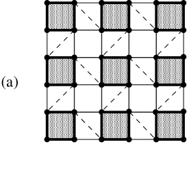
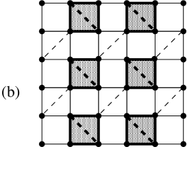
FIG. 2.: (a) The first plaquette structure (PE1): The bold solid, the thin solid and the dashed lines represent the coupling constants $J^{\prime}$, $\lambda J^{\prime}$ and $\lambda J$, respectively. (b) The second plaquette structure (PE2): The bold solid, bold dashed, the thin solid, and the thin dashed lines represent the coupling constants $J^{\prime}$, $J$, $\lambda J^{\prime}$ and $\lambda J$, respectively.

Instead of perturbing about isolated dimers, any set of disconnected units can be used. Using a plaquette basis allows the investigation of plaquette type order. Because each plaquette has 16 rather than 4 states it is not possible to derive series of the same length as with dimer expansions.

Following Koga and Kawakami[9], we have computed two kinds of plaquette expansions (PE1 and PE2), which respectively take the set of plaquettes without the diagonal $J$ bonds and the set with diagonal $J$ bonds as the unperturbed Hamiltonian. To make the expansion possible it is necessary to introduce an expansion parameter $\lambda\leq 1$ which modifies the interactions not included in $H_{0}$. This is illustrated in Figure 2. The series are then computed in powers of $\lambda$. The analysis evaluates these at $\lambda=1$, corresponding to the original Hamiltonian.

For PE1 we have computed series to order $\lambda^{8}$, $\lambda^{7}$, $\lambda^{6}$ for the ground state energy, triplet excitation energies $\Delta({\bf k})$ and staggered susceptibility $\chi_{\rm AF}$ respectively. This is one additional term for $E_{0}$ and two additional terms for $\Delta({\bf k})$ and $\chi_{\rm AF}$ over Ref. [9]. The calculation is computationally demanding, even with our efficient program. For example, the computation of $\Delta({\bf k})$ to order $\lambda^{7}$ took about 10 days and required 1.8GB memory on an SGI Origin 2400 system with a 400MHz R12000 CPU. The effort for each additional term requires factors of approximate 50 and 15 increase in CPU time and memory, respectively. For the second expansion (PE2) the series have been computed to order $\lambda^{7}$ for the ground state energy and the singlet excitation spectrum, and to order $\lambda^{6}$ for the triplet excitation $\Delta({\bf k})$ and staggered susceptibility $\chi_{\rm AF}$. In Tables I and II we present the series for the ground state energy, the triplet gap $\Delta$ at ${\bf k}=0$ and staggered susceptibility $\chi_{AF}$ for $J/J^{\prime}=1.25$ and 1.4. Other series are available on request. The analysis is left for the next Section.

C Columnar Dimer Expansions

FIG. 3.: Columnar dimerization pattern. The bold solid, the thin solid and the dashed lines represent the coupling constants $J^{\prime}$, $\lambda J^{\prime}$ and $\lambda J$, respectively.

A plausible candidate for the intermediate phase is the columnar dimer phase, as shown in Fig. 3. For both the spin-${1\over 2}$ $J_{1}-J_{2}$ Heisenberg model[17] and the spin-${1\over 2}$ Heisenberg model on an anisotropic triangular lattice[18], there appears to be a columnar dimer ordered phase adjacent to the Néel ordered phase. To make the expansion possible it is necessary to introduce an expansion parameter $\lambda\leq 1$ which modifies the interactions not included in $H_{0}$. This is illustrated in Figure 3. The series are then computed in powers of $\lambda$. The analysis evaluates these at $\lambda=1$, corresponding to the original Hamiltonian.

We have computed series to order $\lambda^{10}$, $\lambda^{9}$, $\lambda^{9}$ for the ground state energy, the antiferromagnetic susceptibility $\chi_{\rm AF}$, and the triplet excitation energies $\Delta({\bf k})$ respectively. This calculation involves 290215 linked clusters up to 10 sites. In Table I we present the series for the ground state energy $\chi_{AF}$ for $J/J^{\prime}=1.25$ and 1.4. Other series are available on request. The analysis is left for the next Section.

D Ising Expansions for Néel order

For small $J/J^{\prime}$, the model will have a Néel ordered phase with long range antiferromagnetic order (in the $z$ direction). To construct an Ising expansion, we introduce an exchange anisotropy parameter $\lambda$, and write the Hamiltonian as

$$H=H_{0}+\lambda V~{},$$ (9)

where

$$H_{0} = J\sum_{{\rm diag}}S_{i}^{z}S_{j}^{z}+J^{\prime}\sum_{{\rm axial}}S_{i}^{z}S_{j}^{z}~{},$$ (10)

$$V =J \sum_{{\rm diag}}(S_{i}^{x}S_{j}^{x}+S_{i}^{y}S_{j}^{y})+J^{\prime}\sum_{{\rm axial}}(S_{i}^{x}S_{j}^{x}+S_{i}^{y}S_{j}^{y})~{},$$ (11)

The unperturbed ground state is the classical Néel state with energy $E_{0}/N=-J^{\prime}/2+J/8$. The perturbation $V$ flips pairs of neighbouring spins. Series are developed in powers of $\lambda$ and evaluated at $\lambda=1$, which recovers the original Hamiltonian. We have obtained series for the ground state energy per site, $E_{0}/N$, and the staggered magnetization (order parameter) $M$ to order $\lambda^{12}$, extending our previous calculation by 3 terms. We have also computed a new series, to order $\lambda^{12}$ for the perpendicular susceptibility $\chi_{\perp}$. The resulting series for the ground state energy and the staggered magnetization (order parameter) $M$ for $J/J^{\prime}=1.25$ and 1.4 are listed in Tables I and III; the series for other values of $J/J^{\prime}$ are available on request. For details of the analysis we refer to our previous paper[8]. Results of the analysis are presented in the next section.

E Ising Expansions for Helical Order

As discussed by Albrecht and Mila[7], the classical system has planar helical order for $J/J^{\prime}>1$. Starting from a reference spin in the $z$ direction, each neighboring spin is rotated by an angle $q$, as shown in Figure 1. The twist is determined by minimization of the energy and yields

$$q=\cases{\pi,&$J\leq J^{\prime}$;\cr\arccos(-J^{\prime}/J),&$J>J^{\prime}$.\cr}$$ (12)

To develop an Ising expansion about such a helically ordered state we transform the Hamiltonian by rotating the spin axes at each site. The transformed Hamiltonian is

$$H=H_{1}+\lambda(H_{2}+H_{3}),$$ (13)

where

$$H_{1} = J\cos(2q)\sum_{\rm diag}S_{i}^{z}S_{n}^{z}+J^{\prime}\cos(q)\sum_{\rm axial}S_{i}^{z}S_{j}^{z}~{},$$ (14)

$$H_{2} = J\sum_{\rm diag}\left[S_{i}^{y}S_{n}^{y}+\cos(2q)S_{i}^{x}S_{n}^{x}+\sin(2q)(S_{i}^{z}S_{n}^{x}-S_{i}^{x}S_{n}^{z})\right]~{},$$ (15)

$$H_{3} = J^{\prime}\sum_{\rm axial}\left[S_{i}^{y}S_{j}^{y}+\cos(q)S_{i}^{x}S_{j}^{x}+\sin(q)(S_{i}^{z}S_{j}^{x}-S_{i}^{x}S_{j}^{z})\right]~{}.$$ (16)

and where exchange anisotropy is introduced through the perturbation parameter $\lambda$.

We have computed series for the ground state energy and the order parameter to order $\lambda^{12}$, for various choices of $q$ and the ratio $J/J^{\prime}$. The resulting series for the ground state energy and the staggered magnetization (order parameter) $M$ for $J/J^{\prime}=1.25$ and 1.4 are listed in Tables I and III; other series can be supplied on request. We are not aware of previous series of this type for this model.

III Results and Discussion

In this Section we present a variety of results obtained from analysis of the various series expansions. The analysis has been carried out using integrated first-order inhomogeneous differential approximants and Padé approximants[15] to extrapolate each series to the physical value $\lambda=1$.

FIG. 4.: The ground state energy versus $J/J^{\prime}$ obtained from the Néel ordered Ising expansion (N), columnar dimer expansion (C), plaquette expansion (P), and helical order Ising expansion (H). The energy of the exact dimer state is also presented (D).

A Ground State Energy

The nature of the ground state for any particular $J/J^{\prime}$ can be determined by comparing the energies of various candidate states. Our analysis shows that, among all the series expansions we have calculated, the ground state energy from the Ising expansion about Néel order has the lowest energy for coupling $J/J^{\prime}<1.45$, while the ground state energies obtained from the columnar dimer expansion and from the Néel order Ising expansion remain nearly equal through $J/J^{\prime}\gtrsim 1.2$. For example, we estimate the ground state energy at $J/J^{\prime}=1.25$ as

$$E_{0}/NJ^{\prime}=\cases{-0.5628(15),&N\'{e}el order;\cr-0.5586(10),&helical order;\cr-0.5599(3),&PE1;\cr-0.5584(8),&PE2;\cr-0.563(1),&columnar dimer.\cr}$$ (17)

and at $J/J^{\prime}=1.40$ as

$$E_{0}/NJ^{\prime}=\cases{-0.561(3),&N\'{e}el order;\cr-0.554(1),&helical order;\cr-0.5548(5),&PE1;\cr-0.5525(10),&PE2;\cr-0.557(2),&columnar dimer.\cr}$$ (18)

where we have used the classical-$q$ value in Eq. (12) in the calculation of helical order. In Table IV we show details of the analysis from the latter case $J/J^{\prime}=1.4$ for both the Ising expansion about Néel order and the plaquette expansion (PE1), from which we estimate the values in (18). The ground state energies obtained from various expansions versus $J/J^{\prime}$ are given in Fig. 4. Since the energy from the second plaquette expansion is slightly higher than that from the first plaquette expansion, we do not show the results of the second plaquette expansion. Our results are thus in disagreement with ref. [9], which claimed that the plaquette phase has the lowest energy. Of course these energies are all very close to each other and the estimated errors are subjective confidence limits. However inspection of the data in Table IV shows that the Ising expansion about Néel order consistently gives lower energy estimates.

Our results also argue against helical order being a stable ground state. In Figure 5 we show estimates of the ground state energy from Ising expansions about helical order, as a function of angle $q$, for the two coupling ratios $J/J^{\prime}=1.25$, 1.40. In each case the curve shows no indication of a minimum at some $q_{c}$, but rather decreases monotonically towards $q=\pi$, corresponding to Néel order.

FIG. 5.: The ground state energy versus $q$ for helical order.

Over the region $1.2\lesssim J/J^{\prime}\lesssim 1.45$, the ground state energies obtained from the Néel ordered Ising expansion and from the columnar dimer expansion have some overlap after considering the error bars, so they are both good candidates for the ground state of the Shastry-Sutherland model.

B Staggered Magnetization and Perpendicular Susceptibility

The staggered magnetization and perpendicular susceptibility will be non-zero in a phase with long range antiferromagnetic order, and are expected to vanish at a transition point to a magnetically disordered or spin-liquid phase. Effective Lagrangian theory predicts a relationship $\rho_{s}=v^{2}\chi_{\perp}$ where $\rho_{s}$ is the spin stiffness and $v$ the spin-wave velocity. In Figures 6 we show estimates of $M$ and $\chi_{\perp}$ versus $J/J^{\prime}$, from the Ising expansion about Néel order. It can be seen that both quantities behave similarly, decreasing from their values at $J=0$ and vanishing at around $J/J^{\prime}=1.2\pm 0.1$. The error bars are large and the vanishing point can not be obtained to high precision. However our new extended series shows a much sharper drop-off in $M$ than given in our previous work[8]. Thus it is possible that the true transition point is at or below 1.20.

For the Ising expansion about helical order the magnetization $M$ at $\lambda=1$ (for the classical $q$ value) is zero, within error bars, for all $J/J^{\prime}$. This strengthens our conclusion, from the ground state energy results, that a helical phase is not present.

FIG. 6.: The staggered magnetization $M$ and the perpendicular susceptibility $\chi_{\perp}$ versus $J/J^{\prime}$. The solid points with error bars are the estimates from the Ising expansion about Néel order.

C Energy gap and susceptibility in the plaquette expansion

The main argument of Koga and Kawakami[9] for the existence of a plaquette intermediate phase in the system is based on analysis of the triplet gap at ${\bf k}=0$ and the staggered susceptibility series. In their series analysis, they assumed that the minimum triplet gap is at ${\bf k}=0$, and the transition lies in the same universality class as the classical 3D Heisenberg model (i.e. critical exponents $\gamma\simeq 1.4$, $\nu\simeq 0.71$). Using standard Dlog Padé approximants, they found an apparent critical singularity at $\lambda>1$ for $J/J^{\prime}\geq 1.16$. This would imply a non-zero spin gap for $J/J^{\prime}\geq 1.16$ for the original Hamiltonian (1). The above assumption is valid for the transition to Néel order, but if there was an intermediate phase, the transition from the plaquette phase to this intermediate phase might not lie in the same universality class as the classical 3D Heisenberg model, and the minimum triplet gap might not be at ${\bf k}=0$. In the analysis with our longer series, we find indeed that the minimum triplet gap is not at ${\bf k}=0$ for $J/J^{\prime}\gtrsim 1.25$, and also that the transition does not lie in the classical 3D Heisenberg universality class.

FIG. 7.: The triplet dispersion for various $\lambda$ and $J/J^{\prime}=1.40$ along the line connecting ${\bf k}=(0,0)$ and ${\bf k}=(\pi/4,3\pi/16)$ obtained from the first plaquette expansion (PE1).

Firstly, let us discuss the first plaquette expansion (PE1). Here for $J/J^{\prime}\lesssim 1.25$, or for larger values of $J/J^{\prime}$ with small values of $\lambda$, we find the minimum triplet gap is at ${\bf k}=0$; but for $J/J^{\prime}\gtrsim 1.25$ and $\lambda\sim 1$, it is no longer at ${\bf k}=0$. For example for $J/J^{\prime}=1.40$, the dispersion for various $\lambda$ along the line connecting ${\bf k}=(0,0)$ and ${\bf k}=(\pi/4,3\pi/16)$ is shown in Fig. 7, where we can see that for $\lambda\lesssim 0.75$, the minimum gap is located at ${\bf k}=0$, while for larger $\lambda$, the minimum gap is located at about ${\bf k}=(\pi/4,3\pi/16)$, and the dispersion near the minimum is quite flat. The series for the triplet gap at ${\bf k}=(\pi/4,3\pi/16)$ is

$$\Delta(\pi/4,3\pi/16)/J^{\prime} =1-0.3077152787\lambda-0.2293662299\lambda^{2}-0.0346064996\lambda^{3}$$ (20)

$$-0.0741227651\lambda^{4}-0.0176489659\lambda^{5}-0.0400694385\lambda^{6}-0.0030161628\lambda^{7}+O(\lambda^{8})$$

Table V shows estimates of the critical point $\lambda_{c}$ and critical index from both the spin gap and susceptibility series for the coupling ratios $J/J^{\prime}=1.25$ and 1.40, using unbiased Dlog Padé approximants, where for $J/J^{\prime}=1.40$, we show the results for the spin gap at both ${\bf k}=0$ and ${\bf k}=(\pi/4,3\pi/16)$. Apart from the spin gap $\Delta(\pi/4,3\pi/16)$ at $J/J^{\prime}=1.40$, there is considerable scatter in the results, but several features are apparent. The spin gap series show decreasing estimates of $\lambda_{c}$ with increasing order for both $J/J^{\prime}$ ratios. The data are more consistent with the conclusion $\lambda_{c}\leq 1$, rather than $\lambda_{c}>1$. For the spin gap $\Delta(\pi/4,3\pi/16)$ at $J/J^{\prime}=1.40$, the unbiased Dlog Padé approximants give very convergent results, with the critical point $\lambda_{c}=0.988$ and critical index $\nu=0.43$. This indicates instability of the plaquette phase at $\lambda=1$, at least for this coupling ratio. This also indicates that there is indeed an intermediate phase. Note that the critical index $\nu$ obtained here is about the same as that obtained from the dimer series, suggesting that this transition might belong to the same new universality class. Our analysis shows that the transition probably does not belong in the classical 3D Heisenberg universality class for $J/J^{\prime}\gtrsim 1.1$. Because the critical index $\nu$ for the minimum gap is much smaller than 1, we have obtained the dispersion results shown in Fig. 7 by performing the series extrapolation in a new variable

$$\delta=1-(1-\lambda/\lambda_{c})^{\nu}~{}.$$ (21)

in order to take the singular behavior into account.

Finally we consider the second plaquette expansion (PE2). The minimum triplet gap is no longer at ${\bf k}=0$, at least for small to moderate $\lambda$. This can be seen from the first few terms of the series

$$\Delta(k_{x},k_{y})/J^{\prime}=1-{4\lambda\over 6}(\cos k_{x}+\cos k_{y})+{J\lambda\over 3J^{\prime}}\cos(k_{x}+k_{y})$$ (22)

which gives the minimum gap at $k_{x}=k_{y}=\arccos(J^{\prime}/J)$. It seems likely that the minimum triplet gap will remain at ${\bf k}\not=0$, even for $\lambda\simeq 1$, although the series in this region are too erratic to confirm this. For this choice of unperturbed Hamiltonian we are also able to compute the excitation spectrum for the singlet excitation and we have obtained series to order $\lambda^{7}$. The minimum singlet gap is at ${\bf k}=0$ and appears to be smaller than the triplet gap. An attempt to locate the critical point $\lambda_{c}$ by Dlog Padé approximants to this series was hampered by poor convergence. We have attempted other analysis procedures, but without great success. But since the ground state energy from the second plaquette expansion (PE2) is higher than that obtained from both the first plaquette expansion and the Néel ordered Ising expansion, the probability of having the second plaquette configuration as the intermediate phase is remote.

FIG. 8.: The triplet gap $\Delta({\bf k})/J^{\prime}$ versus $\lambda$ for ${\bf k}=(0,0)$, $(\pi,0)$ and $(0,\pi)$ and $J/J^{\prime}=0.875$, and 2. Several different integrated differential approximants to the series are shown.

D The energy gap in the columnar dimer expansion

Finally we discuss the triplet dispersion obtained from the columnar dimer expansion. Here for $J/J^{\prime}\lesssim 1.15$, we find the minimum gap is located at momentum ${\bf k}=(0,\pi)$, as expected, since we expect to have a transition to the Néel ordered phase for small $J/J^{\prime}$. Fig. 8 show the gap at ${\bf k}=(0,0)$, $(\pi,0)$ and $(0,\pi)$ for $J/J^{\prime}=0.875$ versus $\lambda$ obtained from the integrated differential approximants[15] to the series. We can see that the minimum gap vanishes at a critical value $\lambda_{c}<1$. We also expect this transition (to Neél order) to lie in the same universality class as the classical 3D Heisenberg model. To determine the phase boundary of columnar dimer order, we can use Dlog Padé approximants to both the series for the minimum gap and for the antiferromagnetic susceptibility. To get more reliable estimates for the critical point, we assume the critical exponents to be $\gamma\simeq 1.4$, $\nu\simeq 0.71$. The results are shown in the phase diagram Fig. 9, where we can see that $\lambda_{c}=0.514(6)$ for $J=0$, and that $\lambda_{c}$ increases for increasing $J$. For $J/J^{\prime}=1.15$, we estimate $\lambda_{c}=0.97(5)$, but unfortunately the biased Dlog Padé results here are not accurate enough to tell whether $\lambda_{c}$ is larger than 1.

For $J/J^{\prime}\gtrsim 1.75$, we find that the minimum gap is located at ${\bf k}=(0,0)$. Fig. 8 also shows the gap at ${\bf k}=(0,0)$, $(\pi,0)$ and $(0,\pi)$ for $J/J^{\prime}=2$ versus $\lambda$. Once again, one can locate the phase boundary by using the Dlog Padé approximants to the series for the minimum gap, and the results are also shown in Fig. 9. We see that as $J/J^{\prime}$ decreases, $\lambda_{c}$ increases, but again, the analysis is not accurate enough to tell whether $\lambda_{c}$ is larger than 1 in the intermediate region.

In the analysis, we also note that the gap at ${\bf k}=(\pi,0)$ shows some peculiar features, as shown in Fig. 8. For all values of $J/J^{\prime}$, the majority of integrated differential approximants to the series show that the gap increases for small $\lambda$, then decreases dramatically to zero for $\lambda\sim 0.5$. The majority of Dlog Padé approximants to the series also show that the series has a critical point at $\lambda\sim 0.5$ with very small critical index ($\sim 0.2$). But we believe this peculiar behavious is an artefact of the short series.

For the most interesting region $1.15\lesssim J/J^{\prime}\lesssim 1.75$, the situation is quite complicated: the location of the minimum gap depends on both $J/J^{\prime}$ and $\lambda$. We take the mid-point for the presumed intermediate phase, $J/J^{\prime}=4/3$, as example. For $\lambda$ near 1, we find the minimum gap for $J/J^{\prime}=4/3$ is at ${\bf k}=(0.47,2.80)$, slightly away from $(0,\pi)$. The standard Dlog Padé approximants to the series for the minimum gap gives a critical point $\lambda_{c}=1.0(1)$, with critical index $\nu\sim 0.4$. This seems to be consistent with the indices obtained from the dimer and plaquette expansions, Since the standard Dlog Padé approximants cannot tell whether $\lambda_{c}$ is larger than 1, we examine the extrapolations for the gap itself obtained from integrated differential approximants. The results for the gap at ${\bf k}=(0.47,2.80)$, $(0,0)$ and $(0,\pi)$ are shown in Fig. 10. The gap at $\lambda=1$ for ${\bf k}=(0.47,2.80)$ is very small ($\sim 0.1J^{\prime}$) when estimated from the direct $\lambda$-series. When analysed in term of variable $\delta$ (Eq. 21) the gap is compatible with zero. If the gap vanishes at or before $\lambda=1$, the columnar dimer phase would also be ruled out as intermediate phase for the Shastry-Sutherland model.

FIG. 9.: The phase diagram for columnar dimer order, where the curve in the small $J/(J+J^{\prime})$ region is determined by the Dlog Padé approximants to the gap at ${\bf k}=(0,\pi)$ and the antiferromagnetic susceptibility $\chi_{AF}$, and we assume the transition lies in at the same universality class as the classical 3D Heisenberg model. The curve in the large $J/(J+J^{\prime})$ region is determined by the Dlog Padé approximants to the gap at ${\bf k}=(0,0)$.

FIG. 10.: The triplet gap $\Delta({\bf k})/J^{\prime}$ versus $\lambda$ for ${\bf k}=(0,0)$, $(0.47,2.80)$ and $(0,\pi)$ and $J/J^{\prime}=4/3$. Several different integrated differential approximants to the series are shown.

IV Conclusions

We have attempted to further elucidate the nature of the phase diagram of the Shastry-Sutherland spin model at $T=0$, by series expansion methods. We have significantly extended previous series, computed by ourselves[8] and others[9], and we have also derived a number of new series. The analysis of the various series allows us to draw some fairly firm conclusions, as well as others which are more tentative.

The first question is whether an intermediate phase between the Néel-ordered phase and the dimer phase exists at all. It seems rather clear that the singlet dimer phase, with a simple singlet-product ground state, persists from large $J/J^{\prime}$ down to $J/J^{\prime}\simeq 1.5-1.6$. In our previous work[8] we argued that there is a direct first-order transition from the dimer phase to Néel order at this point. Our present results show the staggered magnetization and perpendicular susceptibility in the Néel phase vanishing at $J/J^{\prime}\simeq 1.2$, with large uncertainty $\pm 0.1$. This appears more consistent with the Néel phase terminating at a second-order phase transition, so that there may indeed be an intermediate phase stretching over a very small range of coupling constants $1.20\lesssim J/J^{\prime}\lesssim 1.5$, in agreement with the suggestion of Koga and Kawakami[9].

Carpentier and Balents[19] have recently discussed an effective mean-field theory approach to the generalized Shastry-Sutherland model. They argue that a direct continuous transition from the Néel phase to the dimer phase is not possible. If this argument is accepted, it means that the vanishing of the order parameter and susceptibility in the Néel phase cannot be associated with a second order transition directly to the dimer phase. It follows that an intermediate phase must exist, over at least a small range of couplings.

The next question is the nature of the transitions from the Néel and dimer phases, respectively, into the intermediate phase. The vanishing staggered magnetization and perpendicular susceptibility in the Néel phase indicate a 2nd order transition; but we are unable to estimate the critical exponents, since we do not have explicit series coefficients for an expansion in $J/J^{\prime}$. The vanishing energy gap would indicate that the transition from the dimer phase is also 2nd order; but the result of Knetter et al.[11] showing that the two-particle bound-state energy vanishes before the single triplet gap indicates that more work needs to be done to characterize this transition also. It is interesting that one-particle gaps appears to vanish with a similar exponent in the dimer expansion, the plaquette expansion, and also the columnar dimer expansion.

A further question concerns the nature of the intermediate phase. None of the suggested phases exhibit a ground-state energy which is distinctly lower than the Néel energy in the relevant coupling regime. Our results do not support the suggestion[9] that the intermediate phase is plaquette ordered. The extrapolated ground-state energy from the Néel expansion consistently lies below that from the plaquette expansion; and the triplet gap from the plaquette expansion appears to vanish at or before the physical value $\lambda=1$ is reached, indicating instability in this phase. Our longer series thus appear to contradict the conclusions of Koga and Kawakami[9]. Equally, our results do not support the suggestion that the intermediate phase is helically ordered[7, 10]. The extrapolated ground-state energy from the Néel expansion consistently lies below that of the helically-ordered state, for any value of the spin orientation $q$ other than $\pi$. We note that the mean-field approach of Albrecht and Mila[7] is strictly only valid for $d>2$; while the $1/N$ expansion approach of Chung, Marston, and Sachdev[10] is of doubtful validity for the spin-$\frac{1}{/}2$ case, and is certainly not quantitatively accurate.

We have also explored the possibility that the intermediate phase is a columnar dimer phase, as in the $J_{1}-J_{2}$ Heisenberg model[17], or the spin-${1\over 2}$ Heisenberg model on an anisotropic triangular lattice[18]. The extrapolated ground state energy for this state is comparable with that of the Néel state, within error bars, and the triplet gap from this expansion shows a window $1.15\lesssim J/J^{\prime}\lesssim 1.5$ in which it may remain finite, though very small, at the physical value $\lambda=1$. This remains a possible candidate for the intermediate phase, although our data are not sufficiently accurate to allow a definitive conclusion.

The nature of an intermediate state in this model thus remains an open question. It could, for example, be a structureless spin liquid, in which case a signature of this phase is elusive. Carpentier and Balents[19] have also discussed possible intermediate phases in the generalized model, including a WISDQ (weakly incommensurate spin-density wave) ordered state -i.e. a periodic modulation of the expectation value of the total spin on each dimer - and a ‘fractionalized’ state, with topological order and deconfined spin-$\frac{1}{/}2$ excitations (‘spinons’). We currently have no information to offer regarding these states. The fact that the energy gap drops to zero before or near the physical value $\lambda=1$ in every expansion we have tried appears to suggest that the intermediate phase is gapless, or near to it. Further support for this idea is given by the strong finite-size dependence of the exact diagonalization results of Miyahara and Ueda[5] in this region.

The material SrCu₂(BO₃)₂ appears to lie within the dimer phase of the Shastry-Sutherland model. Original estimates $J/J^{\prime}=1.47$[5, 8] put the material close to the phase transition point, and it was argued that some of the unusual properties of the material were due to this closeness. A more recent estimate[11], including interactions in the third direction, gives $J/J^{\prime}\simeq 1.66$, somewhat beyond even the point at which the two-particle gap vanishes. This puts the material clearly within the dimer phase and hence the question of intermediate phases is primarily of theoretical interest.

It is clear that much work remains to be done on this fascinating model. It would be interesting to confirm and extend the results of Knetter et al.[11] concerning the transition from the dimer phase; and also to try and construct series coefficients for an expansion in $J/J^{\prime}$ in the Néel phase. New numerical methods are badly needed to explore the intermediate phase also: the best nmethod to employ here remains a puzzle.

TABLE I.: Series coefficients for the ground-state energy per site $E_{0}/(NJ^{\prime})$ obtained from the Ising expansion about Néel-order (Néel), the helical-order (helical) expansion, the columnar dimer expansion, and from the plaquette expansion without diagonal bonds (PE1), and with diagonal bonds (PE2) for $J/J^{\prime}=1.25,1.4$. Series coefficients of $\lambda^{i}$ are listed.

$i$	PE1	PE2	Helical	Néel	columnar dimer
	$J/J^{\prime}=1.25$
0	-5.000000000000$\times 10^{-1}$	-4.218750000000$\times 10^{-1}$	-3.562500000000$\times 10^{-1}$	-3.437500000000$\times 10^{-1}$	-3.750000000000$\times 10^{-1}$
1	0.000000000000	0.000000000000	0.000000000000	0.000000000000	0.000000000000
2	-3.575303819444$\times 10^{-2}$	-1.577687449269$\times 10^{-1}$	-2.054711318598$\times 10^{-1}$	-2.857142857143$\times 10^{-1}$	-1.904296875000$\times 10^{-1}$
3	-9.498878761574$\times 10^{-3}$	2.403841825921$\times 10^{-2}$	4.163537328971$\times 10^{-2}$	1.020408163265$\times 10^{-1}$	7.141113281250$\times 10^{-3}$
4	-6.520377148279$\times 10^{-3}$	-2.785619169517$\times 10^{-3}$	-4.669142343282$\times 10^{-2}$	-9.273368951135$\times 10^{-2}$	9.905815124512$\times 10^{-3}$
5	-3.110192567684$\times 10^{-3}$	1.333554456619$\times 10^{-3}$	2.832044653274$\times 10^{-2}$	1.575551772772$\times 10^{-1}$	-9.499887625376$\times 10^{-3}$
6	-2.051453756690$\times 10^{-3}$	-9.330263748650$\times 10^{-3}$	-3.363486912444$\times 10^{-2}$	-2.473894356829$\times 10^{-1}$	-1.780716847214$\times 10^{-2}$
7	-1.134481706160$\times 10^{-3}$	9.793071057074$\times 10^{-3}$	3.693336765114$\times 10^{-2}$	4.097681140990$\times 10^{-1}$	1.494069254463$\times 10^{-2}$
8	-7.196107350240$\times 10^{-4}$		-5.318671447970$\times 10^{-2}$	-8.162334082025$\times 10^{-1}$	-3.803820899197$\times 10^{-4}$
9			7.567434418701$\times 10^{-2}$	1.693646904376	9.729690462284$\times 10^{-4}$
10			-1.138657557136$\times 10^{-1}$	-3.494392524807	-2.666137442909$\times 10^{-3}$
11			1.726680824433$\times 10^{-1}$	7.456679516027
12				-1.646408487950$\times 10^{1}$
	$J/J^{\prime}=1.40$
0	-5.000000000000$\times 10^{-1}$	-4.125000000000$\times 10^{-1}$	-3.535714285714$\times 10^{-1}$	-3.250000000000$\times 10^{-1}$	-3.750000000000$\times 10^{-1}$
1	0.000000000000	0.000000000000	0.000000000000	0.000000000000	0.000000000000
2	-3.392361111111$\times 10^{-2}$	-1.678565705128$\times 10^{-1}$	-1.943166023166$\times 10^{-1}$	-3.125000000000$\times 10^{-1}$	-1.950000000000$\times 10^{-1}$
3	-8.058449074074$\times 10^{-3}$	2.952951931067$\times 10^{-2}$	3.629865386622$\times 10^{-2}$	1.367187500000$\times 10^{-1}$	1.659375000000$\times 10^{-2}$
4	-5.431377864048$\times 10^{-3}$	-1.145691038736$\times 10^{-3}$	-4.218721381575$\times 10^{-2}$	-1.664227322346$\times 10^{-1}$	1.704765625000$\times 10^{-2}$
5	-2.536510876037$\times 10^{-3}$	2.724731917375$\times 10^{-3}$	2.276170842636$\times 10^{-2}$	3.302972722063$\times 10^{-1}$	-1.338582682292$\times 10^{-2}$
6	-1.754982806912$\times 10^{-3}$	-1.315792108890$\times 10^{-2}$	-3.202093475641$\times 10^{-2}$	-6.320111458811$\times 10^{-1}$	-1.870258387587$\times 10^{-2}$
7	-1.017310795905$\times 10^{-3}$	1.282279331689$\times 10^{-2}$	2.995390698796$\times 10^{-2}$	1.313875979565	1.669764147147$\times 10^{-2}$
8	-7.033788209007$\times 10^{-4}$		-4.311390066885$\times 10^{-2}$	-3.190631154651	-1.134220766188$\times 10^{-3}$
9			5.834414925135$\times 10^{-2}$	8.019181935184	-6.547755059723$\times 10^{-3}$
10			-8.797286992572$\times 10^{-2}$	-2.044153224739$\times 10^{1}$	-1.637369775362$\times 10^{-3}$
11			1.341535224738$\times 10^{-1}$	5.383666306276$\times 10^{1}$
12				-1.457331428464$\times 10^{2}$

TABLE II.: Series coefficients for the triplet gap $\Delta/J^{\prime}$ at ${\bf k}=0$ and staggered susceptibility $\chi_{AF}$ obtained from the plaquette expansion without diagonal bonds (PE1), and with diagonal bonds (PE2) for $J/J^{\prime}=1.25,1.4$. Series coefficients of $\lambda^{i}$ are listed.

	PE1		PE2
$i$	$J/J^{\prime}=1.25$	$J/J^{\prime}=1.4$	$J/J^{\prime}=1.25$	$J/J^{\prime}=1.4$
triplet gap $\Delta/J^{\prime}$ at ${\bf k}=0$
0	1.000000000000	1.000000000000	1.000000000000	1.000000000000
1	-5.000000000000$\times 10^{-1}$	-4.000000000000$\times 10^{-1}$	-9.166666666667$\times 10^{-1}$	-8.666666666667$\times 10^{-1}$
2	-1.949508101852$\times 10^{-1}$	-1.558796296296$\times 10^{-1}$	5.848101551222$\times 10^{-4}$	-1.753739316239$\times 10^{-2}$
3	-1.215547789271$\times 10^{-2}$	6.279063786008$\times 10^{-3}$	3.919269654832$\times 10^{-1}$	7.809106177672$\times 10^{-1}$
4	-4.262073088443$\times 10^{-2}$	-3.063595079003$\times 10^{-2}$	-1.209759818705	-2.966617086045
5	-1.169575496893$\times 10^{-2}$	-4.837854449338$\times 10^{-3}$	2.808227188528	1.165893864520$\times 10^{1}$
6	-2.087090156347$\times 10^{-2}$	-1.752776610250$\times 10^{-2}$	-7.118402535782	-5.396727727606$\times 10^{1}$
7	-9.640627326157$\times 10^{-3}$	-8.067626260181$\times 10^{-3}$
staggered susceptibility $\chi_{AF}$
0	1.333333333333	1.333333333333	1.333333333333	1.333333333333
1	1.333333333333	1.066666666667	2.444444444444	2.311111111111
2	1.250353652263	7.572093621399$\times 10^{-1}$	2.323016302459	1.684709846149
3	1.201753927683	5.539876821845$\times 10^{-1}$	2.280972931735	1.010069843149
4	1.113460517630	3.809246267771$\times 10^{-1}$	2.075318140109	3.056543491121$\times 10^{-1}$
5	1.044513939707	2.747370398592$\times 10^{-1}$	2.415891359693	6.618315713507$\times 10^{-1}$
6	9.707650534281$\times 10^{-1}$	1.964730571491$\times 10^{-1}$	2.233378054361	4.157664670338$\times 10^{-1}$

TABLE III.: Series coefficients for the staggered magnetization $M$ obtained from the Ising expansion about Néel-order (Néel), and the helical-order (helical) expansion for $J/J^{\prime}=1.25,1.4$. Series coefficients of $\lambda^{i}$ are listed.

	helical		Néel
$i$	$J/J^{\prime}=1.25$	$J/J^{\prime}=1.4$	$J/J^{\prime}=1.25$	$J/J^{\prime}=1.4$
0	5.000000000000$\times 10^{-1}$	5.000000000000$\times 10^{-1}$	5.000000000000$\times 10^{-1}$	5.000000000000$\times 10^{-1}$
1	0.000000000000	0.000000000000	0.000000000000	0.000000000000
2	-1.976862628853$\times 10^{-1}$	-1.787535427319$\times 10^{-1}$	-3.265306122449$\times 10^{-1}$	-3.906250000000$\times 10^{-1}$
3	8.015745892489$\times 10^{-2}$	6.696385209168$\times 10^{-2}$	2.332361516035$\times 10^{-1}$	3.417968750000$\times 10^{-1}$
4	-2.020938451061$\times 10^{-1}$	-1.703648728139$\times 10^{-1}$	-6.249672540570$\times 10^{-1}$	-1.188130158850
5	1.595089057636$\times 10^{-1}$	1.186622673353$\times 10^{-1}$	1.247039703760	2.891792139388
6	-2.856270160505$\times 10^{-1}$	-2.387988493110$\times 10^{-1}$	-2.564444941065	-7.392698990572
7	3.509646624490$\times 10^{-1}$	2.550333854825$\times 10^{-1}$	5.414869562182	1.960927054837$\times 10^{1}$
8	-6.159923626864$\times 10^{-1}$	-4.541054989763$\times 10^{-1}$	-1.300042701432$\times 10^{1}$	-5.777973112981$\times 10^{1}$
9	9.506010225594$\times 10^{-1}$	6.635675648444$\times 10^{-1}$	3.100311343644$\times 10^{1}$	1.688382921512$\times 10^{2}$
10	-1.636489163183	-1.143031741464	-7.335660790958$\times 10^{1}$	-4.957990614738$\times 10^{2}$
11	2.726180882130	1.887668026020	1.769340004349$\times 10^{2}$	1.478774628135$\times 10^{3}$
12			-4.347120802018$\times 10^{2}$	-4.471290404091$\times 10^{3}$

TABLE IV.: The results of $\{m/n/l\}$ integrated differential approximants to the series for the ground state $E_{0}/NJ^{\prime}$ for $J/J^{\prime}=1.4$ from the Néel ordered Ising expansion and the plaquette expansion without diagonal bonds (PE1). An asterisk denotes a defective approximant.

n	$\{(n-3)/n/l\}$	$\{(n-2)/n/l\}$	$\{(n-1)/n/l\}$	$\{n/n/l\}$	$\{(n+1)/n/l\}$	$\{(n+2)/n/l\}$	$\{(n+3)/n/l\}$
Néel ordered Ising expansion
$l=0$
n= 3		-0.52170	-0.55795	-0.54979	-0.57974	-0.55498	-0.57207
n= 4	*	-0.55178	-0.55573	-0.56195	-0.56468	-0.56026	-0.55991
n= 5	-0.56212	-0.57002	-0.56907	-0.56264	-0.55989
n= 6	-0.56912	*	-0.56121
n= 7	-0.56405
$l=1$
n= 3		-0.55300	-0.55127	-0.55765	-0.57441	-0.56242	-0.55104
n= 4	-0.55139	*	-0.55545	-0.56380	*	-0.56002
n= 5	-0.56139	-0.56960	-0.56066	-0.56100
n= 6	-0.56503	-0.56097
$l=2$
n= 2		-0.56352	*	-0.55148	-0.55131	-0.60526	-0.57327
n= 3	-0.55123	-0.55086	-0.55252	*	-0.56628	-0.54598	-0.55427
n= 4	-0.55270	*	-0.55923	-0.55915	*
n= 5	-0.56600	-0.55917	-0.56079
n= 6	-0.56213
$l=3$
n= 1			-0.56410	-0.55914	-0.55010	-0.56012	-0.57599
n= 2		-0.56089	*	-0.55363	*	-0.56992	*
n= 3	-0.55104	-0.55440	-0.55944	-0.55918	-0.56186	-0.56198
n= 4	*	-0.55918	-0.55923	-0.56196
n= 5	-0.56143	-0.56258
plaquette expansion without diagonal bond (PE1)
$l=0$
n= 1					-0.55534	-0.55281	-0.55647
n= 2			-0.55246	-0.55301	-0.55390	-0.55473	-0.55482
n= 3		-0.55297	*	-0.55492	-0.55484
n= 4	-0.55425	-0.55448	-0.55484
n= 5	*
$l=1$
n= 1				*	-0.55243	*	-0.55344
n= 2			-0.55316	-0.55574	-0.55595	-0.55499
n= 3		*	-0.55587	-0.55467
n= 4	-0.55458	-0.55513
$l=2$
n= 1			*	-0.55270	*	*	*
n= 2		-0.55347	-0.55481	*	-0.55488
n= 3	*	-0.55496	-0.55487
n= 4	-0.55492

TABLE V.: $[n/m]$ Dlog Padé approximants to the series for the triplet gap $\Delta({\bf k})$ and antiferromagnetic susceptibility $\chi_{AF}$ for the plaquette expansion without diagonal bonds (PE1). An asterisk denotes a defective approximant.

n	$[(n-2)/n]$	$[(n-1)/n]$	$[n/n]$	$[(n+1)/n]$	$[(n+2)/n]$
	pole (residue)	pole (residue)	pole (residue)	pole (residue)	pole (residue)
$\Delta(0,0)$ for $J/J^{\prime}=1.25$
n= 1			1.4098(1.2718)	0.8592(0.2879)	1.2001(1.0957)
n= 2		1.0804(0.6523)	1.0530(0.6018)	1.0305(0.5502)	1.0181(0.5170)
n= 3	1.0555(0.6075)	0.9247(0.2175)∗	1.0074(0.4801)
n= 4	1.0089(0.4855)
$\Delta(0,0)$ for $J/J^{\prime}=1.4$
n= 1			2.0315(1.9470)	0.8107(0.1237)	1.5546(1.6732)
n= 2		1.2949(0.6512)	1.2016(0.5172)	1.1075(0.3712)	1.0273(0.2532)
n= 3	1.2181(0.5462)	0.7442(0.0227)∗	0.9352(0.1267)
n= 4	0.9454(0.1386)
$\Delta(\pi/4,3\pi/16)$ for $J/J^{\prime}=1.4$
n= 1			1.6055(1.4266)	0.638(0.0896)	1.4385(2.3132)
n= 2	$*$	0.9883(0.4300)	0.9889(0.4307)	0.985(0.4240)	1.0203(0.5055)
n= 3	0.9889(0.4307)	0.9884(0.4301)	0.9885(0.4302)
n= 4	0.9885(0.4302)
$\chi_{AF}$ for $J/J^{\prime}=1.25$
n= 1			0.9830(-0.8461)	1.2245(-1.6351)	0.9962(-0.7165)
n= 2	1.0003(-0.8898)	1.0739(-1.0477)	1.1011(-1.1273)	1.0825(-1.0510)
n= 3	1.1033(-1.1367)	1.0910(-1.0902)