Short-Range Correlations in ⁴He Liquid and Small ⁴He Droplets
described by the Unitary Correlation Operator Method

Abstract

The Unitary Correlation Operator Method (UCOM) is employed to treat short-range correlations in both, homogeneous liquid and small droplets of bosonic ⁴He atoms. The dominating short-range correlations in these systems are described by an unitary transformation in the two-body relative coordinate, applied either to the many-body state or to the Hamiltonian and other operators. It is shown that the two-body correlated interaction can describe the binding energy of clusters of up to 6 atoms very well, the numerical effort consisting only in calculating one two-body matrix element with Gaussian single-particle states. The increasing density of bigger droplets requires the inclusion of correlation effects beyond the two-body order, which are successfully implemented by a density-dependent two-body correlator. With only one adjusted parameter the binding energies and radii of larger droplets and the equation of state of the homogeneous ⁴He liquid can be described quantitatively in a physically intuitive and numerically simple way.

I Introduction

The quantum-mechanical description of ground state properties of interacting many-body systems is a long-standing challenge in theoretical physics. In general the problem is two-fold: The first task is to specify the interaction between the constituents in terms of a two-body potential. The second is to solve the quantum-mechanical many-body problem with that interaction.

For many-body systems composed of Helium atoms the first task, the construction of an appropriate interatomic potential, is solved rather precisely. The HFDHE2 potential of Aziz et al. AzNa79 is able to reproduce experimental transport coefficients in a wide temperature range. A simpler and less precise description of the interaction is given by the Lennard-Jones potential BoMi38 ; BeKe81

$$v(r)=4\epsilon\;[(\sigma/r)^{12}-(\sigma/r)^{6}]$$ (1)

with $\epsilon=10.22\text{K}$ and $\sigma=2.556\text{\AA}$. Since the emphasis of the investigations presented in this paper is more on novel concepts, which remarkably simplify the treatment of the many-body problem, we will restrict ourselves to this simple and widely used parameterization.

A common property of many realistic microscopic interactions — like van der Waals type potentials between neutral atoms or the nucleon-nucleon interaction in atomic nuclei — is a strong short-range repulsion, which induces strong short-range correlations in the quantum many-body state. The repulsive core prevents the particles to approach each other closer than the radius of this core such that the two-body density matrix is strongly depleted for particle distances smaller than the core radius. This effect cannot be described in a mean-field like picture or in terms of a superposition of a finite number of symmetrized product states.

In this work we treat these correlations with the Unitary Correlation Operator Method (UCOM), that has already been applied successfully in the framework of the nuclear many-body problem UCOM98 .

In the following section we introduce the general formalism of the Unitary Correlation Operator Method and derive analytic expressions for correlated wave functions and the correlated Hamiltonian. In the third section we determine the optimal correlation operator for liquid ⁴He from the two-body system and discuss the structure of the effective interaction generated by the unitary transformation. In section IV we investigate the homogeneous ⁴He liquid with that correlator and introduce a density-dependent two-body correlator that describes very well the influence of three- and more-body correlations. Finally, we successfully apply the density-dependent correlator to describe the ground state of small ⁴He droplets. Considering the great numerical simplification — only a few one-dimensional integrals have to be calculated — compared to Monte-Carlo-type calculations KaLe81 ; ScSc65 , the agreement of the results is excellent.

II Unitary Correlation Operator Method (UCOM)

II.1 Concept

The goal of the Unitary Correlation Operator Method (UCOM) is to describe short-range interaction-induced correlations by a unitary transformation of an uncorrelated many-body state with $N$ particles. The unitary operator $\bm{C}$ associated with this transformation can be written as an exponential of a hermitian generator $\bm{G}$

$$\bm{C}=\exp[-\mathrm{i}\,\bm{G}].$$ (2)

The generator is chosen to be an irreducible two-body operator

$$\bm{G}=\sum_{i<j}^{N}\bm{g}_{ij},$$ (3)

which describes genuine two-body correlations only. In principle we could add a three-body part to account for genuine three-body correlations. For the moment we omit this step to develop the basic formalism on a simple level.

The particular structure of the unitary transformation — which should reflect the properties of the short-range correlations — is described by the two-body generator $\bm{g}$. The repulsive core of the interaction leads to a suppression of the probability density within the range $r_{\text{core}}$ of the core. Uncorrelated many-body states that are symmetrized products of single-particle states lead, however, to a two-body density that does not show any depletion for relative distances $r<r_{\text{core}}$ between the pair of particles. Therefore the unitary transformation should shift those particles that are in the forbidden region of the repulsion to larger distances. This is done by means of a distance-dependent radial shift in the relative coordinate of two-particles. The hermitian generator of this shift in two-body space reads

$$\bm{g}=\frac{1}{2}\big{[}s(\bm{r})\;(\hat{\bm{r}}\cdot\vec{\bm{q}})+(\vec{\bm{q}}\cdot\hat{\bm{r}})\;s(\bm{r})\big{]},$$ (4)

where $\vec{\bm{q}}=\frac{1}{2}(\vec{\bm{p}}_{1}-\vec{\bm{p}}_{2})$ is the operator of the relative momentum, $\vec{\bm{r}}=\vec{\bm{x}}_{1}-\vec{\bm{x}}_{2}$ is the relative coordinate, and $\hat{\bm{r}}$ is the associated unit vector. The function $s(r)$ describes the size of the shift as function of the distance of the particles.

II.2 Correlated Wave Functions

First we want to apply the unitary correlation operator $\bm{C}$ to an uncorrelated many-body state $\,\big{|}{\Psi}\big{>}$ out of a low-momentum model space. The correlated many-body state $\,\big{|}{\tilde{\Psi}}\big{>}$ is defined by

$$\,\big{|}{\tilde{\Psi}}\big{>}=\bm{C}\,\big{|}{\Psi}\big{>}.$$ (5)

Here and in the following all correlated quantities are marked by a tilde.

In order to demonstrate the generic effect of the correlation operator we discuss first a two-body system with an uncorrelated two-body state $\,\big{|}{\psi}\big{>}$. Using the definition of the correlation operator $\bm{C}$ and the generator $\bm{g}$ (4) we can evaluate the correlated two-body wave function in coordinate representation explicitly UCOM98

$$\big{<}{\vec{X},\vec{r}}\big{|}\,{\bm{C}\,}\,\big{|}{\psi}\big{>}=\mathcal{R}_{-}(r)\;\big{<}{\vec{X},R_{-}(r)\,\hat{r}}\big{|}{\psi}\big{>}.$$ (6)

The respective transformation with the hermitian adjoint correlation operator ${{\bm{C}}}^{{\dagger}}$ leads to

$$\big{<}{\vec{X},\vec{r}}\big{|}\,{{{\bm{C}}}^{{\dagger}}\!}\,\big{|}{\psi}\big{>}=\mathcal{R}_{+}(r)\;\big{<}{\vec{X},R_{+}(r)\,\hat{r}}\big{|}{\psi}\big{>}.$$ (7)

The correlation operator acts in the relative coordinate $\vec{r}$ of the two-body system only, the center of mass coordinate $\vec{X}=\frac{1}{2}(\vec{x}_{1}+\vec{x}_{2})$ is invariant. According to the construction of the the generator (4) the unitary transformation corresponds to a radial shift in the relative two-body coordinate

$$\vec{r}\;\overset{\bm{C}}{\longmapsto}\;R_{-}(r)\,\hat{r}\;,\qquad\vec{r}\;\overset{{{\bm{C}}}^{{\dagger}}}{\longmapsto}\;R_{+}(r)\,\hat{r}.$$ (8)

The transformed relative distances are given by the correlation functions $R_{-}(r)$ and $R_{+}(r)$, respectively. Due the unitarity of the correlation operator $\bm{C}{{\bm{C}}}^{{\dagger}}=\bm{1}$ the correlation functions $R_{-}(r)$ and $R_{+}(r)$ are inverse to each other

$$R_{\pm}[R_{\mp}(r)]=r.$$ (9)

The conservation of the norm of the correlated two-body wave function is guaranteed by the metric factor $\mathcal{R}_{\pm}(r)$ in (6) and (7)

$$\mathcal{R}_{\pm}(r)=\frac{R_{\pm}(r)}{r}\sqrt{R_{\pm}^{\prime}(r)},$$ (10)

where $R_{\pm}^{\prime}(r)$ denotes the derivative of $R_{\pm}(r)$. It corresponds to the square root of the Jacobi determinant associated with the transformation of the normalization integral.

The correlation functions $R_{\pm}(r)$ that describe the coordinate transformation are connected to the function $s(r)$, which enters in the generator (4), by the integral equation

$$\pm 1=\int_{r}^{R_{\pm}(r)}\!\!\frac{\mathrm{d}\xi}{s(\xi)}.$$ (11)

For small shift distances the approximate relation

$$R_{\pm}(r)\approx r\pm s(r)$$ (12)

holds.

Since all correlated quantities can be expressed directly in terms of the correlation functions $R_{-}(r)$ and $R_{+}(r)$ we will use one of these as basic quantity to describe the detailed structure of the short-range correlations. The shift function $s(r)$ is only used for formal considerations and never specified explicitly.

II.3 Correlated Operators

Complementary to the definition of a correlated state (5) we can use the correlation operator to define correlated operators. For an arbitrary observable $\bm{O}$ the correlated operator $\tilde{\bm{O}}$ is given by the similarity transformation

$$\tilde{\bm{O}}={{\bm{C}}}^{{\dagger}}\bm{O}\,\bm{C}.$$ (13)

It is evident that the formulations in terms of correlated states and correlated operators are equivalent when expectation values or matrix elements are calculated

$$\big{<}{\tilde{\Psi}}\big{|}\,{\bm{O}}\,\big{|}{\tilde{\Psi}^{\prime}}\big{>}=\big{<}{\Psi}\big{|}\,{{{\bm{C}}}^{{\dagger}}\bm{O}\,\bm{C}}\,\big{|}{\Psi^{\prime}}\big{>}=\big{<}{\Psi}\big{|}\,{\tilde{\bm{O}}}\,\big{|}{\Psi^{\prime}}\big{>}.$$ (14)

Thus we can choose the formulation that is technically or intuitively better suited for the specific application under consideration. In most cases the formulation in terms of correlated operators is easier to apply in the many-body system. Moreover it provides a systematic approximation scheme that will be discussed in section II.4.

As for the correlated wave function we first discuss specific correlated operators for a two-body system. The generalization to many-body systems will be done in the following sections.

II.3.1 Correlated Two-Body Potential

The simplest operator of interest is the local two-body potential $v(\bm{r})$ that depends on the relative distance $\bm{r}$ only. To evaluate the correlated potential we use the results on the correlated two-body wave function to determine a general two-body matrix element of the form

$$\begin{split}&\big{<}{\psi}\big{|}\,{{{\bm{C}}}^{{\dagger}}v(\bm{r})\bm{C}}\,\big{|}{\psi^{\prime}}\big{>}\\[1.0pt] &\quad=\int\!\!\mathrm{d}^{3}r\,\mathrm{d}^{3}\!X\;\big{<}{\psi}\big{|}\,{{{\bm{C}}}^{{\dagger}}}\,\big{|}{\vec{X},\vec{r}}\big{>}\,v(r)\,\big{<}{\vec{X},\vec{r}}\big{|}\,{\bm{C}}\,\big{|}{\psi^{\prime}}\big{>}\\[-2.0pt] &\quad=\int\!\!\mathrm{d}^{3}r\,\mathrm{d}^{3}\!X\;\big{<}{\psi}\big{|}{\vec{X},\vec{r}}\big{>}\;v[R_{+}(r)]\;\big{<}{\vec{X},\vec{r}}\big{|}{\psi^{\prime}}\big{>}\\[2.0pt] &\quad=\big{<}{\psi}\big{|}\,{v[R_{+}(\bm{r})]}\,\big{|}{\psi^{\prime}}\big{>}.\end{split}$$ (15)

In going from the second to the third line we use equations (6) and (9) and substitute the integration variable $\vec{r}$ by $R_{-}(r)\,\hat{r}$. Since the two-body states are arbitrary this relation is valid on the operator level

$$\tilde{v}(\bm{r})={{\bm{C}}}^{{\dagger}}v(\bm{r})\bm{C}=v[R_{+}(\bm{r})].$$ (16)

Thus the correlated two-body potential $\tilde{v}(r)$ is given by the original potential with transformed radial coordinate $r\mapsto R_{+}(r)$.

II.3.2 Correlated Kinetic Energy

The correlated operator of the kinetic energy in the two-body system is slightly more complicated due to its momentum dependence. First we decompose the operator of the two-body kinetic energy $\bm{T}_{2}$ in a center of mass contribution $\bm{t}_{\mathrm{cm}}$ and an relative part $\bm{t}_{\mathrm{rel}}$

$$\bm{T}_{2}=\bm{t}_{\mathrm{cm}}+\bm{t}_{\mathrm{rel}}=\frac{1}{2M}\vec{\bm{P}}^{2}+\frac{1}{2\mu}\vec{\bm{q}}^{2}.$$ (17)

The operator of the center of mass momentum $\vec{\bm{P}}=\vec{\bm{p}}_{1}+\vec{\bm{p}}_{2}$ commutes with the correlation operator, i.e., the operator of the center of mass kinetic energy is invariant under the unitary transformation. The correlation operator acts on the relative part $\bm{t}_{\mathrm{rel}}$ of the kinetic energy only. A similar calculation as for the local potential leads to the following structure of the correlated relative kinetic energy UCOM98

$$\tilde{\bm{t}}_{\mathrm{rel}}={{\bm{C}}}^{{\dagger}}\bm{t}_{\mathrm{rel}}\,\bm{C}=\bm{t}_{\mathrm{rel}}+\tilde{\bm{t}}_{\Omega}+\tilde{\bm{t}}_{r}+\tilde{u}(\bm{r}).$$ (18)

Besides $\bm{t}_{\mathrm{rel}}$ an additional momentum dependent term appears in the correlated relative kinetic energy, which can be formulated in terms of a tensorial effective mass correction. It is conveniently split into a correction for the radial part $\tilde{\bm{t}}_{r}$ and a different correction for the angular component $\tilde{\bm{t}}_{\Omega}$

$$\tilde{\bm{t}}_{\Omega}=\frac{1}{2\tilde{\mu}_{\Omega}(\bm{r})}\,\frac{\vec{\bm{l}}^{2}}{\bm{r}^{2}}\;,\qquad\tilde{\bm{t}}_{r}=(\vec{\bm{q}}\cdot\hat{\bm{r}})\frac{1}{2\tilde{\mu}_{r}(\bm{r})}(\hat{\bm{r}}\cdot\vec{\bm{q}}),$$ (19)

where $\vec{\bm{l}}=\vec{\bm{r}}\times\vec{\bm{q}}$ is the operator of the relative two-body angular momentum. The distance dependent effective mass corrections $\tilde{\mu}_{\Omega}(\bm{r})$ and $\tilde{\mu}_{r}(\bm{r})$ depend on the correlation function $R_{+}(r)$ only

$$\frac{\mu}{\tilde{\mu}_{\Omega}(r)}=\frac{r^{2}}{R_{+}^{2}(r)}-1\;,\qquad\frac{\mu}{\tilde{\mu}_{r}(r)}=\frac{1}{R^{\prime}_{+}{}^{\!\!2}(r)}-1.$$ (20)

In addition to these momentum dependent terms a local contribution $\tilde{u}(\bm{r})$ appears in (18)

$$\begin{split}\tilde{u}(r)&=\frac{1}{2\mu}\frac{1}{R^{\prime}_{+}{}^{\!\!2}(r)}\\ &\;\;\times\bigg{[}2\frac{R^{\prime\prime}_{+}(r)}{r\,R^{\prime}_{+}(r)}-\frac{5}{4}\bigg{(}\frac{R^{\prime\prime}_{+}(r)}{R^{\prime}_{+}(r)}\bigg{)}^{\!\!2}+\frac{1}{2}\,\frac{R^{\prime\prime\prime}_{+}(r)}{R^{\prime}_{+}(r)}\bigg{]}.\end{split}$$ (21)

This additional two-body potential is also determined by the correlation function $R_{+}(r)$ and its derivatives.

II.4 Cluster Expansion and Two-Body Approximation

In the preceding section we evaluated correlated operators explicitly in the two-body system. However, correlated operators in the many-body system contain additional terms.

The unitary transformation of an operator, e.g., an one-body operator like the kinetic energy or a two-body operator like the potential, generates a correlated operator, which contains irreducible contributions to all particle numbers

$$\begin{split}\tilde{\bm{O}}&={{\bm{C}}}^{{\dagger}}\bm{O}\,\bm{C}\\ &=\tilde{\bm{O}}^{[1]}+\tilde{\bm{O}}^{[2]}+\tilde{\bm{O}}^{[3]}+\dots.\end{split}$$ (22)

We use the notation $\tilde{\bm{O}}^{[k]}$ for the irreducible $k$-body part of the correlated operator $\tilde{\bm{O}}$. This decomposition according to irreducible particle number is called cluster expansion UCOM98 ; Clar79 .

The cluster expansion gains physical meaning by the so called cluster decomposition principle Clar79 : Two localized subsystems, which are separated beyond the range of interactions, are independent of each other. Therefore the state of the total system decouples into a direct product of the states of the two subsystems. This implies an analogous decomposition property of the correlation operator and of correlated operators.

Because of the cluster decomposition principle the cluster expansion is a natural starting point for approximations of the correlated operators (22). For a selected particle there will be a certain number of other particles within the range of the correlation depending on the density. The number of particles in this cluster gives the maximum order of the cluster expansion that contributes. We can truncate the cluster expansion at low orders if the range of the correlations is sufficiently small compared to the average distance of the particles.

The simplest nontrivial approximation results from the truncation of the cluster expansion beyond two-body order. The correlated operator in two-body approximation reads

$$\tilde{\bm{O}}^{C2}=\tilde{\bm{O}}^{[1]}+\tilde{\bm{O}}^{[2]}.$$ (23)

This approximation requires that the system is sufficiently dilute such that contributions of the three-body order of the cluster expansion are small. Or in other words, the probability for three and more particles to be in the range of the repulsive core simultaneously has to be small. The technical advantage of the two-body approximation is that closed analytic expressions for the correlated operators can be deduced by just considering the two-body system. The correlated Hamiltonian in two-body approximation is of the form

$$\begin{split}\tilde{\bm{H}}^{C2}&=\tilde{\bm{T}}^{[1]}+\tilde{\bm{T}}^{[2]}+\tilde{\bm{V}}^{[2]}\\ &=\sum_{i}^{N}\tilde{\bm{t}}^{[1]}_{i}+\sum_{i<j}^{N}\tilde{\bm{t}}^{[2]}_{ij}+\sum_{i<j}^{N}\tilde{\bm{v}}^{[2]}_{ij}.\end{split}$$ (24)

The one-body part of the correlated kinetic energy is simply the uncorrelated kinetic energy operator. The two-body part consists of the effective mass corrections (19) and the additional local potential (21) as determined in the previous section

$$\begin{split}\tilde{\bm{t}}^{[1]}&=\bm{t}\\ \tilde{\bm{t}}^{[2]}&=\tilde{\bm{t}}_{\Omega}+\tilde{\bm{t}}_{r}+\tilde{u}(\bm{r}).\end{split}$$ (25)

The correlated potential has only a two-body contribution that is given by (16)

$$\tilde{\bm{v}}^{[2]}=\tilde{v}(\bm{r}).$$ (26)

In order to get a rough measure for the validity of the two-body approximation we define a smallness parameter

$$\kappa=\rho\,V_{C}$$ (27)

as a product of the density $\rho$ of the system and a typical volume in which the correlations between a pair of particles change their relative wave function. The correlation volume $V_{C}$ is defined by the norm of the defect wave function, i.e., the difference between the uncorrelated uniform wave function $\big{<}{\vec{r}}\big{|}{\phi_{0}}\big{>}=1$ and its correlated companion

$$V_{C}=\int\!\!\mathrm{d}^{3}r\;[\mathcal{R}_{-}(r)-1]^{2}=\int\!\!\mathrm{d}^{3}r\;[\mathcal{R}_{+}(r)-1]^{2}.$$ (28)

The smallness parameter $\kappa$ is a measure for the probability to find a third particle within the volume where the correlations between two particles change their relative wave function significantly. The two-body approximation is valid only if this probability is small such that three-body correlations are negligible. We have shown for different physical systems Roth00 ; UCOM98 that the relative contribution of the three-body order to the energy exceeds 10% if the smallness parameter reaches a value of typically $\kappa=0.3$.

II.5 Many-Body Correlations

If the two-body approximation is not sufficient one can include higher orders of the cluster expansion successively. However, already the calculation of a three-body correlated wave function starting from the many-body correlation operator (2) in analogy to section II.2 is not practicable. Therefore we reverse the procedure and start from a general many-body coordinate transformation — in analogy to the correlation function $R_{\pm}(r)$ — and determine correlated many-body wave functions and operators. In a second step we connect the explicit structure of the coordinate transformation with the many-body correlation operator, at least in an approximate way.

II.5.1 Many-Body Coordinate Transformation

Consider a $N$-body system with a collective coordinate vector $X=(\vec{x}_{1},\vec{x}_{2},\dots,\vec{x}_{N})$. The short-range correlations are described by a $N$-body coordinate transformation

$$X\mapsto X^{\prime}=\mathcal{X}_{-}(X).$$ (29)

The transformation function $\mathcal{X}_{-}(X)$ corresponds to the correlation function $R_{-}(r)$ in the two-body case. Similar to $R_{+}(r)$ we define an inverse transformation function $\mathcal{X}_{+}(X)$ by

$$\mathcal{X}_{+}[\mathcal{X}_{-}(X)]=X.$$ (30)

The correlated $N$-body wave function $\big{<}{X}\big{|}{\tilde{\Psi}}\big{>}$ is defined via the coordinate transformation (29)

$$\big{<}{X}\big{|}{\tilde{\Psi}}\big{>}=\mathcal{D}_{-}(X)\;\big{<}{\mathcal{X}_{-}(X)}\big{|}{\Psi}\big{>}$$ (31)

with a metric factor $\mathcal{D}_{-}(X)$ that ensures norm conservation. The metric factor is given by the square root of the Jacobi determinant of the transformation

$$\mathcal{D}_{-}(X)=||J_{-}(X)||^{1/2}$$ (32)

with the matrix elements

$$[J_{-}(X)]_{ij}=\frac{\partial{X^{\prime}_{i}}}{\partial{X_{j}}}=\frac{\partial{[\mathcal{X}_{-}(X)]_{i}}}{\partial{X_{j}}}.$$ (33)

Formally we can construct a unitary many-body correlation operator $\bm{C}$ that generates this particular coordinate transformation

$$\bm{C}=\int\!\!\mathrm{d}^{3N}\!X\;\,\big{|}{X}\big{>}\;\mathcal{D}_{-}(X)\;\big{<}{\mathcal{X}_{-}(X)}\big{|}\,.$$ (34)

The check of the unitarity relation ${{\bm{C}}}^{{\dagger}}\bm{C}=\bm{1}$ with this definition is straightforward.

Using this formulation we can evaluate many-body correlated operators in the same way as shown in section II.3 for the two-body approximation. We will only present selected results that are needed for the following investigations. The full formalism is discussed in Roth00 .

A general local potential $V(X)$, which depends on the coordinates $X=(\vec{x}_{1},\vec{x}_{2},\dots,\vec{x}_{N})$ of all $N$ particles, is transformed as in the two-body case

$${{\bm{C}}}^{{\dagger}}V(\bm{X})\,\bm{C}=V[\mathcal{X}_{+}(\bm{X})],$$ (35)

i.e., the correlated potential is given by the original potential with transformed coordinate dependence.

The expression for the $N$-body correlated kinetic energy operator ${{\bm{C}}}^{{\dagger}}\bm{T}\,\bm{C}$ is more involved

$${{\bm{C}}}^{{\dagger}}\bm{T}\,\bm{C}=\sum_{j,k=1}^{3N}\bm{P}_{j}\;[\tilde{M}(\bm{X})]_{jk}\;\bm{P}_{k}+\tilde{U}(\bm{X}),$$ (36)

where $P=(\vec{p}_{1},\vec{p}_{2},\dots,\vec{p}_{N})$ denotes the collective momentum vectors of all $N$ particles. As in the two-body case (18) the correlated kinetic energy contains an effective mass tensor and an additional local potential. The effective mass tensor is given by the square of the Jacobi matrix

$$[\tilde{M}(X)]_{jk}=\frac{1}{2m}\sum_{i=1}^{3N}[J_{-}(X)]_{ji}\,[J_{-}(X)]_{ik}.$$ (37)

The additional local potential $\tilde{U}(X)$ given by

$$\tilde{U}(X)=-\frac{1}{2m}\bigg{[}\frac{1}{\mathcal{D}_{-}(X^{\prime})}\;\sum_{i=1}^{3N}\frac{\partial^{2}{}}{\partial{X^{\prime}_{i}}^{2}}\;\mathcal{D}_{-}(X^{\prime})\bigg{]}_{X^{\prime}=\mathcal{X}_{+}(X)}.$$ (38)

With these expressions it is in principle possible to calculate expectation values of the correlated Hamiltonian up to arbitrary order in the cluster expansion. In practice all extensions beyond two-body approximation are very costly, thus only the three-body order will be considered.

II.5.2 Three-Body Correlations

We will use the general formulation of the many-body coordinate transformation to estimate the contribution of the three-body order of the cluster expansion. Since we cannot derive the many-body coordinate transformation directly from the correlation operator we will construct the transformation by generalization of the known one in the two-body system.

It is useful to reformulate the two-body coordinate transformation discussed in section II.2 in terms of the general transformation function $\mathcal{X}_{\pm}^{(2)}(X)$, where the upper index indicates the number of particles involved. The transformation (8) of the relative coordinate with the correlation function $R_{\pm}(r)$ is equivalent to the following transformation of the single-particle coordinates

$$\begin{array}[]{c @{\;\;} c @{\;\;} c @{\,} c @{\,} c}\vec{x}_{1}&\overset{\mathcal{X}_{\pm}^{(2)}}{\longmapsto}&\vec{x}_{1}&+&\vec{\Delta}_{\pm}(\vec{r}_{12})\\ \vec{x}_{2}&\overset{\mathcal{X}_{\pm}^{(2)}}{\longmapsto}&\vec{\Delta}_{\pm}(\vec{r}_{21})&+&\vec{x}_{2}\end{array}$$ (39)

with a shift vector

$$\vec{\Delta}_{\pm}(\vec{r})=\tfrac{1}{2}[R_{\pm}(r)-r]\,\hat{r}.$$ (40)

This notation reveals the intuitive picture behind the description of short-range correlations by means of a coordinate transformation. As a consequence of the short-range repulsion the particles are displaced along their connecting axis by the shift vector $\vec{\Delta}_{\pm}(\vec{r})$.

The two-body transformation (39) can be readily generalized to describe three-body correlations. The corresponding three-body coordinate transformation $\mathcal{X}_{+}^{(3)}(X)$ is given by

$$\begin{array}[]{c @{\;\;} c @{\;\;} c @{\,} c @{\,} c@{\,} c @{\,} c}\vec{x}_{1}&\overset{\mathcal{X}_{+}^{(3)}}{\longmapsto}&\vec{x}_{1}&+&\vec{\Delta}_{+}(\vec{r}_{12})&+&\vec{\Delta}_{+}(\vec{r}_{13})\\ \vec{x}_{2}&\overset{\mathcal{X}_{+}^{(3)}}{\longmapsto}&\vec{\Delta}_{+}(\vec{r}_{21})&+&\vec{x}_{2}&+&\vec{\Delta}_{+}(\vec{r}_{23})\\ \vec{x}_{3}&\overset{\mathcal{X}_{+}^{(3)}}{\longmapsto}&\vec{\Delta}_{+}(\vec{r}_{31})&+&\vec{\Delta}_{+}(\vec{r}_{32})&+&\vec{x}_{3}\end{array}.$$ (41)

Thus the coordinate of the first particle is transformed with respect to the second and the third particle simultaneously. As a necessary prerequisite this transformation obeys the cluster decomposition principle. If one of the three particles is separated beyond the range of the correlations, i.e., to distances where $\vec{\Delta}_{\pm}(\vec{r})$ vanishes, then the transformation reduces to the two-body transformation (39) for the remaining pair.

We will use this three-body transformation to calculate the local three-body contributions of the correlated Hamiltonian, i.e., the correlated potential and the local part of the correlated kinetic energy. The irreducible three-body part $\tilde{\bm{v}}^{[3]}$ of the correlated potential is given by

$$\begin{split}\tilde{\bm{v}}^{[3]}&={{\bm{C}}}^{{\dagger}}(\bm{v}_{12}+\bm{v}_{13}+\bm{v}_{23})\,\bm{C}\\ &-(\tilde{\bm{v}}^{[2]}_{12}+\tilde{\bm{v}}^{[2]}_{13}+\tilde{\bm{v}}^{[2]}_{23}),\end{split}$$ (42)

where $\bm{v}_{ij}$ is the uncorrelated two-body potential and $\tilde{\bm{v}}^{[2]}_{ij}$ is the two-body part of the correlated potential. The first term describes the fully correlated two-body potential in a three-body system, which is given by a three-body coordinate transformation according to (35). The second term is the sum of the two-body correlated potentials (26). An analogous expression results for the local three-body part of the correlated kinetic energy $\tilde{\bm{u}}^{[3]}$, which involves (38) and (21).

III Optimal Correlation Function

The only input needed to evaluate correlated quantities explicitly is the correlation function $R_{\pm}(r)$. Since $R_{\pm}(r)$ reflects the properties of the correlations induced by the two-body interaction it can be extracted from the interacting two-body system.

III.1 Mapping of the $E=0$ Scattering Solution

One method to construct an optimal correlation function is based on the exact solution of the two-body Schrödinger equation. The exact relative wave function $\phi_{\mathrm{ex}}(r)$ contains all information on interaction induced two-body correlations. For the case of energy $E=0$ and relative angular momentum $l=0$ the solid line in Figure 1 shows the radial wave function (solid line) for the Lennard-Jones potential (1) (thin dotted line). The short-range part is dominated by a huge correlation hole, i.e., a region where the strong repulsive core of the potential enforces a vanishing wave function.

We can extract a correlation function that describes these short-range correlations by requiring that the exact solution is reproduced by a correlated ansatz wave function

$$\big{<}{\vec{r}}\big{|}\,{\bm{C}}\,\big{|}{\phi_{0}}\big{>}\overset{!}{=}\big{<}{\vec{r}}\big{|}{\phi_{\mathrm{ex}}}\big{>}\quad\text{or}\quad\big{<}{\vec{r}}\big{|}{\phi_{0}}\big{>}\overset{!}{=}\big{<}{\vec{r}}\big{|}\,{{{\bm{C}}}^{{\dagger}}}\,\big{|}{\phi_{\mathrm{ex}}}\big{>}$$ (43)

for all $r$ inside some maximum radius $\lambda$. Thus the optimal correlation operator maps the short-range part of the uncorrelated wave function $\phi_{0}(r)\equiv\big{<}{\vec{r}}\big{|}{\phi_{0}}\big{>}$ onto the exact solution $\phi_{\mathrm{ex}}(r)\equiv\big{<}{\vec{r}}\big{|}{\phi_{\mathrm{ex}}}\big{>}$. In coordinate representation this condition leads with (7) and (10) to

$$r\,\phi_{0}(r)=R_{+}(r)\sqrt{R_{+}^{\prime}(r)}\,\phi_{\mathrm{ex}}(r),$$ (44)

which can be written as an implicit integral equation for the optimal correlation function $R_{+}(r)$

$$[R_{+}(r)]^{3}=3\int_{0}^{r}\!\!\mathrm{d}\xi\;\xi^{2}\bigg{[}\frac{\phi_{0}(\xi)}{\phi_{\mathrm{ex}}[R_{+}(\xi)]}\bigg{]}^{2}.$$ (45)

The uncorrelated wave function $\phi_{0}(r)$ should be chosen in accordance with the uncorrelated many-body trial state. For example, if a condensate of $N$ uncorrelated bosons is described by a $N$-fold product of a Gaussian-shaped single-particle wave functions the relative wave function for each pair of bosons is again of Gaussian shape.

The choice of the uncorrelated wave function $\phi_{0}(r)$ determines, which structures of the exact solution are generated by the correlation operator and which have to be described by the ansatz state. In order to isolate short-range correlations the uncorrelated state should be able to describe the long-range behavior of the exact solution.

According to this requirement we construct a hybrid wave function with a long-range behavior given by the exact zero-energy solution outside the range $\Lambda$ of the interaction:

$$\phi_{\mathrm{ex}}(r)=1-a/r\quad\text{for}\;r>\Lambda,$$ (46)

where $a$ is the s-wave scattering length of the interaction. For two ⁴He atoms interacting via the Lennard-Jones potential (1) we get $a=-171.3\,\text{\AA}$. The short-range part of the ansatz state is described by a Gaussian. At some radius $\chi$ both functions are matched with continuous derivative. The final form of the uncorrelated wave function reads

$$\phi_{0}(r)=\begin{cases}\frac{\chi-a}{\chi}\exp\!\big{[}\frac{a}{2(\chi-a)}\big{(}\tfrac{r^{2}}{\chi^{2}}-1\big{)}\big{]}&;r\leq\chi\\[8.53581pt] 1-a/r&;r>\chi\end{cases}.$$ (47)

The matching radius $\chi$ is chosen such that the correlation function $R_{+}(r)-r$ determined from (45) vanishes at some finite radius $\lambda$. This allows a natural separation of long- and short-range correlations in the two-body system.

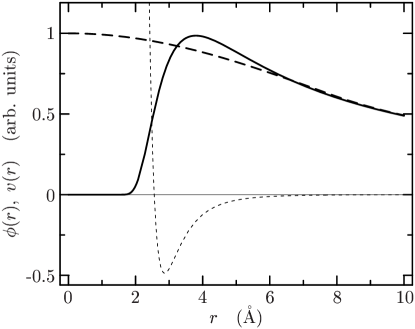
Figure 1: Exact relative wave function $\phi_{\mathrm{ex}}(r)$ for the $E=0$ scattering problem (solid line) in comparison with the hybrid ansatz $\phi_{0}(r)$ for $\xi=7.83\,\text{\AA}$ (dashed line). In addition the radial dependence of the Lennard-Jones potential $v(r)$ is shown (thin dotted line).

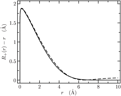
Figure 2: Optimal Correlation Function $R_{+}(r)-r$ resulting from the integral equation (45) (solid line) and the fitted parameterization (thin solid line). For comparison the parameterization with parameters resulting from energy minimization (thin dotted line) is depicted.

In Figure 1 the hybrid ansatz with matching radius $\chi=7.83\,\text{\AA}$ is shown in comparison with the exact $E=0$ solution. Both wave functions agree nicely at large distances. At small distances the exact solution shows the pronounced depletion within the core and an enhancement in the attractive region of the potential. These short-range correlations are not contained in the uncorrelated wave function (dashed curve). Instead the unitary correlation operator $\bm{C}$, which maps the uncorrelated wave function onto the exact eigenfunction (solid curve), takes over the task. As discussed in section II.3 this has the great advantage to allow the definition of correlated interactions that act between simple uncorrelated many-body states like product states.

The solution of the integral equation (45) for the correlation function $R_{+}(r)$ using these two wave functions is shown by the dashed line in Figure 2. The quantity $R_{+}(r)-r$ corresponds to the net distance by which two particles with an initial separation $r$ are shifted away from each other. The shape of the curve shows that particles with distances smaller than the core radius ($r_{\text{core}}\approx 2.5$Å) are shifted out of the core. If the initial distance is already larger than the core radius, then the shift decreases rapidly and finally vanishes at $r\approx 6.6$Å. The small shift for larger radii ($r>6.6$Å) originates from the minimal deviations of exact wave function and hybrid ansatz in this range. However these are long range correlations, which should not be described by the unitary correlation operator. Therefore we will set the function $R_{+}(r)-r$ to zero for $r\geq 6.6$Å in order to define the short-range correlation function.

This intrinsic separation between long- and short-range correlations works only if the potential has a sufficiently strong attractive region in addition to the repulsive core. For this class of interactions the exact two-body wave function is depleted inside the core and enhanced in the attractive region. Since the unitary correlation operator conserves the norm of the wave function it can generate this kind of structure very easily: The amplitude shifted out of the core is placed in the attractive region.

For purely repulsive potentials the situation is different. The exact wave function of a scattering state is depleted inside the core and the excess probability is spread over a large volume. Therefore the unitary mapping leads to a correlator of large range. In order to stay within the two-body approximation one has to restrict the range of the correlations and compensate by improving the uncorrelated trial states.

III.2 Energy Minimization

An alternative method to determine the correlation function $R_{+}(r)$ emerges from the variational principle. If we think of the energy expectation value to be calculated with correlated states and the uncorrelated Hamiltonian then the correlation function introduces additional degrees of freedom into the trial state. By choosing a suitable parameterization for $R_{+}(r)$ with few variational parameters we can minimize the correlated energy expectation value and obtain an optimal correlation function.

According to the structure of the correlation function determined by the mapping procedure described in the previous section we use the following parameterization

$$R_{+}(r)=r+\alpha\;(r/\beta)^{\eta}\;\exp[-\exp(r/\beta)]$$ (48)

with three free parameters. The parameter $\beta$ determines the range of the correlation function, $\alpha$ is related the maximum shift distance and thus the radius of the core, and $\eta$ influences the slope of $R_{+}(r)$ at small radii, i.e., the “hardness” of the core. We used this parameterization successfully for the description of the structure of atomic nuclei and nuclear matter UCOM98 ; Roth00 .

In order to describe a homogeneous ⁴He liquid we choose a constant wave function as two-body trial state $\big{<}{\vec{r}}\big{|}{\phi_{0}}\big{>}=1$. In that case only the local potentials $\tilde{v}(\bm{r})$ and $\tilde{u}(\bm{r})$ contribute to the expectation value of the correlated Hamiltonian

$$\begin{split}E=\big{<}{\phi_{0}}\big{|}\,{\tilde{\bm{H}}}\,\big{|}{\phi_{0}}\big{>}&=\big{<}{\phi_{0}}\big{|}\,{\tilde{v}(\bm{r})+\tilde{u}(\bm{r})}\,\big{|}{\phi_{0}}\big{>}\\ &=\int\!\!\mathrm{d}^{3}r\;[\tilde{v}(r)+\tilde{u}(r)].\end{split}$$ (49)

The expectation values of all momentum-dependent contributions $t_{\mathrm{rel}},\tilde{t}_{\Omega},\tilde{t}_{r}$ in (18) vanish. By inserting the parameterization of the correlation function into (16) and (21) we can express the integrand as function of the three variational parameters $\alpha,\beta$ and $\eta$. The integration as well as the minimization can easily be done numerically. We obtain a unique set of parameters for the optimal correlation function

$$\alpha=6.267\,\text{\AA},\quad\beta=3.520\,\text{\AA},\quad\eta=0.052.$$ (50)

The solid line in Figure 2 shows the resulting correlation function. It is in very good agreement with the correlation function determined by the mapping procedure (dashed line). This demonstrates that the parameterization used in the variation is well suited for the correlation function.

For numerical simplicity we will use the parameterized correlation function (48) with parameters according to (50) for the following investigations.

III.3 Correlated and Effective Interaction

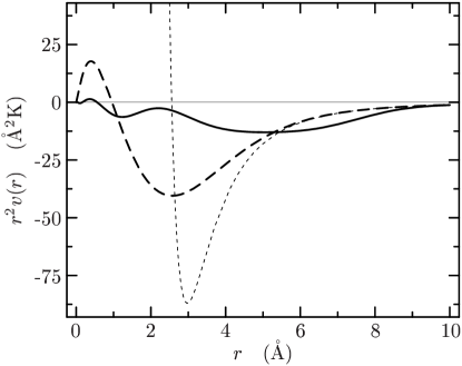
Figure 3: Local components of the correlated Hamiltonian: uncorrelated Lennard-Jones potential $r^{2}v(r)$ (thin dotted line), correlated potential $r^{2}\tilde{v}(r)$ (dashed line) and sum of correlated potential and local part of the correlated kinetic energy $r^{2}(\tilde{v}(r)+\tilde{u}(r))$ (solid line).

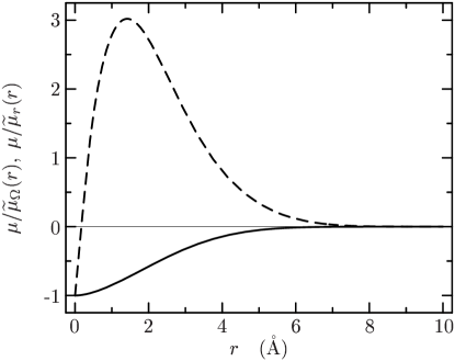
Figure 4: Radial dependencies of the effective mass corrections: angular effective mass correction $\mu/\tilde{\mu}_{\Omega}(r)$ (solid line) and radial effective mass correction $\mu/\tilde{\mu}_{r}(r)$ (dashed line).

With the explicit form of the correlation function we can study the structure of the correlated Hamiltonian in detail. As shown in section II.3 the unitary transformation generates a momentum-dependent effective interaction.

The local part of this interaction consists of the correlated interaction potential $\tilde{v}(r)$ (16) and a local contribution $\tilde{u}(r)$ (21) from the correlated kinetic energy operator. Figure 3 compares the radial dependencies of the uncorrelated Lennard-Jones potential, the correlated Lennard-Jones potential and the sum of all local contributions. The unitary transformation of the potential shifts the repulsive core to smaller radii. This leads to a substantial reduction of the strength of the core, only a moderate repulsion at very short ranges remains. If we add the local part of the correlated kinetic energy the repulsive part vanishes completely; the local component of the correlated Hamiltonian is purely attractive.

Actually, it can be shown analytically that mapping of an uncorrelated wave function, which is constant within the range of the repulsive core, onto the exact $E=0$ solution results in a local part $\tilde{v}(r)+\tilde{u}(r)$ of the correlated Hamiltonian that vanishes identically inside the core UCOM98 . The small contributions of the correlated local potentials within the core range that show up in Figure 3 result from the use of the restricted parameterization (48) for the correlation function and the slight variation of the trial state.

The momentum-dependent parts of the correlated Hamiltonian, which are formulated in terms of distance-dependent effective mass corrections (20), are shown in Figure 4. The radial effective mass correction (dashed line) generates a repulsion if the uncorrelated relative wave function has non-vanishing radial derivatives. The angular effective mass correction (solid line) generates an attraction if the uncorrelated wave function has non-vanishing relative angular momentum. In general the contribution of these components is small compared to the total energy expectation value as the uncorrelated states have small gradients.

Formally we can combine all the two-body terms of the correlated Hamiltonian to a momentum-dependent effective interaction

$$\tilde{\bm{w}}^{[2]}=\tilde{v}(\bm{r})+\tilde{u}(\bm{r})+\tilde{\bm{t}}_{\Omega}+\tilde{\bm{t}}_{r}$$ (51)

with a purely attractive local part given by (16) and (21) and a momentum dependence given by (19). With this effective interaction the correlated Hamiltonian in two-body approximation has the standard form

$$\tilde{\bm{H}}^{C2}=\bm{T}+\sum_{i<j}^{N}\tilde{\bm{w}}^{[2]}_{ij}.$$ (52)

The next orders of the cluster expansion contribute additional three-body, four-body, and higher order effective interactions.

The tamed effective two-body interaction $\tilde{\bm{w}}^{[2]}$ has a different operator structure and completely different radial dependencies than the uncorrelated potential $v(\bm{r})$. However, both interactions are phase-shift equivalent, i.e., in a two-body scattering process both interactions generate identical phase-shifts for any collision energy, by construction. This generic property of the effective interaction results from the finite range of the unitary transformation, which does not influence the asymptotic behavior of the scattering solutions. It is completely independent of the shape of the correlation function at short ranges. In that way the unitary correlator provides a recipe to generate an infinite manifold of phase-shift equivalent interactions. This aspect is of special interest in cases where the interaction is determined only on the basis of two-body scattering data — like the nucleon-nucleon interaction.

IV Homogeneous ⁴He-Liquid

As a first application of the UCOM formalism we want to investigate the equation of state, i.e., the energy per particle as function of the density, for a homogeneous ⁴He liquid at temperature $T=0$K.

In this case all effects that the interaction has on the many-body state are described by the unitary correlation operator. The uncorrelated many-body state $\,\big{|}{\Psi_{0}}\big{>}$ is a direct product of identical constant one-body states $\,\big{|}{\psi_{0}}\big{>}$

$$\,\big{|}{\Psi_{0}}\big{>}=\,\big{|}{\psi_{0}}\big{>}\otimes\cdots\otimes\,\big{|}{\psi_{0}}\big{>}.$$ (53)

For the calculation of expectation values we assume a finite volume $V$ containing $N$ particles. Accordingly the constant one-body states read

$$\big{<}{\vec{x}}\big{|}{\psi_{0}}\big{>}=V^{-1/2}.$$ (54)

The limit $N,V\to\infty$ at constant density $\rho=N/V$ is performed in the final step of the calculation.

IV.1 Equation of State in Two- and Three-Body Approximation

First we calculate the energy per particle with the correlated Hamiltonian in two-body approximation

$$\tilde{\bm{H}}^{C2}=\bm{T}+\tilde{\bm{V}}^{[2]}+\tilde{\bm{U}}^{[2]}+\tilde{\bm{T}}_{\Omega}^{[2]}+\tilde{\bm{T}}_{r}^{[2]}.$$ (55)

The energy per particle in two-body approximation is defined by the expectation value of this Hamiltonian calculated with the uncorrelated many-body state (53)

$$\tilde{\varepsilon}^{C2}(\rho)=\frac{1}{N}\big{<}{\Psi_{0}}\big{|}\,{\tilde{\bm{H}}^{C2}}\,\big{|}{\Psi_{0}}\big{>}.$$ (56)

Since the uncorrelated state is a product of constant one-body states only the local components $\tilde{\bm{V}}$ and $\tilde{\bm{U}}$ contribute; the expectation values of all momentum-dependent terms vanish. A simple calculation for the expectation value of the local components leads to the following expression for the energy per particle in two-body approximation

$$\tilde{\varepsilon}^{C2}(\rho)=(C_{v}^{[2]}+C_{u}^{[2]})\;\rho$$ (57)

with constant coefficients given by

$$C_{v}^{[2]}=\frac{1}{2}\int\!\!\mathrm{d}^{3}r\;\tilde{v}(r),\qquad C_{u}^{[2]}=\frac{1}{2}\int\!\!\mathrm{d}^{3}r\;\tilde{u}(r).$$ (58)

The integrals over the correlated potential $\tilde{v}(r)$ given by (16) and the local part of the correlated kinetic energy $\tilde{u}(r)$ according to (21) are evaluated numerically

$$C_{v}^{[2]}=-856.5\,\text{K\AA}^{3},\qquad C_{u}^{[2]}=401.5\,\text{K\AA}^{3}.$$ (59)

Obviously, for homogeneous Bose fluids at zero temperature the two-body approximation is not able to describe saturation, i.e., a minimum of the energy at some finite density. The energy in two-body approximation (57) is always proportional to density and due to the negative sum of the coefficients (59) drops with increasing density.

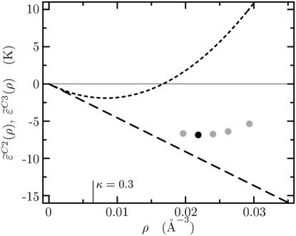
Figure 5: Energy per particle for a homogeneous ⁴He liquid as function of density calculated in two-body approximation $\tilde{\varepsilon}^{C2}(\rho)$ (dashed line) and in three-body approximation $\tilde{\varepsilon}^{C3}(\rho)$ (dotted line). The vertical line marks the density at which the smallness parameter $\kappa$ reaches the value $0.3$. The circles show the results of an exact GFMC calculation KaLe81 ; statistical errors are smaller than the size of the symbols.

The dashed line in Figure 5 shows this behavior in comparison with results of a Green’s Function Monte Carlo (GFMC) calculation KaLe81 , which are exact up to the statistical errors of the Monte Carlo sampling. Despite the fact that the two-body approximation fails to generate a minimum, the predicted orders of magnitude for the energy are correct. This is remarkable, considering that the uncorrelated Lennard-Jones potential would give an infinite positive energy expectation value for all densities. The special unitary transformation that we apply tames the strong core of the potential and leads to a bound many-body system.

We note that the two-body approximation does generate saturation in other systems like homogeneous Fermi liquids. In these cases the mass corrections contribute, because of the Fermi motion, and generate a positive contribution to the energy that grows with a higher power in density than the attractive local terms.

A straightforward step to go beyond the two-body approximation is the inclusion of the three-body terms of the cluster expansion. In addition to the terms in (55) the correlated Hamiltonian in three-body approximation contains three-body contributions from the correlated potential and the correlated kinetic energy

$$\tilde{\bm{H}}^{C3}=\tilde{\bm{H}}^{C2}+\tilde{\bm{V}}^{[3]}+\tilde{\bm{U}}^{[3]}+\tilde{\bm{T}}^{[3]}.$$ (60)

Again only the local three-body terms $\tilde{\bm{V}}^{[3]}$ and $\tilde{\bm{U}}^{[3]}$ contribute to the energy expectation value with the uncorrelated states (53). The resulting energy per particle in three-body approximation reads

$$\tilde{\varepsilon}^{C3}(\rho)=(C_{v}^{[2]}+C_{u}^{[2]})\;\rho+(C_{v}^{[3]}+C_{u}^{[3]})\;\rho^{2}.$$ (61)

The coefficients are defined by the six-dimensional integrals

$$C_{v}^{[3]}=\frac{1}{6}\int\!\!\mathrm{d}^{3}x_{1}\mathrm{d}^{3}x_{2}\;\tilde{v}^{[3]}(\vec{x}_{1},\vec{x}_{2},\vec{x}_{3}=0)$$ (62)

and the corresponding expression for $C_{u}^{[3]}$. The integration is done with a standard Monte Carlo algorithm (“VEGAS” from PrTe92 ) and yields

$$\begin{split}C_{v}^{[3]}&=(-2512\pm 50)\,\text{K\AA}^{6},\\ C_{u}^{[3]}&=(29739\pm 1100)\,\text{K\AA}^{6}.\end{split}$$ (63)

The local three-body terms of the correlated Hamiltonian generate a positive contribution to the energy per particle which is proportional to $\rho^{2}$. The dominant term is the local three-body contribution of the correlated kinetic energy. Together with the negative density-proportional contribution of the local two-body potentials the energy in three-body approximation (61) provides a minimum at finite density.

The density dependence of the energy per particle in three-body approximation $\tilde{\varepsilon}^{C3}(\rho)$ is shown by the dotted curve in Figure 5. Obviously the three-body contribution is not a small correction to the two-body approximation for densities larger than $0.005\,\text{\AA}^{-3}$, which is only one fourth of the saturation density. This demonstrates that many-body correlations have a strong influence in these systems and that the two-body approximation alone is not sufficient to describe ground state properties. A similar conclusion can be drawn from the smallness parameter $\kappa=\rho\,V_{C}$. It reaches the phenomenological limit $\kappa=0.3$ for the validity of the two-body approximation at about $1/3$ of the expected saturation density .

However, the naive inclusion of the three-body terms of the cluster expansion of the correlated Hamiltonian does not improve the result beyond a density of about $0.005\,\text{\AA}^{-3}$. Although we obtain saturation in three-body approximation, both, energy and density at the minimum of $\tilde{\varepsilon}^{C3}(\rho)$ are substantially smaller than the results of the GFMC calculation. This discrepancy has several reasons: Firstly, the optimal correlation function was determined in the two-body system, i.e., in two-body approximation. For a consistent treatment on the level of the three-body approximation the optimal correlation function should be determined by minimizing the energy in three-body approximation. Secondly, we expect that genuine three-body correlations play a very strong role UsFa82 ; Pand78 . They are described by an irreducible three-body part $\sum_{i<j<k}\bm{g}_{ijk}$ in the generator (3) that was not included in the present treatment. Finally, in view of the large three-body contributions there is no good reason to neglect terms beyond three-body order.

Each of the points mentioned can in principle be explicitly included in the calculation. However, none of these corrections are expected to yield reasonably converged results in the particular case of the ⁴He liquid. The density range where the description should be applied is far above the range where the two-body approximation is applicable, i.e., where the smallness parameter $\kappa$ is below the typical value of $0.3$. The successive inclusion of higher orders of the cluster expansion will extend this range but one would have to include very high orders — which are beyond the numerical possibilities — to reach the expected saturation density. The only reasonable way to extend the treatment is a partial summation over all cluster orders. This is done in the framework of Jastrow correlations with the so called Hypernetted Chain (HNC) summation schemes PaSc77 ; Pand78 ; Clar79 ; UsFa82 . However, this type of partial summation is not feasible for the unitary correlation operator because of its more complicated operator structure.

IV.2 Equation of State with Density-Dependent Correlation Functions

We aim at an effective description of the higher orders of the cluster expansion that still allows a compact analytic formulation of correlated observables and does not require extensive numerical efforts. One general way to simulate the effect of higher cluster orders is to introduce density-dependent correlation functions on the level of the two-body approximation.

At low densities the correlator shifts a pair of particles in an optimal way from the repulsive into the attractive region. When the density grows other particles will be nearby and obstruct the correlation that was optimal for a free particle pair. To simulate this effect the range of the correlation function $R_{+}(r)$ should be more and more reduced for increasing density. This will reduce the binding as the particles will not be able any more to fully exploit the attractive region of the potential.

In practice this is accomplished by scaling the parameters $\alpha$ and $\beta$, which have the dimension of a length, in the parameterization (48) of the correlation function $R_{+}(r)$ with some factor $\xi(\rho)\lesssim 1$ that depends on density. At very low densities we assume that the higher-order contributions are negligible such that $\xi(\rho\to 0)=1$. With growing density the effect of the higher cluster orders grows such that the scaling factor $\xi(\rho)$ has to drop. The most simple ansatz for the density dependence of $\xi(\rho)$ is

$$\xi(\rho)=1-\gamma\rho,$$ (64)

with one free parameter $\gamma$. The density-dependent correlation function reads

$$R_{+}(r,\rho)=r+\alpha\xi(\rho)\Big{[}\frac{r}{\beta\xi(\rho)}\Big{]}^{\!\eta}\exp\!\!\Big{[}\!\!-\exp\!\Big{(}\frac{r}{\beta\xi(\rho)}\Big{)}\!\Big{]}.$$ (65)

Using this correlation function all components of the correlated Hamiltonian — like correlated potential, local part of the correlated kinetic energy, and effective mass corrections — become explicitly density-dependent. The energy per particle is given by

$$\tilde{\varepsilon}^{C2}_{\rho}(\rho)=\frac{\rho}{2}\int\!\!\mathrm{d}^{3}r\;[\tilde{v}_{\rho}(r,\rho)+\tilde{u}_{\rho}(r,\rho)],$$ (66)

where the subscript $\rho$ indicates that the density-dependent correlation function is used.

Due to the explicit density-dependence of the correlated local potentials the equation of state is not proportional to $\rho$ any more. From a Taylor expansion of (66) around $\rho=0$ we obtain terms to all powers of the density. Thus all orders of the cluster expansion are represented by the density-dependent correlator in an effective way.

The phenomenological parameter $\gamma$ in the scaling factor (64) is in general adjusted such that (66) agrees with one experimental data point, or for some density with the result of a realistic calculation. We will use the result of the GFMC calculation KaLe81 for the density $\rho^{\text{GFMC}}_{\mathrm{sat}}$ and energy $\varepsilon^{\text{GFMC}}_{\mathrm{sat}}$ at the saturation point and require

$$\tilde{\varepsilon}^{C2}_{\rho}(\rho^{\text{GFMC}}_{\mathrm{sat}})\overset{!}{=}\varepsilon^{\text{GFMC}}_{\mathrm{sat}}.$$ (67)

This ensures that the equation of state (66) calculated with the density-dependent correlator runs through that point. However, this does not imply that the minimum of (66) coincides with the GFMC minimum. Using the values KaLe81 $\rho^{\text{GFMC}}_{\mathrm{sat}}=0.0219\,\text{\AA}^{-3}$ and $\varepsilon^{\text{GFMC}}_{\mathrm{sat}}=-6.848\,\text{K}$ we obtain

$$\gamma=3.696\,\text{\AA}^{3}.$$ (68)

We have chosen to fix the density dependence, i.e., $\gamma$, with a calculation instead of an experimental value, because that calculation uses the same potential (1) and it is known that this simple Lennard-Jones potential does not reproduce exactly the experimental two-body data.

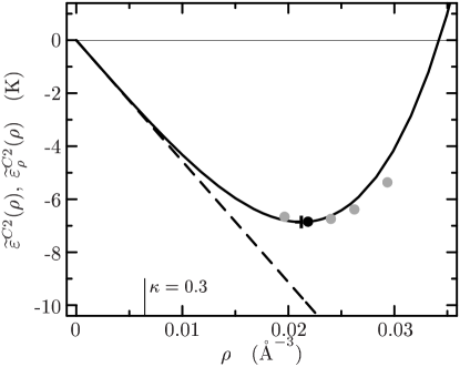
Figure 6: Energy per particle for a homogeneous ⁴He liquid calculated in two-body approximation with a two-body optimized correlation function $\tilde{\varepsilon}^{C2}(\rho)$ (dashed line) and with density-dependent correlation function $\tilde{\varepsilon}^{C2}_{\rho}(\rho)$ (solid line). The vertical line marks the density at which the smallness parameter $\kappa$ reaches the value $0.3$. The gray circles show the results of an exact GFMC calculation KaLe81 , the minimum is indicated by the black circle.

Figure 6 shows the energy per particle $\tilde{\varepsilon}^{C2}_{\rho}(\rho)$ calculated with the density-dependent correlation function. The phenomenological description of the higher order contributions by a density-dependent correlation function indeed generates a minimum of the energy with

$$\rho_{\mathrm{sat}}=0.0212\,\text{\AA}^{-3},\qquad\tilde{\varepsilon}^{C2}_{\rho,\mathrm{sat}}=-6.860\,\text{K}.$$ (69)

The position of the minimum (indicated by the cross) as well as the shape of the equation of state around the minimum agree very nicely the the GFMC result. As noted above this is not an immediate consequence of the adjustment of $\gamma$. The agreement shows that the phenomenological density-dependence is well suited to describe the major aspects of many-body correlations on a numerically very simple level. Actually, all calculations have been performed within a simple Mathematica notebook.

Once the density-dependence is fixed the correlation function can be used to evaluate any correlated observable of interest. The analytic expressions for many correlated observables in two-body approximation are rather simple, but the evaluation of higher cluster orders becomes complicated if not intractable. Thus the inclusion of the phenomenological treatment of higher order effects by means of the density-dependent correlator is a very useful tool. Interesting quantities are, e.g., the radial two-body distribution function $g(r)$, the static structure factor $S(q)$ or the one-body momentum distribution $n(k)$. The corresponding observables for fermionic liquids were discussed elsewhere Roth00 .

In the following section we will use the density-dependent correlation function to investigate the structure of small droplets of ⁴He. This will demonstrate the universality of the concept.

V Small ⁴He-Droplets

In a next step we want to use the Unitary Correlation Operator Method to investigate the ground state properties of small ⁴He droplets.

The many-body problem is treated in a simple variational framework. The many-body trial state $\,\big{|}{\Psi,N}\big{>}$ is — like for the homogeneous liquid — assumed to be a direct product of identical one-body states. The one-body states are described by a Gaussian wave function

$$\big{<}{\vec{x}}\big{|}{\psi}\big{>}=(\pi a)^{-3/4}\exp[-\vec{x}^{2}/(2a)]$$ (70)

with a common width parameter $a$ as the only variational degree of freedom. The Gaussian trial state is applicable for small droplets with $N\lesssim 70$; larger droplets show a saturation of the central density, which cannot be modeled with this ansatz PaPi86 ; KrCh95 . An advantage of the Gaussian ansatz is that the two-body wave function

$$\big{<}{\vec{x}_{1},\vec{x}_{2}}\big{|}{\psi,\psi}\big{>}=\big{<}{\vec{X}}\big{|}{\Phi}\big{>}\big{<}{\vec{r}}\big{|}{\phi}\big{>}$$ (71)

can be separated analytically into a center of mass component $\big{<}{\vec{X}}\big{|}{\Phi}\big{>}$ and a relative wave function $\big{<}{\vec{r}}\big{|}{\phi}\big{>}$

$$\begin{split}\big{<}{\vec{X}}\big{|}{\Phi}\big{>}&=(\pi a/2)^{-3/4}\exp[-\vec{X}^{2}\!/a],\\ \big{<}{\vec{r}}\big{|}{\phi}\big{>}&=(2\pi a)^{-3/4}\exp[-\vec{r}^{\,2}\!/(4a)].\end{split}$$ (72)

This simple trial state is able to describe mean-field like effects of the interaction, i.e., the spatial localization of the atoms. However, any correlation effect beyond the mean-field level has to be described by the unitary correlation operator.

V.1 Binding Energy and rms-Radius in Two-Body Approximation

First we use the two-body approximation with the correlation function (48) obtained from the two-body scattering solution to investigate the ground state properties of small droplets. The correlated intrinsic Hamiltonian $\tilde{\bm{H}}^{C2}_{\mathrm{int}}=\tilde{\bm{H}}^{C2}-\bm{T}_{\mathrm{cm}}$ in two-body approximation has the structure

$$\tilde{\bm{H}}^{C2}_{\mathrm{int}}=\bm{T}_{\mathrm{int}}+\tilde{\bm{V}}^{[2]}+\tilde{\bm{U}}^{[2]}+\tilde{\bm{T}}_{\Omega}^{[2]}+\tilde{\bm{T}}_{r}^{[2]},$$ (73)

where capital letters indicate summation over all particles, like $\tilde{\bm{V}}^{[2]}=\sum_{i<j}^{N}\tilde{\bm{v}}^{[2]}_{ij}$. The uncorrelated intrinsic kinetic energy $\bm{T}_{\mathrm{int}}$, i.e., the total kinetic energy $\bm{T}$ reduced by the center of mass contribution $\bm{T}_{\mathrm{cm}}$, can be expressed by the relative two-body kinetic energy $\bm{t}_{\mathrm{rel}}$

$$\bm{T}_{\mathrm{int}}=\bm{T}-\bm{T}_{\mathrm{cm}}=\frac{2}{N}\sum_{i<j}^{N}\bm{t}_{\mathrm{rel},ij},$$ (74)

where

$$\bm{T}=\frac{1}{2m}\sum_{i}^{N}\vec{\bm{p}}_{i}^{2}\;,\qquad\bm{T}_{\mathrm{cm}}=\frac{1}{2mN}\bigg{[}\sum_{i}^{N}\vec{\bm{p}}_{i}\bigg{]}^{2}.$$ (75)

Due to the simple structure of the many-body trial state the expectation value of the correlated Hamiltonian (73) in the $N$-body system can be expressed by that of the two-body system

$$\begin{split}\tilde{E}^{C2}&=\big{<}{\Psi,N}\big{|}\,{\tilde{\bm{H}}^{C2}_{\mathrm{int}}}\,\big{|}{\Psi,N}\big{>}\\ &=\frac{N(N-1)}{2}\big{<}{\Psi,2}\big{|}\,{\tilde{\bm{H}}^{C2}_{\mathrm{int}}}\,\big{|}{\Psi,2}\big{>}.\end{split}$$ (76)

Moreover we can use that the intrinsic Hamiltonian (73) acts on the relative part $\big{<}{\vec{r}}\big{|}{\phi}\big{>}$ of the two-body wave function only. This leads to a simple form of the correlated energy expectation value of the $N$-body system

$$\begin{split}\tilde{E}^{C2}&=(N-1)\;\big{<}{\phi}\big{|}\,{\bm{t}_{\mathrm{rel}}}\,\big{|}{\phi}\big{>}\\ &+\frac{N(N-1)}{2}\big{<}{\phi}\big{|}\,{\tilde{v}(\bm{r})+\tilde{u}(\bm{r})+\tilde{\bm{t}}_{r}}\,\big{|}{\phi}\big{>}.\end{split}$$ (77)

We used that the expectation value of the angular effective mass correction $\tilde{t}_{\Omega}$ vanishes due to the spherical symmetry of the relative wave function (relative s-wave state). The two-body expectation value of the relative kinetic energy is given by

$$\big{<}{\phi}\big{|}\,{\bm{t}_{\mathrm{rel}}}\,\big{|}{\phi}\big{>}=\frac{1}{2\mu}\int\!\!\mathrm{d}^{3}r\;\Big{|}\frac{\partial}{\partial r}\big{<}{r}\big{|}{\phi}\big{>}\Big{|}^{2}=\frac{1}{2\mu}\frac{3}{4a}.$$ (78)

For the correlated two-body potential and the local part of the correlated kinetic energy we obtain

$$\big{<}{\phi}\big{|}\,{\tilde{v}(\bm{r})+\tilde{u}(\bm{r})}\,\big{|}{\phi}\big{>}=\int\!\!\mathrm{d}^{3}r\;[\tilde{v}(r)+\tilde{u}(r)]\;\big{|}\big{<}{r}\big{|}{\phi}\big{>}\big{|}^{2}.$$ (79)

Finally, the expectation value of the radial effective mass correction reads

$$\big{<}{\phi}\big{|}\,{\tilde{\bm{t}}_{r}}\,\big{|}{\phi}\big{>}=\frac{1}{2\mu}\int\!\!\mathrm{d}^{3}r\;\frac{\mu}{\tilde{\mu}_{r}(r)}\Big{|}\frac{\partial}{\partial r}\big{<}{r}\big{|}{\phi}\big{>}\Big{|}^{2}.$$ (80)

For a fixed correlation function $R_{+}(r)$ the radial dependencies of the correlated potential $\tilde{v}(r)$, the local part of the correlated kinetic energy $\tilde{u}(r)$, and the radial effective mass correction $\mu/\tilde{\mu}_{r}(r)$ are known analytically (see section II.3). The minimization of the energy $\tilde{E}^{C2}$ as function of the width parameter $a$ as well as the calculation of the integrals in equations (79) and (80) is done numerically.

Another interesting observable is the mean-square radius of the droplet, defined by the expectation value of the operator

$$\bm{R}_{\text{ms}}=\frac{1}{N}\sum_{i}^{N}(\vec{\bm{x}}_{i}-\vec{\bm{X}}_{\mathrm{cm}})^{2}=\frac{1}{N^{2}}\sum_{i<j}^{N}\bm{r}_{ij}^{2},$$ (81)

where $\vec{\bm{X}}_{\mathrm{cm}}=\frac{1}{N}\sum_{i}^{N}\vec{\bm{x}}_{i}$ is the center of mass coordinate of the many-body system. The formulation in terms of the two-body operator $\bm{r}^{2}$ reveals a similar structure like for the intrinsic kinetic energy (74). The many-body product state under consideration allows a direct calculation of the uncorrelated expectation value using the relative two-body wave function (72)

$$\begin{split}r_{\text{rms}}&=\big{[}\big{<}{\Psi,N}\big{|}\,{\bm{R}_{\text{ms}}}\,\big{|}{\Psi,N}\big{>}\big{]}^{1/2}\\ &=\bigg{[}\frac{N-1}{2N}\big{<}{\phi}\big{|}\,{\bm{r}^{2}}\,\big{|}{\phi}\big{>}\bigg{]}^{1/2}=\bigg{[}\frac{N-1}{2N}\,3a\bigg{]}^{1/2}.\end{split}$$ (82)

The correlated ms-radius $\tilde{\bm{R}}_{\text{ms}}^{C2}$ in two-body approximation has a similar structure like the kinetic energy

$$\tilde{\bm{R}}_{\text{ms}}^{C2}=\bm{R}_{\text{ms}}+\tilde{\bm{R}}_{\text{ms}}^{[2]}.$$ (83)

In addition to the uncorrelated mean-square radius $\bm{R}_{\text{ms}}$ the unitary transformation generates a two-body contribution

$$\tilde{\bm{R}}_{\text{ms}}^{[2]}=\frac{1}{2N}\sum_{i<j}^{N}\big{[}R_{+}^{2}(\bm{r}_{ij})-\bm{r}_{ij}^{2}\big{]}.$$ (84)

The expectation value of the correlated ms-radius (83) can again be expressed by the relative two-body wave function alone

$$\tilde{r}_{\text{rms}}^{C2}=\bigg{[}\frac{N-1}{2N}\big{<}{\phi}\big{|}\,{\bm{r}^{2}+\frac{N}{2}\big{(}R_{+}^{2}(\bm{r})-\bm{r}^{2}\big{)}}\,\big{|}{\phi}\big{>}\bigg{]}^{1/2}.$$ (85)

In order to study the quality of the two-body approximation we first look at very small droplets with $N\leq 10$. For these droplet sizes an early variational Monte Carlo (VMC) calculation on the basis of the Lennard-Jones potential exists ScSc65 . The authors use a Jastrow-type parameterization of two-body correlations with a long-range form adjusted to the behavior of the exact two-body solution. The calculation of the many-body expectation value with these trial states involves a Monte Carlo integration routine. The resulting energy expectation values show a statistical error of approximately 10%.

Our results of the minimization of $\tilde{E}^{C2}$ (77) with respect to $a$ using the system independent correlation function given in equations (48) and (50) for $N\leq 10$ are summarized in Figure 7. The upper panel shows the correlated energy per particle, the middle panel the correlated rms-radius of the droplet and the lower panel the smallness parameter $\kappa_{\mathrm{eq}}$ versus the number of particles $N$.

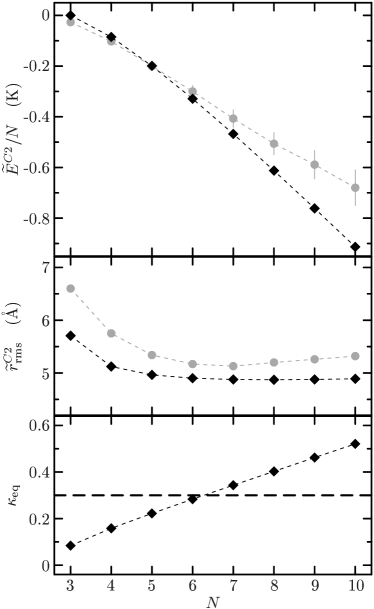
Figure 7: Energy per particle (upper panel), rms-Radius (middle panel), and smallness parameter $\kappa_{\mathrm{eq}}$ (lower panel) for small ⁴He droplets in two-body approximation with two-body optimized correlation function. The gray circles show results of a variational Monte Carlo calculation ScSc65 , statistical errors for the energy are indicated by the gray bars. The lines should guide the eye.

As for the homogeneous liquid the expectation values of the uncorrelated Lennard-Jones potential would diverge. But the unitary transformation of the Hamiltonian using the correlation function determined in the two-body system removes the strong short-range repulsion of the potential completely. With this tamed correlated potential and a simple product ansatz for the many-body wave function the energies of very loosely bound droplets actually agree very nicely for $N\leq 6$ with the VMC result. For $N>6$ the energy expectation value is below the VMC value and the difference grows with increasing particle number or density. Since expectation values are evaluated in two-body approximation, i.e., the full cluster expansion is truncated above two-body order, a basic property of the Ritz variational principle is lost: The variational minimum of the energy is not necessarily bounded from below by the exact energy eigenvalue. The observed overbinding indicates that the higher orders of the cluster expansion have to give a sizeable positive contribution to raise the expectation value above the exact eigenvalue.

In direct connection with the overbinding in two-body approximation the correlated rms-radii of energy minimized states are systematically smaller than the VMC result. Accordingly the densities are too high. In contrast to the homogeneous liquid the two-body approximation does not produce a pathological collapse towards high densities for small droplets. This is due to the positive contributions of the kinetic energy and the effective mass correction that are absent in the homogeneous case.

As a measure for the validity of the two-body approximation we used the smallness parameter $\kappa=\rho V_{C}$ with correlation volume $V_{C}$ defined by (28). In order to specify the smallness parameter for inhomogeneous systems we have to define a measure for the average density. One possible definition is the value of the density for a step-like density profile with same (uncorrelated) rms-radius as the original distribution. For identical Gaussian single-particle wave functions with width parameter $a$ this equivalent density is given by

$$\rho_{\mathrm{eq}}=\frac{3N}{4\pi}\bigg{[}\frac{3}{5}\;\frac{1}{r_{\text{rms}}^{2}}\bigg{]}^{3/2}=\frac{3N}{4\pi}\bigg{[}\frac{2}{5}\;\frac{N}{N-1}\;\frac{1}{a}\bigg{]}^{3/2}.$$ (86)

The smallness parameter $\kappa_{\mathrm{eq}}=\rho_{\mathrm{eq}}V_{C}$ defined with this density is shown in the lower panel of Figure 7 as function of particle number. Like for the homogeneous liquid the energy in two-body approximation starts to deviate from the exact result if the smallness parameter $\kappa_{\mathrm{eq}}$ exceeds the value $0.3$ (indicated by the dashed line). This again confirms that the two-body approximation is valid as long as the smallness parameter fulfills the condition $\kappa\lesssim 0.3$.

V.2 Energy and rms-Radius with Density-Dependent Correlation Function

To account for the effect of many-body correlations in a simple but efficient way we employ the concept of density-dependent correlation functions introduced in section IV.2 for the homogeneous liquid.

To apply the density-dependent correlator in an inhomogeneous system we have to specify in which way the density-dependence should be evaluated. The most simple approach is to insert the equivalent density of the droplet, as defined in (86), into the density-dependent correlation function. That means we neglect that the effects from stronger many-body correlations in the center of the droplet do not exactly cancel the weaker ones at the surface.

A more elaborate ansatz to account for the inhomogeneity would be to implement the density-dependence in local density approximation, i.e., the correlation function which acts on the relative coordinate of a particle pair depends on the local density at their center of mass position. This is not done here.

Table 1: Energy expectation values and rms-radii for small ⁴He droplets with different particle number $N$ resulting from energy minimization in two-body approximation with two-body optimized and density-dependent correlation function. The width parameter $a$ is given in units of Ų, energies are given per particle in units of K, and the rms-radius in units of Å.

	Two-Body Approximation			Two-Body Approximation with Density-Dependent Correlator							Ref. ScSc65
$N$	$a$	$\tilde{E}^{C2}\!/N$	$\tilde{r}_{\text{rms}}^{C2}$	$a$	$T_{\text{int}}/N$	$\tilde{T}_{r,\rho}^{[2]}/N$	$\tilde{U}^{[2]}_{\rho}/N$	$\tilde{V}^{[2]}_{\rho}/N$	$\tilde{E}^{C2}_{\rho}\!/N$	$\tilde{r}_{\text{rms},\rho}^{C2}$	$E/N$	$r_{\text{rms}}$
3	32.33	0.000	5.71	34.39	0.176	0.005	0.238	-0.418	0.002	5.88	-0.027	6.60
4	22.83	-0.085	5.12	25.19	0.271	0.021	0.551	-0.919	-0.076	5.37	-0.103	5.75
5	19.81	-0.199	4.97	22.70	0.320	0.038	0.846	-1.379	-0.175	5.29	-0.200	5.34
6	18.26	-0.329	4.90	21.71	0.349	0.054	1.122	-1.807	-0.282	5.30	-0.300	5.17
7	17.31	-0.468	4.88	21.32	0.366	0.067	1.378	-2.202	-0.391	5.34	-0.407	5.13
8	16.67	-0.613	4.87	21.23	0.375	0.079	1.614	-2.567	-0.500	5.40	-0.506	5.20
9	16.20	-0.761	4.88	21.31	0.379	0.088	1.832	-2.905	-0.606	5.46	-0.589	5.26
10	15.84	-0.913	4.89	21.50	0.380	0.096	2.033	-3.218	-0.709	5.53	-0.680	5.32
20	14.42	-2.500	5.14	25.13	0.343	0.118	3.427	-5.442	-1.554	6.20
30	14.01	-4.125	5.44	29.15	0.301	0.109	4.221	-6.778	-2.146	6.75
40	13.81	-5.760	5.74	32.97	0.269	0.098	4.745	-7.698	-2.588	7.20
50	13.69	-7.399	6.02	36.59	0.243	0.085	5.119	-8.381	-2.933	7.60
60	13.61	-9.040	6.29	40.02	0.223	0.076	5.405	-8.918	-3.214	7.95
70	13.56	-10.683	6.55	43.29	0.207	0.068	5.631	-9.353	-3.447	8.26

The variational calculation of the ground state properties of small ⁴He droplets including a correlation function that depends on the equivalent density (86) is straightforward. The parameterization (65) of the correlation function $R_{+}(r,\rho_{\mathrm{eq}})$ is used with the parameters (50) determined in the two-body system. The parameter of the density-dependent scaling function (64) is taken from the investigations of the homogeneous liquid (68). The energy expectation value in two-body approximation with density-dependent correlations is of the same form as for the density-independent correlation functions discussed in the preceding section.

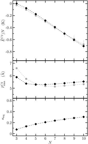
Figure 8: Energy per particle (upper panel), rms-Radius (middle panel), and smallness parameter $\kappa_{\mathrm{eq}}$ (lower panel) for small ⁴He droplets in two-body approximation with the density-dependent correlation function fixed in the homogeneous liquid. The gray circles show results of a variational Monte Carlo calculation ScSc65 . The lines should guide the eye.

The results of the energy minimization with respect to the width parameter $a$ are summarized in Figure 8. The energy expectation values are in full agreement with the VMC calculation ScSc65 for all particle numbers. The overbinding observed with a density-independent correlation function is completely compensated by the density-dependence. The correlated rms-radii of droplets with $N\geq 6$ are consistently larger by 0.2Å than the VMC result. Unfortunately the authors ScSc65 give no estimate for the statistical or systematic errors for their procedure to obtain the rms-radii. For the smallest droplets our result for the rms-radii are below the VMC results. This may be caused by the restriction to Gaussian trial states (72), which are not able to describe the long-range exponential tail present in these extremely weakly bound systems. At the same time the insufficient trial state causes a slight underbinding of the smallest droplets.

For completeness Figure 8 also shows the smallness parameter $\kappa_{\mathrm{eq}}=\rho_{\mathrm{eq}}V_{C}$. Since both, the correlation volume $V_{C}$ and the density of the droplets are reduced by the density-dependent correlator the product stays small. In any case $\kappa_{\mathrm{eq}}$ has lost its meaning as a measure for three-body correlations as the density-dependence of the correlator already includes many-body correlations.

Table 1 summarizes the results of the energy minimization with two-body optimized and density-dependent correlator for droplet sizes up to $N=70$. In addition to the correlated energy and the rms-radius the individual terms of the correlated Hamiltonian are shown. The attractive correlated potential and the repulsive local part of the correlated kinetic energy are the major contributions and show a large cancellation. The intrinsic kinetic energy and the effective mass correction give rather small contributions.

VI Summary and Conclusions

We presented a simple and elegant approach to describe strong short-range correlations in a many-body system that result from the strong repulsive core of the two-body interaction. These correlations induce high-momentum components into the relative wave function that cannot be treated within a low-momentum model space. The correlation operator $\bm{C}$ generates the short-range correlations by a unitary transformation in the relative coordinate of each pair of particles. It shifts the particles out of the repulsive core of the two-body interaction.

The correlation operator is then used to define correlated observables, most notably the correlated Hamiltonian. The unitary transformation yields a tamed effective two-body interaction, which consists of a purely attractive local part and a weak momentum dependence. In addition three-body and higher order terms are generated. For dilute systems, i.e., if the range of the correlations is small compared to the average distance between the particles, it is sufficient to include the terms up to two-body order. In high-density systems the higher order terms can be included explicitly or simulated by a density-dependent correlation function.

In order to study the applicability of the method in many-body systems, where short-range correlations play a dominant role, we investigated the ground state properties of homogeneous ⁴He liquids and small droplets. The correlation function is fixed by energy minimization in the two-body problem with a constant uncorrelated wave function. Alternatively the correlation function can be determined by mapping an uncorrelated wave function onto the exact energy $E=0$ two-body wave function.

We use this correlation function to calculate the energy of the homogeneous ⁴He liquid as function of density. The uncorrelated many-body state is a direct product of constant one-body states, thus the influence of the interaction on the state has to be described by the correlation operator alone. Already in two-body approximation the strong short-range repulsion of the Lennard-Jones potential is tamed completely and we obtain a bound system. However, the two-body approximation does not generate saturation, i.e., the energy per particle decreases proportional to density. To simulate the effect of many-body correlations we employ a density-dependent correlation function. The one parameter introduced by the density dependent scaling of the correlation function is fixed by adjusting the correlated energy for one value of the density to the result of a GFMC calculation. The resulting equation of state shows a minimum and is in very good agreement with the predictions of the GFMC calculation over the whole density range.

In a second step we use the density-independent as well as the density-dependent correlation function to perform an ab initio calculation of the ground state structure of small ⁴He droplets in a simple variational framework. It turns out that the two-body approximation with the density-independent correlation function gives a good description for small droplets with particle numbers $N\leq 6$. For larger droplets an overbinding compared to a quasi exact variational Monte Carlo calculation appears. Due to the higher density in these droplets many-body correlations become relevant. If we use the density-dependent correlation function with one parameter adjusted in the homogeneous liquid then the energies and rms-radii are in very good agreement with the exact calculation for all particle numbers under consideration.

We conclude that the Unitary Correlation Operator Method is a powerful and universal tool to handle short-range correlations in the many-body system. For sufficiently low densities one can use the two-body approximation to construct the correlated Hamiltonian as well as other correlated observables in closed form. The resulting effective two-body interaction can be used for an ab initio description of the many-body system based on a low-momentum model space. A gross measure for the validity of the two-body approximation is the smallness parameter $\kappa$ (27), which should be below a phenomenological limit of $0.3$.

For higher densities one can utilize density-dependent correlation functions to describe many-body correlations effectively within the two-body approximation. The additional parameter in the density-dependence can be fixed by one measured data point or by comparison with an exact calculation. Nevertheless, the resulting density-dependent correlator can then be used for a broad range of applications, e.g., ab initio calculations of correlated observables like energies, densities or momentum distributions of different systems without further adjustments. The great advantage of the Unitary Correlation Operator Method with density-dependent correlation functions is that besides its transparent physics it requires only minimal computational power compared to the huge computational resources needed for Monte-Carlo-type calculations. A set of Mathematica notebooks that illustrate the application of the Unitary Correlation Operator Method to ⁴He liquids can be found at the URL: http://theory.gsi.de/~rroth/math/.

References

- (1) R. A. Aziz, V. P. S. Nain, J. S. Carley, W. L. Taylor, and G. T. McConville, J. Chem. Phys. 70, 4330 (1979).
- (2) J. de Boer and A. Michels, Physica 6, 945 (1938).
- (3) C.-W. Woo, in The Physics of Liquid and Solid Helium, edited by K. H. Bennemann and J. B. Ketterson (Wiley Interscience, 1981), vol. I.
- (4) H. Feldmeier, T. Neff, R. Roth, and J. Schnack, Nucl. Phys. A632, 61 (1998).
- (5) M. H. Kalos, M. A. Lee, P. A. Whitlock, and G. V. Chester, Phys. Rev. B 24, 115 (1981).
- (6) E. W. Schmid, J. Schwager, Y. C. Tang, and R. C. Herndon, Physica 31, 1143 (1965).
- (7) J. Clark, Prog. Part. Nucl. Phys. 2, 89 (1979).
-
(8)
R. Roth, Ph.D. thesis, Technische Universität Darmstadt (2000),
URL: http://theory.gsi.de/~rroth/phd/. - (9) W. H. Press, S. A. Teukolsky, W. T. Vetterling, and B. P. Flannery, Numerical Recipes in C/Fortran (Cambridge University Press, 1992), 2nd ed.
- (10) Q. N. Usmani, S. Fantoni, and V. R. Pandharipande, Phys. Rev. B 26, 6123 (1982).
- (11) V. R. Pandharipande, Phys. Rev. B 18, 218 (1978).
- (12) V. R. Pandharipande and K. E. Schmidt, Phys. Rev. A 15, 2486 (1977).
- (13) V. R. Pandharipande, S. C. Pieper, and R. B. Wiringa, Phys. Rev. B 34, 4571 (1986).
- (14) E. Krotscheck and S. A. Chin, Few-Body Systems Suppl. 8, 213 (1995).