[
Determining the density of states for classical statistical models: A random walk algorithm to produce a flat histogram
Abstract
We describe an efficient Monte Carlo algorithm using a random walk in energy space to obtain a very accurate estimate of the density of states for classical statistical models. The density of states is modified at each step when the energy level is visited to produce a flat histogram. By carefully controlling the modification factor, we allow the density of states to converge to the true value very quickly, even for large systems. From the density of states at the end of the random walk, we can estimate thermodynamic quantities such as internal energy and specific heat capacity by calculating canonical averages at essentially any temperature. Using this method, we not only can avoid repeating simulations at multiple temperatures, but can also estimate the Gibbs free energy and entropy, quantities which are not directly accessible by conventional Monte Carlo simulations. This algorithm is especially useful for complex systems with a rough landscape since all possible energy levels are visited with the same probability. As with the multicanonical Monte Carlo technique, our method overcomes the tunneling barrier between coexisting phases at first-order phase transitions. In this paper, we apply our algorithm to both 1st and 2nd order phase transitions to demonstrate its efficiency and accuracy. We obtained direct simulational estimates for the density of states for two-dimensional ten-state Potts models on lattices up to and Ising models on lattices up to . Our simulational results are compared to both exact solutions and existing numerical data obtained using other methods. Applying this approach to a 3D spin glass model we estimate the internal energy and entropy at zero temperature; and, using a two-dimensional random walk in energy and order-parameter space, we obtain the (rough) canonical distribution and energy landscape in order-parameter space. Preliminary data suggest that the glass transition temperature is about and that better estimates can be obtained with more extensive application of the method. This simulational method is not restricted to energy space and can be used to calculate the density of states for any parameter by a random walk in the corresponding space.
05.50.+q, 64.60.Cn, 02.70.Lq
]
I Introduction
Computer simulation now plays a major role in statistical physics [1], particularly for the study of phase transitions and critical phenomena. The standard Monte Carlo (MC) method has been the Metropolis importance sampling algorithm [2], but more recently new, efficient algorithms have begun to play a role in allowing simulation to achieve the resolution which is needed to accurately locate and characterize phase transitions [1]. For example, cluster flip algorithms, beginning with the seminal work of Swendsen and Wang [3] and extended by Wolff [4], have been used to reduce critical slowing down near 2nd order transitions. Similarly, the multicanonical ensemble method [5] was introduced to overcome the tunneling barrier between coexisting phases at 1st order transitions and has general utility for systems with a rough energy landscape [6, 7, 8]. In both situations, histogram re-weighting techniques [9] can be applied in the analysis to increase the amount of information that can be gleaned from simulational data, but the applicability of re-weighting is severely limited in large systems by the statistical quality of the “wings” of the histogram. This latter effect is quite important in systems with competing interactions for which short range order effects might occur over very broad temperature ranges or even give rise to frustration that produces a very complicated energy landscape and limits the efficiency of “standard” methods.
One of the most important quantities in statistical physics is the density of states , i.e. the number of all possible states (or configurations) for an energy level of the system, but direct estimation of this quantity has not been the goal of simulations. Instead, most conventional Monte Carlo algorithms [1] such as Metropolis importance sampling, Swendsen-Wang cluster flipping, etc. generate a canonical distribution at a given temperature. Such distributions are so narrow that, with conventional Monte Carlo simulations, multiple runs are required if we want to know thermodynamic quantities over a significant range of temperatures. In the canonical distribution, the density of states does not depend on the temperature at all. If we can estimate the density of states with high accuracy for all energies, we can then construct canonical distributions at essentially any temperature. For a given model in statistical physics, once the density of states is known we can calculate the partition function as , and the model is essentially “solved” since most thermodynamic quantities can be calculated from it. Though computer simulation is already a very powerful method in statistical physics [1], it seems that there is no efficient algorithm to calculate the density of states very accurately for large systems. Even for exactly solvable models such as the 2-dim Ising model, is impossible to calculate exactly for a large system [10].
The multicanonical ensemble method [5, 11] proposed by Berg et al. has been proved to be very efficient in studying first-order phase transitions where simple canonical simulations have difficulty overcoming the tunneling barrier between coexisting phases at the transition temperature [5, 6, 12, 13, 14]. The method also has been successfully applied to some complex systems, such as spin glass models [7, 14, 15, 16, 17, 18] and protein folding problems [8], for which the energy landscape is very rough and the conventional canonical Monte Carlo simulation gets easily trapped in local minima at low temperature. In the multicanonical method, we have to estimate the density of states first, then perform a random walk with a probability of to make the histogram flat in the desired region in the phase space, such as between two peaks of the canonical distribution at the first-order transition temperature. In a multicanonical simulation, the density of states need not necessarily be very accurate, as long as the simulation generates a relatively flat histogram and overcomes the tunneling barrier in energy space. This is because the subsequent re-weighting [5, 11], does not depend on the accuracy of the density of the states as long as the histogram can cover all important energy levels with sufficient statistics. (If the density of states could be calculated very accurately, then the problem would have been solved in the first place and we needn’t perform any further simulation such as with the multicanonical simulational method.) Berg et al. proposed a recursive method to calculate the density of states by accumulating histogram entries and estimating the density of states iteratively with the histogram data [7, 19]. Their method works well for small systems since the number of all possible states is small; however, for large systems the number of possible states increases exponentially with the size of a system. A simple iteration method to construct a histogram gets trapped in a narrow energy range, and it needs an extremely long time and large number of iterations to get an accurate estimate for the density of states for the entire energy space, even for a small system. It is thus not practical to calculate the density of states for large systems with this approach. For a simple model such as the Potts model, Berg and Neuhaus used finite-size scaling theory to “guess” the density of states up to from the simulational results of the small systems [7]. Such results are not as reliable as direct simulations, moreover for complex systems such as spin glass models, we can not simply apply such finite-size scaling at all. Berg and Celik applied their multicanonical method to a 2D spin-glass model, but they could test their method only up to a lattice [7]. Recently Berg and Janke proposed a similar method (multioverlap simulational) for the 3D Ising spin-glass model, they obtained some reliable results for systems as large as [15].
Lee [20] independently proposed the entropic sampling method, which is basically equivalent to multicanonical ensemble sampling. He used an iteration process to calculate the microcanonical entropy at which is defined by where is the density of states. He also applied his method to the 2D ten-state () Potts model and the 3D Ising model; however, just as for other simple iteration methods, it works well only for small systems. He obtained a good result with his method for the 2-dim Potts model and the 3-dim Ising model.
Oliveira et al. [21, 22, 23] proposed the broad histogram method with which they calculated the density of states by estimating the probabilities of possible transitions between all possible states of a random walk in energy space. Using simple canonical average formulae in statistical physics, they then calculated thermodynamic quantities for any temperature. Though the authors believed that the broad histogram relation is exact, their simulational results have systematic errors even for the Ising model on a lattice as small as in references [21, 24]. They believed that the error was due to the particular dynamics adopted within the broad histogram method [25], but other work [26, 27] argued that it violates the detailed balance condition. The algorithm was corrected in reference [28] and an approach to the broad-histogram method was proposed to calculate the density of states based on the number of potential moves during the random walk in energy space [24]. They obtained more accurate results for a Ising model than the broad histogram did; but this method also suffers from the systematic errors and substantial deviations when system becomes larger than [24, 29].
It is thus an extremely difficult task to calculate density of states directly with high accuracy for large systems. All methods based on accumulation of histogram entries, such as the histogram method of Ferrenberg and Swendsen [9], Lee’s version of multicanonical method (entropic sampling) [20], broad histogram method [21, 24, 29] and flat histogram method [24] have the problem of scalability for large systems. These methods suffer from systematic errors when systems are large, so we still need a superior algorithm to calculate the density of states for large systems.
Very recently, we introduced a new, general, efficient Monte Carlo algorithm that offers substantial advantages over existing approaches [30]. In this paper, we will explain the algorithm in detail, including our implementation, and describe its application not only to 1st and 2nd order phase transitions, but also to a 3D spin glass model that has a rough energy landscape.
Unlike conventional Monte Carlo methods that directly generate a canonical distribution at a given temperature , our approach is to directly estimate the density of states accurately via a random walk that produces a flat histogram in energy space. We modify density of states at each step of the random walk, and by carefully controlling the modification factor we can obtain a density of states that converges to the real value very quickly even for large systems. The resultant density of states is accurate enough to calculate thermodynamic quantities by applying canonical average formulas in statistical physics.
The remainder of this paper is arranged as follows. In section II, we present our general algorithm in detail. In section III, we apply our method to the 2D Potts model which has a first-order phase transition. In section IV, we apply our method to a model with a second-order phase transition to test the accuracy of the algorithm. In section V, we consider the 3D spin glass model, a system with rough landscapes. Discussion and the conclusion are presented in section VI.
II A general and efficient algorithm to estimate the density of states with a flat histogram
Our algorithm is based on the observation that if we perform a random walk in energy space by flipping spins randomly for a spin system, and the probability to visit a given energy level is proportional to the reciprocal of the density of states , then a flat histogram is generated for the energy distribution. This is accomplished by modifying the estimated density of states in a systematic way to produce a “flat” histogram over the allowed range of energy and simultaneously making the density of states converge to the true value. We modify the density of states constantly during each step of the random walk and use the updated density of states to perform a further random walk in energy space. The modification factor of the density of states is controlled carefully, and at the end of simulation the modification factor should be very close to which is the ideal case of the random walk with the true density of states.
At the very beginning of our simulation, the density of states is a priori unknown, so we simply set all entries to for all possible energies . Then we begin our random walk in energy space by flipping spins randomly and the probability at a given energy level is proportional to . In general, if and are energies before and after a spin is flipped, the transition probability from energy level to is:
| (1) |
Each time an energy level is visited, we modify the existing density of states by a modification factor , i.e. . (In practice, we use the formula in order to fit all possible into double precision numbers for the systems we will discuss in this paper.) If the random walk rejects a possible move and stays at the same energy level, we also modify the existing density of states with the same modification factor. Throughout this study we have used an initial modification factor of which allows us to reach all possible energy levels very quickly even for a very large system. If is too small, the random walk will spend an extremely long time to reach all possible energies. However, too large a choice of will lead to large statistical errors. In our simulations, the histograms are generally checked about each 10000 MC sweeps. A reasonable choice is to make have the same order of magnitude as the total number of states ( for a Potts model). During the random walk, we also accumulate the histogram (the number of visits at each energy level ) in the energy space. When the histogram is “flat” in the energy range of the random walk, we know that the density of states converges to the true value with an accuracy proportional to that modification factor . Then we reduce the modification factor to a finer one using a function like , reset the histogram, and begin the next level random walk during which we modify the density of states with a finer modification factor during each step. We continue doing so until the histogram is “flat” again and then reduce the modification factor and restart. We stop the random walk when the modification factor is smaller than a predefined value (such as ). It is very clear that the modification factor acts as a most important control parameter for the accuracy of the density of states during the simulation and also determines how many MC sweeps are necessary for the whole simulation. The accuracy of the density of states depends on not only but also many other factors, such as the complexity and size of the system, criterion of the flat histogram and other details of the implementation of the algorithm.
It is impossible to obtain a perfectly flat histogram and the phrase “flat histogram” in this paper means that histogram for all possible is not less than of the average histogram , where is chosen according to the size and complexity of system and the desired accuracy of the density of states. For the , 2D Ising model with only nearest-neighbor couplings, this percentage can be chosen as high as , but for large systems the criterion for “flatness” may never be satisfied if we choose too high a percentage and the program may run forever.
One essential constraint on the implementation of the algorithm is that the density of states during the random walk converges to the true value. The algorithm proposed in this paper has this property. The accuracy of the density of states is proportional to at that iteration; however, can not be chosen arbitrary small or the modified will not differ from the unmodified one to within the number of digits in the double precision numbers used in the calculation. If this happens, the algorithm no longer converges to the true value, and the program may run forever. Even if is within range but too small, the calculation might take excessively long to finish.
We have chosen to reduce the modification factor by a square root function, and approaches as the number of iterations approaches infinity. In fact, any function may be used as long as it decreases monotonically to 1. A simple and efficient formula is , where . The value of can be chosen according to the available CPU time and expected accuracy of the simulation. For the systems that we have studied the choice of yielded good accuracy in a relatively short time, even for large systems. When the modification factor is almost and the random walk generates a uniform distribution in energy space, the density of states should converge to the true value for the system.
The method can be further enhanced by performing multiple random walks, each for a different range of energy, either serially or in parallel fashion. We restrict the random walk to remain in the range by rejecting any move out of that range. The resultant pieces of the density of states can then be joined together and used to produce canonical averages for the calculation of thermodynamic quantities at essentially any temperature.
We should point out here that during the random walk (especially at the early stage of iteration) in the energy space, the algorithm does not satisfy the detailed balance condition exactly, since the density of states is modified constantly during the random walk. However, after many iterations, the density of states converges to the true value very quickly as the modification factor approaches . If is the transition probability from the energy level to level , from equation (1), the ratio of the transition probabilities from to and from to can be calculated very easily as:
| (2) |
where is the density of states. In another words, our random walk algorithm satisfies the detailed balance condition:
| (3) |
where is the probability at the energy level and is the transition probability from to for the random walk. We conclude that the detailed balance condition is satisfied with accuracy proportional to the modification factor .
Almost all recursive methods update the density of states by using the histogram data directly only after enough histogram entries are accumulated [5, 7, 13, 15, 16, 17, 18, 27, 31, 32, 33]. Because of the exponential growth of the density of states in energy space, this process is not efficient because the histogram is accumulated linearly. In our algorithm, we modify the density of states at each step of the random walk, and this allows us to approach the true density of states much faster than conventional methods especially for large systems. (We also accumulate histogram entries during the random walk, but we only use it to check whether the histogram is flat enough to go to the next level random walk with a finer modification factor.)
We should point out here that the total number of configurations increases exponentially with the size of the system; however, the total number of possible energy levels increases linearly with the size of system. It is thus easy to calculate the density of states with a random walk in energy space for a large system. In this paper for an example, we consider the Potts model on a lattice with nearest-neighbor interactions [34]. For , the number of possible energy levels is about , where is the total number of the lattice site. However, the average number of possible states (or configurations) on each energy level is as large as , where is the number of possible states of a Potts spin and is the total number of possible configurations of the system. This is the reason why most models in statistical physics are well defined, but we can not simply use our computers to realize all possible states to calculate any thermodynamic quantities, this is also the reason why efficient and fast simulational algorithms are required in the numerical investigations.
By the end of simulation, we only obtain relative density, since the density of states can be modified at each time it is visited. We can apply the condition that the total number of possible states for the state Potts model is or the number of ground state is to get the absolute density of states.
III Application to a first order phase transition
A Potts model and its canonical distribution
In this section, we apply our algorithm to a model with a first-order phase transition [35, 36]. We choose the 2D ten state Potts model since it serves as an ideal laboratory for temperature-driven first-order phase transitions. Since some exact solutions and extensive simulational data are available, we have ample opportunity to compare our results with other values.
We consider the 2-dimensional Potts model on square lattice with nearest-neighbor interactions and periodic boundary conditions. The Hamiltonian for this model can be written as:
| (4) |
and . During the simulation, we select lattice sites randomly and choose integers between randomly for new Potts spin values. The modification factor changes from at the very beginning to by the end of the random walk. At the end of the simulations, our algorithm only provides a relative density of states for different energies, so to extract the correct density of states, we can either use the fact that the total number of possible states is or that the number of ground states is , where is the total number of lattice sites. (Actually we can use one of these two conditions to get the absolute density of states, and use the other condition to check the accuracy of our result.) To guarantee the accuracy of thermodynamic quantities at low temperatures in further calculations, in this paper we use the condition that the number of the ground states is to normalize the density of states. The densities of states for , and are shown in Fig. 1. It is very clear from the figure that the maximum density of states for is very close to which is actually about from our simulational data.
Conventional Monte Carlo simulation (such as Metropolis sampling [1, 2]) realizes a canonical distribution by generating a random walk Markov chain at a given temperature:
| (5) |
From the simulational result for the density of states , we can calculate the canonical distribution by the above formula at essentially any temperature without performing multiple simulations. In Fig. 2(a), we show the resultant double peaked canonical distribution [36], at the transition temperature for the first-order transition of the Potts model. The “transition temperatures” are 0.70171 for , 0.70143 for and 0.70135 for which are determined by the temperatures where the double peaks are of the same height. Note that the peaks of the distributions are normalized to 1 in this figure. The valley between two peaks is quite deep. e.g. is for . The latent heat for this temperature driven first-order phase transition can be estimated from the energy difference between the double peaks. Our results for the locations of the peaks are listed in the Table 1. They are consistent with the results obtained by multicanonical method [11] and multibondic cluster algorithm [6] for those lattice sizes for which these other methods are able to generate estimates. As the table shows, our method produces results for substantially larger systems than have been studied by these other approaches.
Because of the double peak structure at a first-order phase transition, conventional Monte Carlo simulations are not efficient since an extremely long time is required for the system to travel from one peak to the other in energy space. With the algorithm proposed in this paper, all possible energy levels are visited with equal probability, so it overcomes the tunneling barrier between the coexisting phases in the conventional Monte Carlo simulations. The histograms for = 60, 80 and 100 are shown in the inset of the Fig. 2(a) and are very flat. The histogram in the figure is the overall histogram defined by the total number of visits to each energy level for the random walk. Here, too, we choose the initial modification factor , and the final one as ; and the total number of iterations is 27. In our simulation, we do not set a predetermined number of MC sweeps for each iteration but rather give the criterion which the program checks periodically. Generally, the number of MC sweeps needed to satisfy the criterion increases as we reduce the modification factor to a finer one, but we cannot predict the exact number MC sweeps needed for each iteration before the simulation. We believe that it is preferable to allow the program to decide how great a simulational effort is needed for a given modification factor . This also guarantees a sufficiently flat histogram resulting from a random walk which in turn determines the accuracy of the density of states at the end of the simulation. We nonetheless need to perform some test runs to make sure that the program will finish within a given time. The entire simulational effort used was about visits per energy level (or MC sweeps) for , visits for and visits for . With the program we implemented, the simulation for can be completed within two weeks in a single 600 MHz Pentium III processor.
To speed up the simulation, we needn’t constrain ourselves to performing a single random walk over the entire energy range with high accuracy. If we are only interested in a specific temperature range, such as near , we could first perform a low precision unrestricted random walk, i.e. over all energies, to estimate the required energy range, and then carry out a very accurate random walk for the corresponding energy region. The inset of Fig. 2(a) only shows the histograms for the extensive random walks in the energy range between and . If we need to know the density of states more accurately for some energies, we also can perform separate simulations, one for low energy levels, one for high energy levels, the other for middle energy which includes double peaks of the canonical distribution at . This scheme not only speeds up the simulation, but also increases the probability of accessing the energy levels for which both maximum and minimum values of the distributions occur by performing the random walk in a relatively small energy range. If we perform single random walk over all possible energies, it will take a long time to generate rare spin configurations. Such rare energy levels include the ground energy level or low energy levels with only few spins with different values and high energy levels where all, or most, adjacent Potts spins have different values.
With the algorithm in this paper, if the system is not larger than , the random walk on important energy regions (such as that which includes the two peaks of the canonical distribution at ) can be carried out with a single processor and will give an accurate density of states within about visits per energy level. The results shown in Fig. 2(a) were obtained using a single processor. However, for a larger system, we can use a parallelized algorithm by performing random walks in different energy regions, each using a different processor. We have implemented this approach using PVM with a simple master-slave model and can then obtain an accurate estimate for the density of states with relatively short runs on each processor. The densities of states for and , shown in Fig. 1, were obtained by joining together the estimates obtained from independent random walks, each constrained within a different regions of energy. The histograms from the individual random walks are shown in the inset of Fig. 2(b) both for and lattices. In this case, we only require that the histogram of the random walk in the corresponding energy segment is sufficiently flat without regard to the relative flatness over the entire energy range. In Fig. 2(b), the results for large lattices show clear double peaks for the canonical distributions at temperatures for and for . The exact result is for the infinite system. Considering the valley which we find for is as deep as , we can understand why it is impossible for conventional Monte Carlo algorithms to overcome the tunneling barrier with available computational resources.
If we compare the histogram for in Fig. 2(a) with that for in Fig. 2(b), we see very clearly that the simulation effort for ( visits per energy level) is even less then the effort for ( visits per energy level.). It is more efficient to perform random walks in relatively small energy segments than a single random walk over all energies. The reason is very simple, the random walk is a local walk, which means for a given , the energy level for the next step only can be one of 9 levels in the energy range . (for the Potts model discussed in this section). The algorithm itself only requires that the histogram on such local transitions is flat. (A single random walk, subject to the requirement of a flat histogram for all energy levels, will take quite long.) For random walks in small energy segments, we should be very careful to make sure that all spin configurations with energies in the desired range can be equally accessed so we restart the random walk periodically from independent spin configurations.
An important question that must be addressed is the ultimate accuracy of the algorithm. One simple check is to estimate the transition temperature of the 2D Potts model for since the exact solution is known. According to finite-size scaling theory, the “effective” transition temperature for finite systems behaves as:
| (6) |
where and are the transition temperatures for finite- and infinite-size systems, respectively, is the linear size of the system and is dimension of the lattice.
In Fig. 3, the transition temperature is plotted as a function of . The data in the main portion of the figure are obtained from small systems(), and the error bars are estimated by results from multiple independent runs. Clearly the transition temperature extrapolated from our simulational data is which is consistent with the exact solution () for the infinite system. To get an even more accurate estimate, and also test the accuracy of the density of states from single runs for large systems, we performed single, long random walk on large lattices(). The results, plotted as a function of lattice size in the inset of the figure, show that the transition temperature extrapolated from the finite systems is which is still consistent with the exact solution.
We also compare our simulational result for the Potts model with the existing numerical data such as estimates of transition temperatures and double peak locations obtained with the multicanonical simulational method by Berg and Neuhaus [5] and the Multibondic cluster algorithm by Janke and Kappler [6]. All results are shown in Table 1. With our random walk simulational algorithm, we can calculate the density of states up to within visits per energy level to obtain a good estimate of the transition temperature and locations of the double peaks. Using the multicanonical method and a finite scaling guess for the density of states, Berg et al. only obtained results for lattices as large as [5], and multibondic cluster algorithm data [6] were not given for systems larger than .
In section IV, the accuracy of our algorithm will be further tested by comparing thermodynamic quantities obtained for 2-dim Ising model with exact solutions.
B Thermodynamic properties of the Potts model
One of advantages of our method is that the density of states does not depend on temperature; indeed with the density of states, we can calculate thermodynamic quantities at any temperature. For example, the internal energy can be calculated by:
| (7) |
To study the behavior of the internal energy near more carefully, we calculate the internal energy for , 100 and 200 near as presented in Fig. 4(a). A very sharp “jump” in the internal energy at transition temperature is visible, and the magnitude of this jump is equal to the latent heat for the (first-order) phase transition. Such behavior is related to the double peak distribution of the first-order phase transition. When is slightly away from , one of the double peaks increases dramatically in magnitude and the other decreases.
Since we only perform simulations on finite lattices, and use a continuum function to calculate thermodynamic quantities, all our quantities for finite-size systems will appear to be continuous if we use a very small scale. In the inset of Fig. 4(a) we use the same density of states again to calculate the internal energy for temperatures very close to . On this scale the “discontinuity” at the first-order phase transition disappears and a smooth curve can be seen instead of a sharp “jump” in the main portion of Fig. 4(a). The discontinuity in Fig. 4(a) is simply due to the coarse scale, but when the system size goes to infinity, the discontinuity will be real.
From the density of states we can also estimate the specific heat from the fluctuations in the internal energy:
| (8) |
In Fig. 4(b), the specific heat so obtained is shown as a function of temperature. We calculate the specific heat in the vicinity of the transition temperature . The finite-size dependence of the specific heat is clearly evident. We find that specific heat has a finite maximum value for a given lattice size that, according to finite-size scaling theory for first-order transitions should vary as:
| (9) |
where is the specific heat per lattice site, is the linear lattice size, is the dimension of the lattice. is the exact solution for the Potts model [34]. In the inset of Fig. 4(b), our simulational data for systems with , and can be well fitted by a single scaling function, moreover this function is completely consistent with the one obtained from lattice sizes from to by standard Monte Carlo [36].
With the density of states, we not only can calculate most thermodynamic quantities for all temperatures without multiple simulations but can also access some quantities, such as the Gibbs free energy and entropy, which are not directly available from conventional Monte Carlo simulations. The free energy is calculated using
| (10) | |||||
| (11) |
Our results for the Gibbs free energy per lattice site is shown in Fig. 4(c) as a function of temperature. Since the transition is first-order the free energy appears to have a “discontinuity” in the first derivative at . This is typical behavior for a first-order phase transition, and even with the fine scale used in the inset of Fig. 4(c), this property is still apparent even though the system is finite. The transition temperature is determined by the point where the first derivative appears to be discontinuous. With a coarse temperature scale we can not distinguish the finite-size behavior of our model; however, we can see a very clear size dependence when we view the free energy on a very fine scale as in the inset of Fig. 4(c).
The entropy is another very important thermodynamic quantity that cannot be calculated directly in conventional Monte Carlo simulations. It can be estimated by integrating over other thermodynamic quantities, such as specific heat, but the result is not always reliable since the specific heat itself is not easy to determine accurately, particularly considering the “divergence” at the first-order transition. With an accurate density of states estimated by our method, we already know the Gibbs free energy and internal energy for the system, so the entropy can be calculated easily:
| (12) |
It is very clear that the entropy is very small at low temperature and at is given by the density of states for the ground state. We show the entropy as a function of temperature in a wide region in Fig. 4.(d)
The entropy has a very sharp “jump” at , just as does the internal energy and such behavior can be seen very clearly in the inset of Fig. 4(d), when we re-calculate the entropy near . The change of the entropy at shown in the figure can be obtained by the latent heat divided by the transition temperature, and the latent heat can be obtained by the jump in internal energy at in Fig. 4(a).
With the histogram method proposed by Ferrenberg and Swendsen [9], it is possible to use simulational data at specific temperatures to obtain complete thermodynamic information near, or between, those temperatures. Unfortunately it is usually quite hard to get accurate information in the region far away from the simulated temperature due to difficulties in obtaining good statistics, especially for large systems where the canonical distributions are very narrow. With the algorithm proposed in this paper, the histogram is “flat” for the random walk and we always have essentially the same statistics for all energy levels. Since the output of our simulation is the density of states, which does not depend on the temperature at all, we can then calculate most thermodynamic quantities at any temperature without repeating the simulation. We also believe the algorithm is especially useful for obtaining thermodynamic information at low temperature or at the transition temperature for the systems where the conventional Monte Carlo algorithm is not so efficient.
C The tunneling time for the Potts model at
To study the efficiency of our algorithm, we measure the tunneling time , defined as the average number of sweeps needed to travel from one peak to the other and return to the starting peak in energy space. Since the histogram that our random walk produces is flat in energy space, we expect the tunneling time will be the same as for the ideal case of a simple random walk in real space, i.e. , where is the total number of energy levels. To compare our simulational results to those for the ideal case, we also perform a random walk in real space. We always use a fixed in one-dimensional real space, where is a discrete coordinate of position that can be chosen simply as 1, 2, 3 ,4 …. The random walk is a local random walk with transition probability , where . We use the same definition of the tunneling time to measure the behavior of this quantity. The tunneling time for the ideal case satisfies the simple power law as and the exponent is equal to 1. ( is defined using the unit of sweep of sites.) Our simulational data for random walks in energy space yield a tunneling time that is well described by the power law as shown in Fig. 5(a). The solid lines in the graph have the simple power law as , and we see that our simulation result is very close to the ideal case. Since our method needs an extra effort to update the density of states to produce a flat histogram during the random walk in energy space, the tunneling time is much longer than the real space case. Also because the tunneling time depends on the accuracy of the density of states, which is constantly modified during the random walk in energy space, it is not a well defined quantity in our algorithm. The tunneling time shown in Fig. 5(a) is the overall tunneling time which includes all iterations with the modification factors from to the final modification factor .
We should point out that the two processes are not exactly the same, since the random walk in real space uses the exact density of states(). However the random walk in energy space requires knowledge of the density of states, which is a priori unknown. The algorithm we propose in this paper is a random walk with the density of states which is modified at each step during the walk in energy space. At the end of our random walk, the modification factor approaches 1, and the estimated density of states approaches the true value. The two processes are then almost identical.
Conventional Monte Carlo algorithms (such as the heat-bath algorithm) have an exponentially fast growing tunneling time. According to Berg’s study in reference [7], the tunneling time obeys the exponential law . The Multicanonical simulational method has reduced the tunneling time from an exponential law to a power law as . However, the exponent is as large as [5], which is far away from the ideal case . Only very recently, Janke and Kappler introduced the multibondic cluster algorithm, the exponent is reduced to as small as for 2-dim ten state Potts model [6]. In Fig. 5(b), we show our result with the same quantities obtained with multicanonical method and heat bath algorithm in reference [5]. We should point out that just like multicanonical simulational method, our algorithm has a power increasing tunneling time with a smaller exponent . For small systems, our algorithm offers less advantage because of the effort needed to modify the density of states during the random walk. Very recently, Neuhaus has generalized this algorithm to estimate the canonical distribution for , in magnetization space for the Ising model [37]. He found that for small systems the exponent for CPU time versus L for our algorithm and Multicanonical Ensemble simulations are almost identical. However we see that our algorithm is very efficient for large systems, especially for . Our results in Fig. 5(b) are only for single range random walks, and multiple range random walks have been proven more efficient for larger systems.
IV Application to a second order phase transition
The algorithm we proposed in this paper is very efficient for the study of any order phase transitions. Since our method is independent of temperature, it reduces the critical slowing down at the second-order phase transition and slow dynamics at low temperature. We estimate the density of states very accurately with a flat histogram, the algorithm will be a very efficient for general simulational problems by avoiding the need for multiple simulations at multiple temperatures.
To check the accuracy and convergence of our method, we apply it to the 2D Ising model with nearest neighbor interactions on a square lattice. This model provides an ideal benchmark for new algorithms [9, 38] and is also an ideal laboratory for testing theory [10, 39]. This model can be solved exactly, therefore we can compare our simulational results with exact solutions.
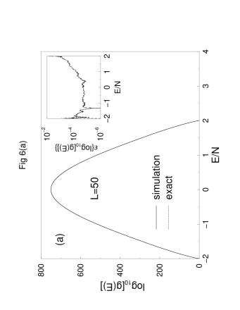
With the exact solution for the partition function on finite-size systems [40], and expansion of the expression by Mathematica, the density of states for the 2D Ising model on a square lattice can be obtained exactly [10]. Beale [10] obtained the exact density of states up to ; and because of the memory and speed limitation of present computers, we could only extend the calculation up to with the Mathematica program provided by Beale. With the algorithm proposed in this paper, the density of states for the Ising model is estimated for . The final modification factor for our random walk was for . In Fig. 6(a) the simulational densities of states are compared with exact results. With the logarithmic scale used in the figure simulational data and exact solution overlap perfectly with each other for . In the inset of the figure, we show the relative error , which is generally defined by the ratio between error of the simulational data and exact values for any quantity :
| (13) |
for most of the region is smaller than 0.1%. Such errors for low energy levels are directly related to the errors for the thermodynamic quantities calculated from the density of states. The average relative error is 0.019% for . It is possible to estimate the density of states for small systems with the broad histogram method [21, 22, 23]. Recent broad histogram simulational data [29] for the 2D Ising model on a lattice with MC sweeps yielded an average deviation of the microcanonical entropy of about 0.08 % from the exact solution [10]. With our algorithm we obtain an average error as small as 0.035 % on the lattice with MC sweeps. Procedures for allowing have been examined by Hüller [41] who used data from two densities of states for two different values of to extrapolate to . However, his data for a small Ising system yield larger errors than our direct approach. The applicability of his method to large systems also needs a more detailed study.
The absolute density of states in Fig. 6(a) is obtained by the condition that the number of ground states is 2 for the 2D Ising model (all up or down). This condition guarantees the accuracy of the density of states at low energy levels which are very important in the calculation of thermodynamic quantities at low temperature. With this condition, when , we can get exact solutions for internal energy, entropy and free energy when we calculate such quantities from the density of states. If we apply the condition that the total number of states is for the ferromagnetic Ising model, we can not guarantee the accuracy of the energy levels at or near ground states because the rescaled factor is dominated by the maximum density of states.
In Fig. 6(b), we show our estimation of the density of states of Ising model on lattice. Since the density of states for has almost no contribution to the canonical average at finite positive temperature, we only estimate the density of states in the region out of the whole energy . To speed up our calculation, we divide the desired energy region [-2, 0.2] into 15 energy segments, and estimate the density of states for each segment with independent random walks. The modification factor changes from to . The resultant density of states can be joined from adjacent energy segments. To reduce the boundary effects of the random walk on each segments, we keep about several hundred overlapping energy levels for random walks on two adjacent energy segments. The histograms of random walks are shown in the inset of this figure. We only require a flat histogram for each energy segment. To reduce the error of the density of states relevant to the accuracy of the thermodynamic quantities near we optimize the parameter and perform additional multiple random walks for the energy range with same number of processors. For this we use the density of states obtained from the first simulations as starting points and continue the random walk with modification factors changing from to . The total computational effort is about visits on each energy levels. Note that the total number of possible energy levels is and we perform random walks only on [-2, 0.2] out of [-2, 2]. The real simulational effort is about MC sweeps for the Ising model with . With the program we implemented, it took about 240 CPU hours on a single IBM SP Power3 processor.
For , we perform multiple random walks on different energy ranges, and one problem arises, that is the error of the density of states due to the random walk in a restricted energy range. Since the exact density of states for large systems is not available, we use to study such effects. We perform three independent random walks in the ranges , and to calculate the densities of states on these ranges. In Fig. 7(a), we show the errors of our simulation results from the exact values. We make our simulational densities of states match up with the exact results at the left edges. It is very clear that the width of the energy range of the random walks is almost not relevant to the errors of the density of states. The reason is that the random walks only require the local histogram to be flat as we discussed in the previous section. But the errors for the last two densities on the right edges are significantly larger than the others. The problem is the boundary effect because in this simulation we treat the densities of states at edges as same as those away from edges. That is not correct. Another reason is due to the flat histogram and high density at right side edges. Our simulational effort for the densities at the right edges is not enough compared to those at the left side. This is also the reason why we have not seen big errors at left edges.
To study the influence of the errors of the densities of states on the thermodynamic quantities calculated from them, in the energy range that we perform random walks, we replace the exact density of states with the simulational density of states. In Fig. 7(b), the specific heat calculated from such density of states is showed as a function of temperature. We also show the exact value with the simulational data, the difference is obvious.
To reduce the boundary effect, we delete the last two density entries, and insert them into the exact density of states again, then the results in Fig. 7(c) are much better.
With our test in the three different ranges of energy, it is quite safe to conclude that boundary effect will not be present in our multiply random walks if we have a couple of energy levels overlap for adjacent energy ranges. In our real simulations for large systems, we have hundreds of overlaping energy levels.
Since the exact density of states is only available on small systems (), it is not so interesting to compare the simulational density of states itself. The most important thing is the accuracy of estimations of thermodynamic quantities calculated from such density of states on large systems. With the density of states on large systems, we apply canonical average formulas to calculate internal energy, specific heat, Gibbs free energy and entropy. Ferdinand and Fisher [40] obtained the exact solutions of above quantities for 2D Ising model on finite-size lattices. Our simulational results on finite-size lattice can be compared with those exact solutions.
In Fig. 8(a), we show the internal energy as a function of temperature. The internal energy is estimated from the canonical average over energy of the system as the equation (7). We also draw the exact solution in the same graph. The exact and simulational data perfectly overlap with each other in a wide temperature region from to . Since no difference is visible with the scale used in Fig. 8(a), a more stringent test of the accuracy is provided by the inset which shows the relative errors . With the density of states obtained with our algorithm, the relative error of simulational internal energy for is smaller than 0.09% for the temperature region from to . From eqn. (7) it is very clear that the canonical distribution serves as a weighting factor, and since the distribution is very narrow, is only determined by a small portion of the density of states. (For the 2D Ising model at , only the density of states for contributes in a major way to the calculation.) Therefore the error is also determined by the errors of the density of states in the same narrow energy range.
With the density of states and equation (8), we also can calculate the specific heat per lattice site as a function of temperature. Both simulational data and exact results near are shown in Fig. 8(b) for , 128 and 256 Ising model in the vicinity of . Within the resolution of the figure, we can see the difference between the simulational data and exact solutions. In the inset of Fig. 8(b), we present relative errors for our simulational data as a function of temperature for . The errors for the specific heat for the Ising model on a lattice are smaller than in all temperature region . Very recently, Wang, Tay and Swendsen [38] estimated the specific heat of the same model on a lattice by the transition matrix Monte Carlo re-weighting method [42], and for a simulation with MC sweeps, the maximum error in temperature region was about 1%. When we apply our algorithm to the same model on the lattice, with a final modification factor of and a total of MC sweeps on single processor, the errors in the specific heat are reduced below 0.7% for all temperatures. The relatively large errors at low temperature reflect the small values for the specific heat at low temperature. According to the simulational data by broad histogram method, the errors in specific heat are very large even for systems as small as [21, 22, 23]. Only very recently, they have reduced the error near to a small value for [43].
In Fig. 8(c), the free energy for is plotted as a function of temperature. For comparison the exact solution [40] is shown in the same figure. As expected, simulational and exact data overlap perfectly within the resolution of the figure. Since the system has a second-order phase transition, unlike the Potts model, the first derivative of the free energy is a continuous function of temperature. The result very close to is shown in the inset of Fig. 8(c) for . The behavior of the free energy near is quite different from that of the first-order phase transition in Fig. 4(c). According to our calculation, the relative errors for all temperatures from to are smaller than 0.0008%, which means that our simulational data agree almost perfectly with the exact solution [30]. Since we use the condition that the number of ground states is to normalize the density of states, the errors at low temperatures are extremely small.
The entropy of the 2D Ising model can be calculated with the equation(12). In Fig. 8(d), the simulational data and exact results are presented in the same figure. With the scale in the figure, the difference between our simulational data and exact solutions are not visible. In the inset of Fig. 8(d), the relative errors of our simulational data are plotted as a function of temperature. For the Ising model on a lattice, the relative errors are smaller than 1.2% for all temperature range. We also notice that the errors near decrease dramatically. The reason is the condition we use to normalize the density of states. Very recently, with the flat histogram method [28] and the broad histogram method [21, 22, 23], the entropy was estimated with MC sweeps for the same model on lattice; however, the errors in reference [24] are even much bigger than our errors for !
V Application to 3D EA model
Spin glasses [44] are magnetic systems in which the interactions between the magnetic moments produce frustration because of some structural disorder. One of the simplest theoretical models for such systems is the Edwards-Anderson model [45] (EA model) proposed twenty five years ago. For such disordered systems, analytical methods can provide only very limited information, so computer simulations play a particularly important role. However, because of the rough energy landscape of such disordered systems, the relaxation times of the conventional Monte Carlo simulations are very long. The dynamical critical exponent was estimated as large as [46, 47, 48]. Normally simulations can be performed only on rather small systems, and many properties concerning the spin glasses are still left unclarified [49, 50, 51, 52, 53, 54, 55, 56].
In this paper, we consider the three-dimensional Ising spin glass EA model. The model is defined by the Hamiltonian
| (14) |
where is an Ising spin and the coupling is quenched to randomly. The summation runs over the nearest-neighbors on a simple cubic lattice.
One of most important issues for a spin glass model is the low temperature behavior. Because of the slow dynamics and rough phase space landscape of this model, it is also one of most difficult problems in simulational physics. The algorithm proposed here is not only very efficient in estimating the density of states but also very aggressive in finding the ground states. From a random walk in energy space, we can estimate the ground state energy and the density of states very easily. For a spin glass system, after we finish the random walk, we can obtain the absolute density of states by the condition that total number of states is . The entropy at zero temperature can be calculated from either or , where is the energy at ground states. Both relations will give the same result since and are calculated from the same density of states. Our estimates for and per lattice site, listed in Table 2, agree with the corresponding estimates made with the multicanonical method. With our algorithm, we can estimate the density of states up to by a random walk in energy space for few hours on a 400MHz processor.
If we are only interested in the quantities directly related to the energy, such as free energy, entropy, internal energy and specific heat, one dimensional random walk in energy space will allow us to calculate these quantities with a high accuracy as we did in the 2D Ising model. However for spin glass systems, one of the most important quantities is the order parameter which can be defined by [45]
| (15) |
Here, is the total number of the spins in the system, is the linear size of the system, is the auto-correlation function, which depends on the temperature and the evolution time , and . When , becomes the order parameter of the spin glass. This parameter takes the following values
| (16) |
The value at can be different from 1 in the case where the ground state is highly degenerate.
In our simulation, there is no temperature introduced during the random walk. And it is more efficient to perform a random walk in single system than two replicas. So the order-parameter can be defined
| (17) |
where is one of spin configurations at ground states and is any configuration during the random walk. The behavior of we defined above is basically the same as the order-parameter defined by the Edwards and Anderson [45]. It is not exact same order-parameter defined by Edwards and Anderson, but was used in the early numerical simulations by Binder et al.[57, 58].
After first generating a bond configuration we perform a one-dimensional random walk in energy space to find a spin configuration for the ground states. Since the order-parameter is not directly related to the energy, to get a good estimate of this quantity we have to perform a two-dimensional random walk to obtain the density of states with a flat histogram in - space. This also allows us to overcome the barriers in parameter space (or configuration space) for such a complex system. The rule for the 2D random walk is the same as 1D random walk in the energy space.
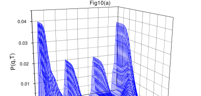
In Fig. 9, we show the histogram of the 2D random walk in energy-order parameter space, which is very flat. With the density of states , we can calculate any quantities as we did in the previous sections. It is very interesting to study the roughness of this model. First we study the canonical distribution as a function of the order-parameter:
| (18) |
In Fig. 10(a), we show a 3D plot for the canonical distribution at different temperatures for one bond configuration of EA model. At low temperatures, there are four peaks, and the depth of the valleys between peaks depends upon temperature. When the temperature is high, the multiple peaks converge to a single central peak. Because we use the linear scale to show our result in the Fig. 10(a). It is not clear how deep the dips among peaks are. In Fig. 10(b), we show the canonical distribution using logarithmic scale for the same distribution but only at , and we find that the dips are as deep as . We also noted there actually are six peaks, but the plot with linear scale does not show all of them because two are as small as compared to other four peaks.
In Fig. 11(a), we show the roughness of the canonical distribution for another realization on an lattice. Because of the wide variation in the distribution at low temperature we used a logarithmic scale: the relative size of dips are as deep as at . There are several local minima even at high temperatures. With conventional Monte Carlo simulations, it is almost impossible to overcome the barriers at the low temperature, so the simulation will get trapped in one of the local minima as shown in the figure. With our algorithm all states will be visited with more or less the same probability and trapping is not a problem.
With the density of states , we also can calculate the energy landscape by:
| (19) |
In Fig. 11(b), we show the internal energy as a function of order-parameter for temperatures . We find that the landscape is a very rough at low temperatures. The roughness of the energy landscape agrees with the one for canonical distribution. But the maxima in energy landscape are corresponding to the minima approximately in the canonical distribution.
As we already noted in the previous paragraph, the roughness of the landscape of the spin glass model makes the conventional Monte Carlo simulation extremely difficult to apply. Therefore, even a quarter of a century after the model was proposed, we even can not conclude whether there is a finite phase transition between glass phase and disordered phase. With Monte Carlo simulations on a large system () and a finite-size scaling analysis on a small lattice, Marinari et al. [59] expressed doubt about the existence of the “well-established” finite-temperature phase transition of the 3D Ising spin glass [46, 49]. Their simulational data can be described equally well by a finite-temperature transition or by a singularity of an unusual type. Kawashima and Young’s simulational data could also not rule out the possibility of [50]. Thus even the existence of the finite-temperature phase transition is still controversial, and thus the nature of the spin glass state is uncertain. Although the best available computer simulation results [15, 54, 60] have been interpreted as a mean-field like behavior with replica-symmetry breaking(RSB) [61], Moore et al. showed evidence for the droplet picture [62] of spin glasses within the Migdal-Kadanoff approximation. They argued that the failure to see droplet model behavior in Monte Carlo simulations was due to the fact that all existing simulations are done at temperatures too close to transition temperature so that system sizes larger than the correlation length were not used. As discussed in the previous paragraph, the lower the temperature is, the rougher the canonical distribution and energy landscape are; hence, it is almost impossible for conventional Monte Carlo methods to overcome the barrier between local minima and globe minima. It is possible to heat the system up to increase the possibility of escape from local minima by simulated annealing and the more recent simulated tempering method [63] and parallel tempering method [64, 65], but it is still very difficult to perform equilibrium simulations at low temperatures. Very recently Hatano and Gubernatis proposed a bivariate multicanonical Monte Carlo method for the 3D spin glass model, and their result also favors the droplet picture [18, 66]. Marinari, Parisi et al. argued, however, that the data were not thermalized [60]. The nature of spin glasses thus remains controversial [53].
The algorithm proposed in this paper provides an alternative for the study of complex systems. Because we need to calculate the order-parameter with high accuracy, and this quantity is not directly related to the energy, we need to perform a random walk in the two-dimensional energy - order parameter space. After we estimate the density of states in this space, we can calculate the order-parameter at any temperature from the canonical average. In 12(a), we show our results for the EA model for , 6 and 8. Because we need to perform a 2D random walk with a total of about states, the simulation is only a practical for a small system(). The results in the figure are the average over 100 realizations for , 50 realizations for and 20 for .
We notice that the behavior of is very similar to the magnetization (the order-parameter for the Ising model), but the finite value at low temperature is not necessarily equal to 1 because of the high degeneracy of the ground state for the spin glass model. The fluctuation of the order-parameter at the different temperatures for , 6 and 8 is shown in the inset of the figure.
To estimate the transition temperature of the spin glass system, we calculated the fourth order cumulant as a function of temperature. In Fig. 12(b), we show our simulational results for , 6 and 8. All curves clearly cross around . Below this temperature, the spin configurations are frozen into some disorder ground states and the order parameter assumes a finite value. Above this temperature , the system is in a disordered states and the order parameter vanishes.
One complication for simulation of such random systems is the determination of the relative importance of the error due to the simulation algorithm and the error due to the finite sampling of bond distributions. From Fig. 12 (a) and (b), we can not tell what the origin of the error bars is so we also performed multiple independent simulations for the same bond configuration on a 3D EA model. We found that the statistical errors for the order parameter and the fourth order cumulant from these simulations were much smaller than the error bars shown in Fig. 12 (a) and (b) for all temperatures. We conclude that the error bars in the figure arise almost completely from the randomness of the system.
The computational resources devoted here to the EA model were not immense. All our simulations for one bond configuration (, 6 and 8) were performed within two days on (multiple) Linux machines (MHz) in the Center for Simulational Physics. This effort should thus be viewed as a feasibility study, and substantially more effort would be required to determine the nature of the spin glass phase or to estimate the transition temperature with high accuracy. Nonetheless, we believe that these results show the applicability of our method to systems with a rough landscape. Because of the number of states is about for random walks, such calculations not only require huge memory during the simulation but also substantial disk space to store the density of states for the later calculation of thermodynamic quantities.
VI Discussion and Conclusion
In this paper, we proposed an efficient algorithm to calculate the density of states directly for large systems. By modifying the estimate at each step of the random walk in energy space and carefully controlling the modification factor, we can determine the density of states very accurately. Using the density of states, we can then calculate thermodynamic quantities at essentially any temperature by applying simple statistical physics formulas. An important advantage of this approach is that we can also calculate the Gibbs free energy and entropy, quantities that are not directly available from conventional Monte Carlo simulations.
We applied our method to the Potts model which demonstrates a typical first-order phase transition. By estimating the density of states with lattices as large as , we calculated the internal energy, specific heat, free energy and entropy in a wide temperature region. We found a typical first-order phase transition with a “discontinuity” for the internal energy and entropy at . The first derivative of the free energy also shows such a discontinuity at . The transition temperature estimated from simulational data is consistent with the exact solution.
We also applied our algorithm to the Ising model, which shows a second-order phase transition. The density of states obtained by the end of our simulations was compared directly with the exact solution on lattice. The relative errors for most important energy levels are less than 0.019%. It was also possible to calculate the density of states for a lattice with a computational effort of Monte Carlo sweeps. With the accurate density of states, we calculated the internal energy, specific heat, Gibbs free energy and entropy. For all temperatures between and , the relative errors are smaller than for internal energy, for free energy, for entropy and for specific heat.
We should point out that our simulational results for are close to the same accuracy as the specific heat of the Ising model for with the transition matrix Monte Carlo re-weighting method with MC sweeps [38]. Our estimate of the entropy for the 2D Ising model for the lattice is even more accurate than the results obtained for the same quantity for with the broad histogram method and flat histogram method [24], which needed about MC sweeps. Our simulational effort for was MC sweeps.
The algorithm was also applied with success to the EA spin glass model for which we could determine the roughness of the energy landscape and canonical distribution in order-parameter space. The internal energy and entropy at zero temperature were estimated up to a lattice size , and the transition temperature was estimated as about .
In this paper, we only concentrated the random walk in energy space (and order-parameter space); however, the idea is very general and we can apply this algorithm to any parameters [13]. The energy levels of the models treated here are perfectly discrete and the total number of possible energy levels is known before simulation, but in a general model such information is not available. Since the histogram of the random walk with our algorithm tends to be flat, it is very easy to probe all possible energies and monitor the histogram entry at each energy level. For some models where all possible energy levels can not be fitted in the computer memory or the energy is continuous, e.g. the Heisenberg model, we may need to discretize the energy levels. According our experience on discrete and continuous models, if the total number of possible energies is around the number of lattice sites , the algorithm is very efficient for studying both first- or second-order phase transitions.
In this paper, we only applied our algorithm to simple models, but since the algorithm is very efficient even for large systems it should be very useful in the studies of general, complex systems with rough landscapes. It is clear, however, that more investigation is needed to better determine under which circumstances our method offers substantial advantage over other approaches and we wish to encourage the application of this approach to other models.
ACKNOWLEDGMENTS
We would like to thank S. P. Lewis, H-B Schuttler, T. Neuhaus and A. Hüller for comments and suggestions, K. Binder, N. Hatano, P. M. C. de Oliveira and C. K. Hu for helpful discussions. We also thank M. Caplinger for support on technical matters and P. D. Beale for providing his Mathematica program for the calculation of the exact density of states for the Ising model. The research project is supported by the National Science Foundation under Grant No. DMR-0094422.
REFERENCES
- [1] D. P. Landau and K. Binder, A Guide to Monte Carlo Methods in Statistical Physics, (Cambridge U. Press, Cambridge, 2000).
- [2] N. Metropolis, A. W. Rosenbluth, M. N. Rosenbluth, A. M. Teller and E. Teller, J. Chem. Phys. 21, 1087, (1953).
- [3] R. H. Swendsen and J.-S. Wang, Phys. Rev. Lett. 58, 86 (1987).
- [4] U. Wolff, Phys. Rev. Lett. 62, 361 (1989).
- [5] B. A. Berg and T. Neuhaus, Phys. Rev. Lett. 68, 9 (1992).
- [6] W. Janke and S. Kappler, Phys. Rev. Lett. 74, 212 (1995).
- [7] B. A. Berg and T. Celik, Phys. Rev. Lett. 69, 2292 (1992).
- [8] N. S. Alves and U. Hansmann, Phys. Rev. Lett. 84, 1836 (2000).
- [9] A. M. Ferrenberg and R. H. Swendsen, Phys. Rev. Lett. 61, 2635 (1988), 63, 1195 (1989).
- [10] P. D. Beale, Phys. Rev. Lett. 76, 78 (1996).
- [11] B. A. Berg and T. Neuhaus, Phys. Lett. B 267, 249 (1991).
- [12] W. Janke, Int. J. Mod. Phys. C 3, 375 (1992).
- [13] B. A. Berg and U. Hansmann and T. Neuhaus, Phys. Rev. B 47, 497 (1993).
- [14] W. Janke, Physica A 254, 164 (1998).
- [15] B. A. Berg and W. Janke, Phys. Rev. Lett. 80, 4771 (1998).
- [16] B. A. Berg, Nucl. Phys. B, 63, 982 (1998).
- [17] B. A. Berg T. Celik and U. Hansmann, Eur. Phys. Lett. 22, 63 (1993).
- [18] N. Hatano and J. E. Gubernatis in Computer Simulation Studies in Condensed Matter Physics XII, D. P. Landau, S. P. Lewis and H.-B. Schuttler (eds) (Springer, Berlin, Heidelberg, 2000).
- [19] B. A. Berg J. Stat. Phys. 82, 323 (1996).
- [20] J. Lee, Phys. Rev. Lett. 71, 211 (1993).
- [21] P. M. C. de Oliveira, T. J. P. Penna and H. J. Herrmann, Braz. J. Phys. 26, 677 (1996).
- [22] P. M. C. de Oliveira, T. J. P. Penna and H. J. Herrmann, Eur. Phys. J. B. 1, 205 (1998).
- [23] P. M. C. de Oliveira, Eur. Phys. J. B. 6, 111 (1998).
- [24] J. S. Wang and L W Lee, Comput. Phys. Commun. 127, 131, (2000).
- [25] P. M. C. de Oliveira, private communication.
- [26] J. S. Wang, Cond-matt-9909177.
- [27] B. A. Berg and U. Hansmann, Eur. Phys. J. B 6, 395 (1998).
- [28] J. S. Wang, Eur. Phys. J. B. 8, 287 (1998).
- [29] A. R. Lima, P. M. C. de Oliveira and T. J. P. Penna, J. Stat. Phys. 99, 691, (2000).
- [30] F. Wang and D. P. Landau, Phys. Rev. Lett. 86, 2050 (2001).
- [31] U. Hansmann, Phys. Rev. B 56, 6200 (1997).
- [32] U. Hansmann and Y. Okamoto, Phys. Rev. E 54, 5863 (1996).
- [33] W. Janke, B. A. Berg and A. Billoire, Comp. Phys. Commun. 121-122, 176 (1999).
- [34] F. Y. Wu, Rev. Mod. Phys. 54, 235 (1982).
- [35] K. Binder, K. Vollmayr, H. P. Deutsch, J. D. Reger M. Scheucher and D. P. Landau, Int. J. of Mod. Phys. C 5, 1025, (1992).
- [36] M. S. S. Challa, D. P. Landau and K. Binder Phys. Rev. B 34, 1841, (1986).
- [37] T. Neuhaus, private communication
- [38] J. S. Wang, T. K. Tay and R. H. Swendsen, Phys. Rev. Lett. 82, 476 (1999).
- [39] D. P. Landau, Phys Rev. B 13, 2997 (1976).
- [40] A. E. Ferdinand and M. E. Fisher, Phys. Rev. 185, 832 (1969).
- [41] A. Hüller Cond-mat/0011379
- [42] R. H. Swendsen, J. S. Wang, S. T Li, B. Diggs, C. Genovese and J. B. Kadane, Int. J. of Mod. Phys. C 10, 1563 (1999).
- [43] P. M. C. de Oliveira, Braz. J. Phys. 30, 4659 (2000).
- [44] K. Binder and A.P. Young, Rev. Mod. Phys. 58, 801 (1986).
- [45] S.F. Edwards and P.W. Anderson, J Phys. F. Metal Phys. 5, 965 (1975).
- [46] A.T. Ogielski and I. Morgenstern, Phys. Rev. Lett. 54, 928 (1985).
- [47] F. Wang, N. Kawashima and M. Suzuki, Europhys. Lett. 33, 165 (1996).
- [48] F. Wang, N. Kawashima and M. Suzuki, Int. J. Mod. Phys. C 7, 573 (1996).
- [49] R.N. Bhatt and A.P. Young, Phys. Rev. Lett. 54, 924 (1985).
- [50] N. Kawashima and A.P. Young, Phys. Rev. B 53, R484 (1996).
- [51] M. Palassini and A. P. Young, Phys. Rev. Lett. 82, 5128 (1999).
- [52] M. Palassini and A. P. Young, Phys. Rev. Lett. 83, 5126 (1999).
- [53] M. Palassini and A. P. Young, Phys. Rev. Lett. 85, 3017 (2000).
- [54] E. Marinari, Phys. Rev. Lett. 82, 434 (1999).
- [55] M. A. Moore, H. Bokil and B. Drossel, Phys. Rev. Lett. 81, 4252 (1999).
- [56] J. Houdayer and O. C. Martin, Phys. Rev. Lett. 82, 4934 (1999).
- [57] I. Morgenstern and K. Binder, Phys. Rev. B22, 288 (1980).
- [58] K. Binder in Fundamental problems in statistical mechanics V, edited by E. G. D. Cohen, (North-Holland, 1980).
- [59] E. Marinari, G. Parisi and F. Ritort, J. Phys. A 27 2687 (1994).
- [60] E. Marinari, G. Parisi, F. Ricci-Tersenghi and F. Zuliani, Cond-mat/0011039
- [61] G. Parisi, Phys. Rev. Lett. 43, 1754 (1979), 50, 1946 (1983).
- [62] D. S. Fisher and D. A. Huse, Phys. Rev. B 38, 386 (1988).
- [63] E. Marinari and G. Parisi, Europhys. Lett. 19, 451 (1992).
- [64] K. Hukushima and K. Nemoto, J. Phys. Soc. Japan 65, 1604 (1996).
- [65] K. Hukushima, in Computer Simulation Studies in Condensed Matter Physics XIII, D. P. Landau, S. P. Lewis and H.-B. Schuttler (eds) (Springer, Berlin, Heidelberg, 2000).
- [66] N. Hatano and J. E. Gubernatis, Cond-mat/0008115

(a)

(b)


(a)

(b)

(c)

(d)

(a)

(b)

(a)
(b)

(a)

(b)

(c)

(a)

(b)

(c)

(d)


(a)
(b)

(a)

(b)

(a)

(b)

| size | Our method | MUCA | MUBO | ||||||
|---|---|---|---|---|---|---|---|---|---|
| L | |||||||||
| 12 | 0.70991 | 0.8402 | 1.7013 | 0.710540 | 0.806 | 1.688 | 0.7105402 | 0.833 | 1.72 |
| 16 | 0.70653 | 0.8694 | 1.6967 | 0.706544 | 0.844 | 1.676 | 0.7065144 | 0.867 | 1.71 |
| 20 | 0.70511 | 0.8925 | 1.6875 | 0.7047891 | 0.883 | 1.69 | |||
| 24 | 0.70362 | 0.8940 | 1.6765 | 0.703730 | 0.908 | 1.698 | |||
| 26 | 0.70317 | 0.9002 | 1.6805 | 0.7034120 | 0.908 | 1.682 | |||
| 30 | 0.70289 | 0.9233 | 1.6888 | ||||||
| 34 | 0.70258 | 0.9343 | 1.6732 | 0.702553 | 0.927 | 1.683 | 0.7025530 | 0.921 | 1.676 |
| 40 | 0.70239 | 0.9337 | 1.6731 | ||||||
| 50 | 0.70177 | 0.9416 | 1.6776 | 0.7018765 | 0.940 | 1.674 | |||
| 60 | 0.70171 | 0.9522 | 1.6733 | ||||||
| 70 | 0.70153 | 0.9519 | 1.6717 | 0.701562 | 0.9511 | 1.670 | |||
| 80 | 0.70143 | 0.9576 | 1.6701 | ||||||
| 90 | 0.70141 | 0.9551 | 1.6727 | ||||||
| 100 | 0.70135 | 0.9615 | 1.6699 | 0.701378 | 0.9594 | 1.6699 | |||
| 120 | 0.70131 | 0.9803 | 1.6543 | ||||||
| 150 | 0.70127 | 0.9674 | 1.6738 | ||||||
| 200 | 0.70124 | 0.9647 | 1.6710 | ||||||
| exact | 0.701232… |
| size | Our Method | MUCA | ||
|---|---|---|---|---|
| L | ||||
| 4 | ||||
| 6 | ||||
| 8 | ||||
| 12 | ||||
| 16 | ||||
| 20 |