On the choice of the density matrix
in the stochastic TMRG

Abstract

In applications of the density matrix renormalization group to nonhermitean problems, the choice of the density matrix is not uniquely prescribed by the algorithm. We demonstrate that for the recently introduced stochastic transfer matrix DMRG (stochastic TMRG) the necessity to use open boundary conditions makes asymmetrical reduced density matrices, as used for renormalization in quantum TMRG, an inappropriate choice. An explicit construction of the largest left and right eigenvectors of the full transfer matrix allows us to show why symmetrical density matrices are the correct physical choice.

,

1 Introduction

Since its inception in 1992 by White[1], the Density Matrix Renormalization Group (DMRG) has emerged as one of the most powerful numerical methods in the study of low dimensional strongly correlated fermionic, bosonic or quantum magnetic systems[2]. The universality of its core idea of deducing a decimation prescription for state spaces by considering the renormalization flow of suitable reduced density matrices has led many researchers to extend the method to other fields of research in systems with many correlated degrees of freedom.

Originally, the method was applied to the renormalization of effective low-energy Hamiltonians to study static and dynamic $T=0$ properties. Major progress occurred with Nishino’s realisation[3] that the DMRG can be used to renormalize the transfer matrix of semi-infinite two-dimensional strips, a method which we will refer to as TMRG (transfer matrix renormalization group) in the following. The use of a transfer matrix implies that the system is truly infinite in one spatial direction, whereas the power of the DMRG to treat large one-dimensional systems is reflected in the fact that the strip width can be chosen so large as to allow reliable finite-size extrapolations. In analogy to the approach used in Quantum Monte Carlo, one-dimensional quantum systems were then mapped by a Trotter-Suzuki checkerboard decomposition to a two-dimensional classical system[4]. The renormalization of the resulting quantum transfer matrix allows the study of the thermodynamics of quantum chains for infinite system sizes and very fine Trotter-Suzuki decompositions, i.e. down to very low temperatures.

As the Trotter-Suzuki decomposition generates a transfer matrix which is not invariant under a spatial reflection of the system, the quantum transfer matrix is asymmetrical and there are left and right eigenstates $\langle\psi_{L}|$ and $|\psi_{R}\rangle$ associated with the thermodynamically relevant largest eigenvalue of the transfer matrix. This raises the question which is the correct way to construct the optimal density matrix for the DMRG. In the usual hermitean DMRG, the density matrix is typically obtained by tracing out a part of the universe (“environment”) in the ground state:

$$\rho_{\text{sys}}=\Tr_{\text{env}}|\psi\rangle\langle\psi|.$$ (1)

In the nonhermitean case, Bursill et al[4] made the symmetrical choice

$$\rho_{\text{sys}}=\Tr_{\text{env}}|\psi_{R}\rangle\langle\psi_{R}|$$ (2)

which can be easily extended to

$$\rho_{\text{sys}}^{\text{symm}}=\Tr_{\text{env}}(|\psi_{R}\rangle\langle\psi_{R}|+|\psi_{L}\rangle\langle\psi_{L}|)$$ (3)

which treats the left and right eigenvectors on an equal footing (all composite density matrices have to be appropriately normalized, depending on the normalization chosen for the eigenvectors; we do not show these factors explicitly in the paper). This approach also has the property to minimize the sum of the two squared distances between the original eigenstates and their projections onto the reduced state spaces after the renormalization step, which is the prescription from which the DMRG procedure for symmetrical matrices can be derived.

However, it was pointed out by Wang and Xiang[5] that the choice of an asymmetrical density matrix,

$$\rho_{\text{sys}}^{\text{asym}}=\Tr_{\text{env}}|\psi_{R}\rangle\langle\psi_{L}|,$$ (4)

is more physically adequate and yields numerically more satisfying results. This is now the accepted choice for the application of the TMRG to quantum problems[6, 7, 8].

A further field of applications was opened up by the application of the DMRG idea to the renormalization of genuinely asymmetrical problems[9, 10, 11] as they occur in nonequilibrium statistical mechanics. Carlon, Henkel and Schollwöck[11] exploited the fact that the time evolution of reaction-diffusion systems can be mapped to a Schrödinger-like equation. In this case, one can study the long-time behaviour of finite size systems quite precisely[11, 12, 13, 14].

Here, the question of the correct choice of the density matrix arises as the transition matrix is genuinely asymmetrical itself, since there is no detailed balance. Carlon et al found the choice of the symmetrical density matrix to be most suitable, but essentially due to reasons of numerical stability: in this class of problems, very high numerical precision for the chosen basis states in the reduced basis was found to be important, which is less easily obtained for asymmetrical matrices. An attempt to include projectors like $|\psi_{R}\rangle\langle\psi_{L}|$ while building a symmetrical density matrix by studying

$$\rho_{\text{sys}}^{\text{mix}}=\Tr_{\text{env}}(|\psi_{L}\rangle+|\psi_{R}\rangle)(\langle\psi_{L}|+\langle\psi_{R}|),$$ (5)

yielded inferior results.

Recently, the TMRG has been used by Kemper et al to successfully renormalize stochastic transfer matrices[15], an approach which henceforth we will refer to as “stochastic TMRG”. In their study of the Domany-Kinzel cellular automaton, they found that the use of a symmetrical density matrix yielded satisfactory results, while the asymmetrical choice led to incorrect results, which is at variance with the conventional (or “quantum”) TMRG. These findings were obtained on an entirely empirical basis.

In this paper, we want to investigate in depth the question of the correct choice of the density matrix, which is at the core of all asymmetrical DMRG applications, for the new stochastic TMRG. We will give explicit constructions for the eigenvalues and selected eigenvectors of the stochastic transfer matrices, highlighting the central role of the boundary conditions in time direction. This will allow us to demonstrate that the content of the asymmetrical density matrix is essentially trivial, while the symmetrical density matrix is the physically adequate choice.

2 Explicit construction of the unrenormalized TMRG transfer matrix

2.1 The TMRG transfer matrix

In the stochastic TMRG (for a description of the very similar TMRG applied to quantum systems, see [2]), one considers a stochastically evolving system extended infinitely in one spatial dimension with (for simplicity) local update rules involving neighbouring sites only that allow a finite number of states ($n$). The local interaction between two (or similarly, a few) lattice sites is given by the local transfer matrix

$$(\tau)_{l_{1}r_{1}}^{l_{2}r_{2}}=[\exp(\Delta t\cdot H_{\text{local}})]_{l_{1}r_{1}}^{l_{2}r_{2}}=\raisebox{-14.22636pt}{\includegraphics{tau2.eps}}$$ (6)

where the stochastic “Hamiltonian” $H_{\text{local}}$ gives the transition rates between states and the arrow indicates the direction of the time step $\Delta t$. We assume spatial parity invariance

$$(\tau)_{l_{1}r_{1}}^{l_{2}r_{2}}=(\tau)_{r_{1}l_{1}}^{r_{2}l_{2}}\,.$$ (7)

In complete analogy to Quantum Monte Carlo and the conventional TMRG, the real time evolution operator for the full lattice is mapped approximately by a Trotter-Suzuki decomposition to a checkerboard structure of local interactions (figure 1).

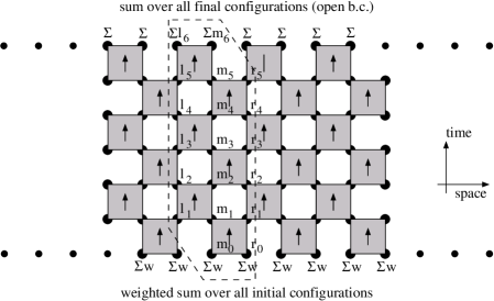
Figure 1: Trotter-Suzuki decomposition of the full time evolution into local interactions $\tau$ ($2M=6$ time steps shown). The lattice is spatially infinitely extended, while in time direction the system is finite. Two adjacent columns (boxed) constitute the basic building block: the transfer matrix $(T)^{l_{1}\dots l_{2M-1}}_{r_{1}\dots r_{2M-1}}$.

In the time direction the evolution of the system is simulated during a finite interval. As illustrated in figure 1, the full evolution operator is then written as $\exp(2M\Delta t\cdot H)=\lim_{N\to\infty}T^{N}$, where $M$ is the Trotter number, $N$ the (diverging) system size and $H=\lim_{N\rightarrow\infty}\sum_{i=-N}^{N}H_{\text{local}}(i,i+1)$. $T$ is called the transfer matrix which consists of two adjacent columns of $\tau$’s, where we take as upper (lower) index the “history” (time evolution) of the lattice site at the left (right) side of the zig-zagged column:

$$(T)^{l_{1}\dots l_{2M-1}}_{r_{1}\dots r_{2M-1}}=\underbrace{\sum_{m_{0}r_{0}}w(m_{0})\,w(r_{0})}_{\text{open initial b.c.}}\sum_{{m_{1}\dots\\ m_{2M-1}}}\underbrace{\sum_{l_{2M}m_{2M}}}_{\makebox[2.84526pt][c]{\scriptsize open final b.c.}}\prod_{k=0}^{M-1}(\tau)_{m_{2k}r_{2k}}^{m_{2k+1}r_{2k+1}}(\tau)_{l_{2k+1}m_{2k+1}}^{l_{2k+2}m_{2k+2}}$$ (8)

where $l$, $m$, and $r$ denote the left, middle and right lattice sites of $T$, respectively. One uses stochastic initial conditions: the weight of each possible initial configuration is given by the product of local weights $w(s_{i})$ of the states $s_{i}$ at each lattice site $i$,

$$w(\dots,s_{1},s_{2},s_{3},\dots)=\prod_{i}w(s_{i}),\qquad\sum_{s_{i}=1}^{n}w(s_{i})=1\text{ (norm.)}$$ (9)

such that if each state is weighted equally, there is no bias in the initial configuration. At the end, one uses open final boundary conditions, i.e. all final states are allowed without bias. In the diagrams, we thus implicitly trace over all internal indices, sum over all final indices, and perform a weighted sum over all initial indices.

2.2 Spectrum and eigenvectors of the transfer matrix

As the local stochastic transfer matrix $\tau$ must obey probability conservation, the probability of ending up in any state is unity:

$$\sum_{l_{2}r_{2}}(\tau)_{l_{1}r_{1}}^{l_{2}r_{2}}=1\quad\forall l_{1},r_{1},\qquad\raisebox{-14.22636pt}{\includegraphics{trivtau.eps}}\text{(trivial)}.$$ (10)

This implies

$$\Tr T=1,$$ (11)

where tracing contracts the upper index of $T$ with the lower one; thus the probability that the lattice sites at the left and right boundary of $T$ have the same time evolution is unity. In pictorial language, the trace rolls up the transfer matrix into a cylinder, with its left and right boundary identified and the middle site at the opposite side of the cylinder (cf. figure 2).

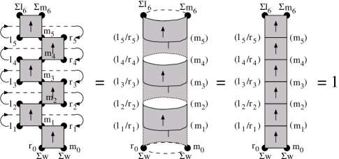
Figure 2: $\Tr(T)_{r_{1}\dots r_{2M-1}}^{l_{1}\dots l_{2M-1}}$ is equivalent to $T$ being rolled up on a cylinder with a solely local interaction.

But this is equivalent to having only the local interaction between the left/right lattice site on one side and the middle one on the other, for $2M$ time steps $\Delta t$, which is known exactly (e.g. $2M=6$):

$$(T)_{r_{1}\dots r_{5}}^{l_{1}\dots l_{5}}=\sum_{m_{0}r_{0}}w(m_{0})\,w(r_{0})\sum_{l_{6}m_{6}}\sum_{m_{1}\dots m_{5}}(\tau)_{l_{5}m_{5}}^{l_{6}m_{6}}(\tau)_{m_{4}r_{4}}^{m_{5}r_{5}}\cdots(\tau)_{l_{1}m_{1}}^{l_{2}m_{2}}(\tau)_{m_{0}r_{0}}^{m_{1}r_{1}}$$ (12)

$$\Tr T =\sum_{l_{1}\dots l_{5}}(T)_{l_{1}\dots l_{5}}^{l_{1}\dots l_{5}}$$

$$=\sum_{m_{0}r_{0}}w(m_{0})\,w(r_{0})\sum_{l_{6}m_{6}}\sum_{l_{1}\dots l_{5}}\sum_{m_{1}\dots m_{5}}(\tau)_{l_{5}m_{5}}^{l_{6}m_{6}}(\tau)_{m_{4}l_{4}}^{m_{5}l_{5}}\cdots(\tau)_{m_{0}l_{0}}^{m_{1}l_{1}}$$

$$=\sum_{m_{0}r_{0}}w(m_{0})\,w(r_{0})\sum_{l_{6}m_{6}}\left[\tau^{2M}(\Delta t)\right]_{r_{0}m_{0}}^{l_{6}m_{6}}\quad\text{(by parity invar.\ (\ref{eq:parity}))}$$

$$=\sum_{m_{0}r_{0}}w(m_{0})\,w(r_{0})\sum_{l_{6}m_{6}}\left[\exp(2M\Delta t\cdot H_{\text{local}})\right]_{r_{0}m_{0}}^{l_{6}m_{6}}$$

$$=\sum_{m_{0}r_{0}}w(m_{0})\,w(r_{0})\sum_{l_{6}m_{6}}\bigl{[}\tau(2M\Delta t)\bigr{]}_{r_{0}m_{0}}^{l_{6}m_{6}}$$

$$=\sum_{m_{0}r_{0}}w(m_{0})\,w(r_{0})\cdot 1=1\quad\text{(by (\ref{eq:sumtau}) and (\ref{eq:normw}))}.$$

Next we consider the spectrum and eigenvector decomposition of $T$. As all entries of $T$ are non-negative, the Frobenius theorem implies that the largest eigenvalue $\lambda_{0}$ is non-degenerate and real. The associated left and right eigenvectors $\langle\psi_{L}|$ and $|\psi_{R}\rangle$ (where $|\psi_{R}\rangle^{\dagger}\neq\langle\psi_{L}|$ in general, since $T$ is not symmetrical) have nonnegative entries. Now the decisive difference between conventional and stochastic TMRG is that in the conventional TMRG one has periodic boundary conditions in (imaginary) time, but open final boundary conditions in the stochastic TMRG. This latter property implies

$$T^{2M-1}=|\psi_{R}\rangle\langle\psi_{L}|=T^{k}\quad\forall k\geq 2M-1\,,$$ (13)

i.e. sufficiently large powers of $T$ are identical and decompose into an outer product of the two eigenvectors of $\lambda_{0}=1$, normalized as $\langle\psi_{L}|\psi_{R}\rangle=1$, while all other eigenvalues of $T$ vanish.

Figure 3: Open b.c. lead to trivial $\tau$’s that cause also the final indices of the previous $\tau$’s to be summed over, thus “propagating” the open b.c. backwards in time.

To see this, consider figure 3. Because $\tau$ is stochastic, it becomes trivial by summing over its final indices (cf. (10); its value does not depend on its initial indices, such that the contraction with the final index of a previous $\tau$ yields an unweighted sum over the previous $\tau$’s final index. Therefore in figure 4, the trivial $\tau$’s “propagate” the open final b.c. backwards in time, resulting in a cone of trivial $\tau$’s that have no influence on the value of the transfer matrix $T^{k}$.

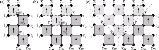
Figure 4: $T^{k}$ decompose into a left and right part of ever smaller rank until $T^{2M-1}$ decomposes into two lightcones which cannot interact during $2M$ time steps (here $2M=4$): (a) $T=(\psi_{R})_{m_{1}m_{2}}^{l_{1}l_{2}l_{3}}\cdot(\psi_{L})_{r_{1}r_{2}r_{3}}^{m_{1}m_{2}}$ with 2 connecting indices $(m_{1},m_{2})$, (b) $T^{2}=(\psi_{R})_{m_{1}}^{l_{1}l_{2}l_{3}}\cdot(\psi_{L})_{r_{1}r_{2}r_{3}}^{m_{1}}$ with one connecting index $(m_{1})$, (c) $T^{2M-1}=(\psi_{R})^{l_{1}l_{2}l_{3}}\cdot(\psi_{L})_{r_{1}r_{2}r_{3}}=|\psi_{R}\rangle\langle\psi_{L}|$ with no connecting index.

The Trotter-Suzuki decomposition introduces a finite speed of action (“speed of light”) into the model: during each time step, only nearest neighbours that are connected by an edge of a (nontrivial) $\tau$ can interact, so interactions can only propagate at a speed of one lattice site per time step $\Delta t$. Hence we speak of the “light cone” of a certain site as those sites in time and space that influence the probabilities of different occupations for this site.

In $T$ (cf. figure 4a), the last $\tau$ is trivial, hence it has the value 1 indepedent of $l_{3}$ and $m_{3}$. Thus we effectively sum over the internal index $m_{3}$, and $l_{3}$ is a “dummy index”: the value of $(T)_{r_{1}r_{2}r_{3}}^{l_{1}l_{2}l_{3}}$ does not depend on it. This leaves only two indices $(m_{1},m_{2})$ connecting the left and right part of $T$, so the transfer matrix can be decomposed into a product of two matrices $\psi_{R}$ and $\psi_{L}$ of rank $n^{2}$ ($n$ is the number of possible states per site).

When we multiply this with another $T$ (cf. figure 4b), we observe that a third $\tau$ becomes trivial as the final $\tau$’s propagate the final open b.c. backwards. This leads to a sum also over $m_{2}$, leaving $m_{1}$ as the only connecting index, so $T^{2}$ decomposes into a product of two matrices of rank $n$.

Finally in $T^{2M-1}$ (cf. figure 4c), the trivial $\tau$’s propagate all the way to the initial $\tau$’s, effectively separating the left and right boundary: now there are no connecting indices left between $\psi_{R}$ and $\psi_{L}$, turning them into column and row vectors $|\psi_{R}\rangle$ and $\langle\psi_{L}|$. From the viewpoint of causality, the left and right boundary are separated by $4M-2$ lattice sites, so no initial lattice site can influence both the left and the right boundary, i.e. the light cone for the lattice sites on the left boundary ($l_{1},\dots,l_{2M-1}$) does not intersect the light cone for the lattice sites on the right boundary ($r_{1},\dots,r_{2M-1}$). This means that the probability of a particular history on the left boundary is completely independent of the probability of a particular history on the right.

We can now explicitly compute these column and row vectors $|\psi_{R}\rangle^{l_{1}\dots l_{2M-1}}$ and $\langle\psi_{L}|_{r_{1}\dots r_{2M-1}}$: we take the left light cone (of triangular shape, delimited by the dashed line) and contract the included nontrivial local transfer matrices $\tau$ in all internal, initial, and final indices, keeping the free indices $l_{1}\dots l_{2M-1}$, and denote this object as (right eigenvector, see below) $|\psi_{R}\rangle^{l_{1}\dots l_{2M-1}}$. Analogously, we denote the same construction on the right with free indices $r_{1}\dots r_{2M-1}$ as $\langle\psi_{L}|_{r_{1}\dots r_{2M-1}}$. Note that the last index on the left, $l_{2M-1}$, is by construction a dummy index which does not change the value of $|\psi_{R}\rangle^{l_{1}\dots l_{2M-1}}$.

If we consider even higher powers of $T$ than $2M-1$, we only add more trivial $\tau$’s in the middle that lie outside either light cone and therefore do not change the value of the transfer matrix. Thus we have proven $T^{2M-1}=T^{k}\;\forall k\geq 2M-1$, which implies for the eigenvalues $\lambda_{i}$ of $T$ that $\lambda_{i}^{2M-1}=\lambda_{i}^{2M}\;\forall i$, such that $\lambda_{i}$ can only assume the values 0 or 1. From (11) follows $\lambda_{0}=1$, $\lambda_{i}=0\;\forall i>0$.

The above decomposition of $T^{2M-1}$ into an outer product of two vectors $|\psi_{R}\rangle\langle\psi_{L}|$ is in fact the explicit eigenvector decomposition corresponding to the eigenvalue $\lambda_{0}=1$: multiplying the right (left) eigenvector onto $T^{2M-1}$ from the right (left) is, in pictorial language, attaching the respective light cone to the transfer matrix with a trace over all overlapping indices. But now the final open b.c. can propagate through all $\tau$’s on that side, turning them trivial (which automatically gives the correct normalization $\langle\psi_{L}|\psi_{R}\rangle=1$) and leaving just the light cone on the other side, which reproduces exactly the previously attached eigenvector. The eigenvalue 1 is determined by this normalization condition:

$$T^{2M-1}|\psi_{R}\rangle=|\psi_{R}\rangle\langle\psi_{L}|\psi_{R}\rangle=|\psi_{R}\rangle\cdot 1\,.$$ (14)

This concludes the proof of (13). Similarly, we check that $|\psi_{R}\rangle$ and $\langle\psi_{L}|$ are also the eigenvectors of $T$ corresponding to the same eigenvalue (cf. figure 5).

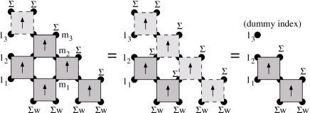
Figure 5: $|\psi_{R}\rangle$ is indeed the right eigenvector of $T$ corresponding to the eigenvalue $\lambda_{0}=1$: for $2M=4$, $T_{m_{1}m_{2}m_{3}}^{l_{1}l_{2}l_{3}}|\psi_{R}\rangle^{m_{1}m_{2}m_{3}}=|\psi_{R}\rangle^{l_{1}l_{2}l_{3}}$.

Let us finally emphasize that for small powers of $T$, $T^{k}$ with $k<2M-1$, this simple decomposition does not hold. But this is not relevant, as we take $k$ to infinity in the TMRG.

To arrive at a prescription for the stochastic TMRG density matrix, we must now consider how actual physical information is extracted from the stochastic transfer matrix. This is done by computing expectation values of local operators, averaged over the whole lattice at final time $2M\cdot\Delta t$ by multiplying $\tau$ in the last time step with the local operator, e.g. for the local particle number operator $n(i)$ one has

$$(\tau_{n})_{l_{1}r_{1}}^{l_{2}r_{2}}:=(\tau)_{l_{1}r_{1}}^{l_{2}r_{2}}\cdot n(l_{2})$$ (15)

where we denote the transfer matrix with its last $\tau$ replaced by $\tau_{n}$ as $T_{n}$ (coloured black in the diagram). Then the expectation value of the particle number operator can be calculated as

$$\langle n_{t=2M\cdot\Delta t}\rangle =\lim_{N\to\infty}\frac{\Tr(T^{N}T_{n})}{\Tr(T^{N+1})}=\lim_{N\to\infty}\frac{\Tr\left(\raisebox{-17.07164pt}{\includegraphics{psirltn.eps}}\right)}{\Tr\left(\raisebox{-14.22636pt}{\includegraphics{psirl.eps}}\right)}$$ (16)

$$=\frac{\Tr(|\psi_{R}\rangle\langle\psi_{L}|T_{n})}{\Tr(|\psi_{R}\rangle\langle\psi_{L}|)}=\frac{\langle\psi_{L}|T_{n}|\psi_{R}\rangle}{\underbrace{\langle\psi_{L}|\psi_{R}\rangle}_{1}}=\left(\,\raisebox{-17.07164pt}{\includegraphics{psiltnr.eps}}\,\right)$$ (17)

where we have omitted local transfer matrices that become trivial by summing and used the pictorial construction of the eigenvectors. The computation of expectation values is thus reduced to the computation of the light cone of lattice sites that can possibly influence the particular site at which the operator is measured.

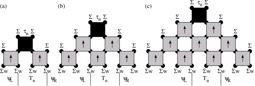
Figure 6: The light cones that are needed to compute the expectation value of the particle number operator for the first few time steps: (a) $2M=2$, (b) $2M=3$, (c) $2M=4$.

Figure 6 shows the light cones for the first few time steps. In this manner one can compute the exact evolution of $\langle n(t)\rangle$, the only inaccuracy stemming from the Trotter-Suzuki decomposition. It is interesting to observe that for determining both eigenvectors and expectation values, a matrix diagonalization can be completely avoided.

For the choice of the density matrix the important observation in figure 6 is now that by parity invariance (7) and adding one dummy index ($i_{2M-1}$),

$$|\psi_{R}\rangle_{2M}^{i_{1}\dots i_{2M-1}}=(\langle\psi_{L}|_{2M-1,\,i_{1}\dots i_{(2M-1)-1}})^{T}=:|\psi_{L}\rangle_{2M-1}^{i_{1}\dots i_{2M-2}}$$ (18)

i.e. the left eigenvector for a given time step is identical to the right eigenvector in the next (half) time step.

3 Density matrix renormalization of the stochastic transfer matrix

We have seen how, in principle, physical information can be extracted from the stochastic transfer matrix, but both memory usage and computation time grow exponentially with the number of time steps. The transfer matrix operates on the space of possible time evolutions of particular sites, which has to be decimated to remain numerically manageable. This is the idea of the TMRG. As the probability of a partial time evolution is determined not only by its past but also by its future continuation, and the infinite future is not yet known, one contends oneself with a “lookahead” of several time steps which is called the “environment”, while the past time evolution — that is being projected onto a smaller Hilbert space — is called the “system”.

Traditionally, one obtains this basis by computing the reduced density matrix for the system, $\rho_{\text{sys}}$, by taking a partial trace over the environment of the outer product of right and left $T$ eigenvectors; the new Hilbert space basis consists of $\rho_{\text{sys}}$’s eigenvectors associated to the largest eigenvalues (highest probabilities). Inspired from traditional TMRG (with periodic b.c. in time direction), one could try $\rho_{\text{sys}}^{\text{asym}}=\Tr_{\text{env}}|\psi_{R}\rangle\langle\psi_{L}|$. But in the case of open b.c., this is just a partial trace of the transfer matrix,

$$\rho_{\text{sys}}^{\text{asym}}=\Tr_{\text{env}}|\psi_{R}\rangle\langle\psi_{L}|=\Tr_{\text{env}}T^{2M-1}=|\psi_{R}\rangle_{\text{sys}}\langle\psi_{L}|_{\text{sys}}$$ (19)

having a spectrum of

$$\text{Spec}(\rho_{\text{sys}}^{\text{asym}})=\{1,0,\dots,0\}.$$ (20)

We demonstrate this for $2M=4$, taking e.g. the first index as the system index and the following two indices as environment indices. Then the trace over the environment $\Tr_{\text{env}}=\sum_{l_{3}r_{3}l_{2}r_{2}}\delta_{l_{3}}^{r_{3}}\delta_{l_{2}}^{r_{2}}$, as illustrated in figure 7, makes all $\tau$’s in the environment trivial: when we contract the dummy index $l_{3}$ with $r_{3}$, the final $\tau$ of $\langle\psi_{L}|$ becomes trivial, so $r_{2}$ now becomes a dummy index. This in turn gives a sum over $l_{2}$, making also the final $\tau$ of $|\psi_{R}\rangle$ trivial, etc. In the end we are left with $|\psi_{R}\rangle$ and $\langle\psi_{L}|$ of an earlier time step, namely the one with only the system indices $l_{1}$, $r_{1}$.

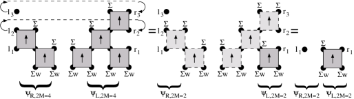
Figure 7: Computing the asymmetrical density matrix $\rho_{\text{sys}}^{\text{asym}}$: the trace makes the environment trivial, $\Tr_{\text{env}}|\psi_{R}\rangle\langle\psi_{L}|=|\psi_{R}\rangle_{\text{sys}}\langle\psi_{L}|_{\text{sys}}$.

Thus this asymmetrical density matrix provides only a single basis vector for the Hilbert space projection, which is obviously not enough. The reason is that the open b.c. “average away” the physical interaction in the environment by making it irrelevant how the system will react in the future. In these boundary conditions resides the essential difference between quantum and stochastic TMRG.

Each renormalization step using $\rho_{\text{sys}}^{\text{asym}}$ projects therefore onto a one-dimensional Hilbert space. No longer-ranged correlation implicit in differently weighted basis vectors is being built up. We therefore expect to observe only the local evolution of the model, which is exactly what we got from numerical simulation using the asymmetrical density matrix.

As an example, we use an exactly solvable reaction-diffusion model: $AA\rightarrow 00$ with rate $2\alpha$ (reaction) and $A0\leftrightarrow 0A$ with rate $D$ (diffusion). For $2\alpha=D$, the exact solution is given by Spouge[16]: for initial partical number $n(t=0)={\textstyle\frac{1}{2}}$ (unbiased $w(0)=w(A)={\textstyle\frac{1}{2}}$, i.e. all lattice sites have an independent probability ${\textstyle\frac{1}{2}}$ of occupancy),

$$\langle n(t)\rangle={\textstyle\frac{1}{2}}\exp(-2Dt)\left[I_{0}(2Dt)+I_{1}(2Dt)\right]\sim\frac{1}{\sqrt{t}}\quad\text{(asympt.)}$$ (21)

This agrees well only with the simulation using the symmetrized density matrix $\rho_{\text{sys}}^{\text{symm}}$ (cf. figure 8). But when we instead use the asymmetrical density matrix $\rho_{\text{sys}}^{\text{asym}}$, we observe a $1/t$ decay. This resembles very closely what we expect from a local interaction: the exact 4-site interaction (i.e. renormalizing as soon as the system has $n$ states) is

$$\langle n(2M+1)\rangle=\langle n(2M)\rangle-[1-\exp(-D\Delta t)]\cdot\langle n(2M)\rangle^{2}$$ (22)

($n(0)={\textstyle\frac{1}{2}}$) which goes asymptotically as $1/t$.

Figure 8: Comparing the simulation of a reaction-diffusion model for symmetrized vs. asymmetrical density matrices. (——) exact solution, (-  -  -  -) exact local (4-site) interaction, (○) simulation, symmetrized density matrix, (◆) simulation, asymmetrical density matrix ($D=0.1$ in inverse time units, and $\Delta t=1$).

The origin of this shortcoming becomes clear in the following consideration: figure 9 shows the left eigenvectors during consecutive time steps. Suppose we want to find a good basis for renormalizing $\langle\psi_{L}|_{2M=5}$, taking its first two indices ($l_{1}$, $l_{2}$) as system and the latter two ($l_{3}$, $l_{4}$) as environment. After somehow tracing over the environment, the new basis vectors will have indices $l_{1}$, $l_{2}$, and they will roughly resemble $\langle\psi_{L}|_{3}$, having a strong correlation between $l_{1}$ and $l_{2}$ because they are connected by an edge of $\tau$.

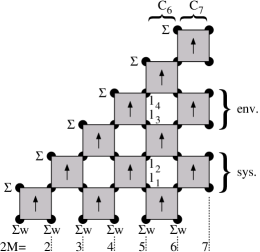
Figure 9: The evolution of the largest left $T$ eigenvector $\langle\psi_{L}|_{2M}$ for the first few Trotter steps.

Now in order to advance one time step from $\langle\psi_{L}|_{5}$ to $\langle\psi_{L}|_{6}$, we see from figure 9 that we need to multiply $\langle\psi_{L}|_{5}$ by the matrix represented by the column $C_{6}$. This reveals the problem: the first two indices of $C_{6}$ are not connected by an edge of $\tau$ and therefore completely independent. Thus the renormalization basis obtained from $\langle\psi_{L}|_{5}$ with a strong correlation between the first pair of indices fits very poorly for renormalizing $C_{6}$. The states in the basis are essentially orthogonal to those that would describe a renormalized $C_{6}$ well. Looking ahead, $C_{7}$ which would bring us to $\langle\psi_{L}|_{7}$ has again a structure similar to $\langle\psi_{L}|_{5}$ and could be renormalized well.

This problem would be remedied by adding to the renormalization basis also basis vectors of a form similar to $\langle\psi_{L}|_{4}$ (tracing over the last index as environment) which shows little correlation between the first two indices. Noting that $\langle\psi_{L}|_{4}=(|\psi_{R}\rangle_{5})^{T}$ (18) we have to mix left and right eigenvectors, $\langle\psi_{L}|_{5}$ and $\langle\psi_{R}|_{5}$, in order to obtain a good basis. Based on the original argument by White[1] about the optimal density matrix in DMRG, Carlon et al[11] have shown that in order to express two different vectors $|\psi_{L}\rangle$, $|\psi_{R}\rangle$ most accurately (in the same basis), one has to use an eigenbasis of $\rho_{\text{sys}}=\Tr_{\text{env}}(|\psi_{R}\rangle\langle\psi_{R}|+|\psi_{L}\rangle\langle\psi_{L}|)$. The symmetrical form of this density matrix arises because they used as a measure of distance between exact and approximated vectors the symmetrical norm $\||\psi_{R}\rangle-\tilde{|\psi_{R}\rangle}\|^{2}+\||\psi_{L}\rangle-\tilde{|\psi_{L}\rangle}\|^{2}$. With this same argument, we now conclude that this symmetrized density matrix is also optimal in the case of explicit eigenvectors.

This explains why a symmetrized density matrix, e.g. $\rho_{\text{sys}}^{\text{symm}}=\Tr_{\text{env}}(|\psi_{R}\rangle\langle\psi_{R}|+|\psi_{L}\rangle\langle\psi_{L}|)$ as used by Kemper et al[15], works so well. Indeed, within the precision of the method, the exact result for the example considered is reproduced when we use this symmetrized reduced density matrix $\rho_{\text{sys}}^{\text{symm}}$.

If we consider for our example the eigenvalue spectrum of the symmetrized density matrix, initially it falls off approximately exponentially, $\lambda_{i}\sim\alpha^{-i}$ for some constant $\alpha$ (cf. figure 10). After many renormalization steps, the spectrum falls off rather according to a power law with large negative exponent, $\lambda_{i}\sim i^{-\beta}$. The symmetrized density matrix therefore indeed fulfills two basic requirements: It should have as many nonzero eigenvalues as possible in order to keep rich nontrivial information about the future evolution in the environment (contrary to (20)), but at the same time they should drop off as quickly as possible so that when we truncate the spectrum at $m$ states that are retained, we lose as little information on the system as possible.

Figure 10: Spectrum of the reduced system density matrix $\rho_{\text{sys}}^{\text{symm}}$ at specific steps $2M$ ($m=64$). (○) $2M=18$ (trunc. $10^{-40}$), (◆) $2M=20$ (trunc. $10^{-29}$), (▽) $2M=60$ (trunc. $10^{-21}$), (□) $2M=280$ (trunc. $10^{-21}$).

Now, in practical applications of the quantum TMRG, system and environment are treated on an equal basis, renormalizing the system with a density matrix traced over the environment and vice versa. In the stochastic TMRG, the explicit construction of $T$ and the eigenvectors opens the possibility to renormalize only the system and keep the environment as a “lookahead” of constant finite length. This simplifies the algorithm, since the $\psi$’s can be renormalized explicitly as shown above, and there is no need to ever solve the eigenvalue problem of the transfer matrix; on the other hand, due to the exponential growth of the matrices with a longer lookahead, this approach is in practice limited (see our numerical example below), and one reverts to the conventional approach of renormalizing both system and environment of the transfer matrix $T$ and then finding its largest eigenvectors anew in each step by using a suitable algorithm for the diagonalisation of large nonsymmetrical matrices.

Our considerations above were all for the case without renormalized environment. Renormalizing it, too, leads to an increasingly longer, but less precise lookahead. As our considerations hold formally for all lengths of lookaheads, the result on the choice of the density matrix should hold also in that case, which is indeed what we observe numerically. To check whether our special choice of a symmetrical density matrix is indeed optimal among symmetrical density matrices, we have also considered numerically several other symmetrical density matrices for comparison, in particular

$$\Tr_{\text{env}}(|\psi_{L}\rangle\langle\psi_{R}|+|\psi_{R}\rangle\langle\psi_{L}|),$$ (23)

$$\Tr_{\text{env}}(|\psi_{L}\rangle+|\psi_{R}\rangle)(\langle\psi_{L}|+\langle\psi_{R}|),$$ (24)

$$\Tr_{\text{env}}(|\psi_{L}\rangle-|\psi_{R}\rangle)(\langle\psi_{L}|-\langle\psi_{R}|),$$ (25)

but the convergence turned out to be worse than for $\rho_{\text{sys}}^{\text{symm}}$. All results shown in the following are therefore for the “canonical” choice of the symmetrical density matrix.

As an application, we tried the branching-fusing process explained in [11]: diffusion $A0\leftrightarrow 0A$ (rate $D$), and several reactions $AA\to 00$ (rate $2\alpha$), $AA\to 0A,A0$ (rate $\gamma$), $0A,A0\to 00$ (rate $\delta$), and $0A,A0\to AA$ (rate $\beta$). The relations between the rates are fixed as $D=2\alpha=\gamma=\delta=1-p\,,\;\;\beta=p$. There is a critical point of the directed percolation universality class at $p_{c}\approx 0.8403578$. First we check the dependence of our TMRG simulation (using the conventional algorithm) for different values of $m$ (number of states kept during projection into a smaller Hilbert space) (cf. figure 11) at the critical point, the most difficult point for the stochastic TMRG.

Figure 11: Branching-fusing model[11] at the critical point $p=0.8403578$ for different number of states kept ($m$) resp. truncation in the spectrum of $\rho_{\text{sys}}$.

We observe that the particle number generally decays exponentially, despite criticality, because we are operating at very short times and due to the rather rough Trotter decomposition. On the lower branch, for a fixed Trotter time $(\Delta t=1)$, our results become more accurate as we increase $m$, effectively truncating the spectrum of $\rho_{\text{sys}}$ at a smaller eigenvalue, until we reach the machine precision (53 mantissa bits). To compute more time steps, one option is to use more accurate floating point numbers (see below).

For comparison, choosing a smaller time step $\Delta t$ (i.e. a finer Trotter decomposition, last two curves in figure 11), while maintaining a large Hilbert space ($m=32$), we get very different results: the particle number decreases much more slowly, which shows that our Trotter decomposition is still far from being sufficiently fine (of course, extrapolations $\Delta t\rightarrow 0$ are feasible). Unfortunately the number of time steps we can simulate decreases, too, which makes such an extrapolation more difficult. This can be explained as follows: the shorter the time step $\Delta t$, the smaller the transition probabilities to different states, and the closer is $\tau$ to the identity matrix. But a transfer matrix composed of such $\tau$’s has eigenvectors with exponentially growing Euclidean norm ($\langle\psi_{R}|\psi_{R}\rangle\sim n^{M}$ and analogously for $|\psi_{L}\rangle$). This is not changed by renormalization because an orthogonal transformation conserves the norm, and we only lose those Hilbert space directions that are very improbable. As the renormalization keeps the number of components of $\langle\psi_{L}|$ and $|\psi_{R}\rangle$ bounded, the values of the components have to grow exponentially to obtain a growing norm. At the same time, $\langle\psi_{L}|\psi_{R}\rangle=1$, so $\langle\psi_{L}|$ and $|\psi_{R}\rangle$ are almost orthogonal. Now the numerical problem is the following: while the components grow exponentially, they have to cancel each other very accurately in order to yield the correct normalization. This works only until the components are of order of magnitude $\sqrt{1/\epsilon}$, where $\epsilon$ is the machine accuracy. Choosing more accurate floating point numbers, by taking twice as many mantissa bits we can simulate very roughly twice as many time steps. This is illustrated in figure 11: if we use the GNU multiprecision library (GMP), truncating at $10^{-21}$ instead of $10^{-15}$, we can simulate approximately 1.5 times as many steps.

Finally we want to compare the numerical stability of the conventional TMRG algorithm, renormalizing both system and environment, with the newly proposed method of explicitly constructing the eigenvectors (saving the iterations of the transfer matrix diagonalisation which take up more than half of the time in the original algorithm). Here we renormalize only the system, keeping a lookahead of finite length as environment. As can be seen in figure 12, the result is much better than the conventional algorithm for an intermediate accuracy of $m=11$ states kept, while it cannot compete with the most accurate (up to machine precision) values for $m=28$. So, as already mentioned above, it is more proof of a concept and a tool for analytical derivations than for practical simulations. Neither more sites lookahead nor larger $m$ improve the result significantly. The computation time for the displayed curves was in the range of a few seconds ($m=11$) up to a few tens of seconds ($m=32$) on a PIII (500 MHz), while memory usage was at most a few MBytes.

Figure 12: Branching-fusing model[11] at the critical point $p=0.8403578$ for different TMRG methods. (——) conventional method, $m=28$; (-  -  -  -) conventional method, $m=11$; (○) explicit eigenvectors, $m=8$ (4 sites lookahead); (◆) explicit eigenvectors, $m=11$ (6 sites lookahead).

4 Conclusions and Outlook

We have shown a new way of looking at stochastic TMRG with open b.c. by explicitly giving the transfer matrix and its left and right eigenvectors corresponding to the physically relevant eigenvalue 1. This allowed us to study the physical effect of various choices for the density matrix of the TMRG. The conclusion was that, unlike the TMRG for quantum transfer matrices, an unsymmetrical density matrix is not just less accurate, but fundamentally unsuitable for the stochastic TMRG. The core problem was that one has open boundary conditions in the future of the time evolution, averaging away the physical interaction, which is not the case in the periodically closed quantum transfer matrix DMRG. The symmetrical density matrix defined by demanding an optimal representation of both left and right eigenvectors in the truncated basis turned out to be the mandated choice. An important observation was that in certain problem classes where small transition probabilities lead to local transfer matrices close to unity, there is an inherent problem with the finite precision of computer arithmetic if one wants to have fine Trotter decompositions and to access comparatively large real times simultaneously.

References

References

- [1] White S R 1992 Phys. Rev. Lett.69 2863 White S R 1993 Phys. Rev.B 48 10345
- [2] Peschel I, Wang X, Kaulke M and Hallberg K (eds.) 1999 Density Matrix Renormalization (Heidelberg: Springer)
- [3] Nishino T 1995 J. Phys. Soc. Japan64 3598
- [4] Bursill R J, Xiang T and Gehring G A 1996 J. Phys.: Condens. Matter8 L583
- [5] Wang X and Xiang T 1997 Phys. Rev.B 56 5061
- [6] Shibata N 1997 J. Phys. Soc. Japan66 2221
- [7] Maisinger K and Schollwöck U 1998 Phys. Rev. Lett.81 445
- [8] Nishino T and Shibata N 1999 J. Phys. Soc. Japan68 1537
- [9] Hieida Y 1998 J. Phys. Soc. Japan67 369
- [10] Kaulke M and Peschel I 1998 Eur. J. Phys.B 5 727
- [11] Carlon E, Henkel M and Schollwöck U 1999 Eur. J. Phys.B 12 99
- [12] Carlon E, Henkel M and Schollwöck U 2001 Phys. Rev.E 63 036101
- [13] Carlon E, Drzewinski A and van Leeuwen J M J 2000 Preprint cond-mat/0010177
- [14] Henkel M and Schollwöck U 2001 J. Phys. A: Math. Gen.34 3333
- [15] Kemper A, Schadschneider A and Zittartz J 2001 J. Phys. A: Math. Gen.34 L279
- [16] Spouge J L 1988 Phys. Rev. Lett.60 871