Tube Model for the Elasticity of Entangled Nematic Rubbers

Abstract

Dense rubbery networks are highly entangled polymer systems, with significant topological restrictions for the mobility of neighbouring chains and crosslinks preventing the reptation constraint release. In a mean field approach, entanglements are treated within the famous reptation approach, since they effectively confine each individual chain in a tube-like geometry. We apply the classical ideas of reptation dynamics to calculate the effective rubber-elastic free energy of anisotropic networks, nematic liquid crystal elastomers, and present the first theory of entanglements for such a material.

PACS numbers:
61.41.+e  Polymers, elastomers, and plastics
61.20.Vx  Polymer liquid crystals
62.20.Dc  Elasticity, elastic constants

1 Introduction

Rubbery polymer networks are complex randomly disordered amorphous systems. The simplest theoretical models consider them as being made of “phantom chains”, where each chain is thought to be a three-dimensional random walk in space. To form a network, the chains are crosslinked to each other at their end points, but do not interact otherwise, in particular they are able to fluctuate freely between crosslinks. This has an unphysical consequence that the strands can pass through each other. If one tries to avoid this assumption, the theory is confronted with the intractable complexity of entanglements and their topological constraints. The mean field treatment of entangled polymer melts and semi-dilute solutions is the classical reptation theory [1, 2] going back to the early seventies, which has been a spectacular success in describing a large variety of different physical effects. However, the parallel description of crosslinked rubbery networks has been much less successful. First of all, there is a significant difference in entanglement topology: in a melt the confining chain has to be long enough to form a topological knot around a chosen polymer; even then the constraint is only dynamical and can be released by a reptation diffusion along the chain path. In a crosslinked network, any loop around a chosen strand becomes an entanglement, which could be mobile but cannot be released altogether. A number of other complexities arise from the coupling between imposed deformations and chain anisotropy, the stress-optical effects [3, 4, 5] and nematic interactions between chain segments [6, 7].

In addition, the polymer network can be spontaneously anisotropic, forming a liquid crystalline elastomer (LCE). This area has attracted a significant experimental and theoretical interest in recent years. In nematic LCE, the strands preferably orient themselves along one direction, forming a nematic liquid crystal order. The response to an external deformation is now of a much richer nature, with antisymmetric stress and internal torques depending on the relative angle of the director to the axis of deformation [8]. Liquid crystalline elastomers combine remarkable properties of both its components, liquid crystals and rubbers, but also show physical properties that place them in a separate category from any other material. Several new physical phenomena have been discovered in LCE: (a) spontaneous, reversible shape changes of up to 400% on temperature change; (b) “soft elasticity” – mechanical deformation, involving modifications of internal nematic microstructure, without (or with very low) stress; (c) mechanical and electric instabilities involving director reorientation, in special cases discontinuous jumps; (d) solid phase nematohydrodynamics and unusual rheology, leading to anomalous dissipation and acoustic effects. Recent reviews [9, 10] describe the current state of affairs in this field. Our challenge in this paper is to bring the microscopic theoretical description of nematic rubbers on the same level as in the classical isotropic rubbers, in particular, to account for chain entanglements.

An early model of elastic response of entangled rubbers was developed by Edwards [11]: in tradition with the melt theory, it assumed that the presence of neighbouring strands in a dense network effectively confines a particular polymer strand to a tube, whose axis defines the primitive path. Within this tube, the polymer is free to explore all possible configurations, performing random excursions, parallel and perpendicular to the axis of the tube. One can show that on deformation of the sample the length of the primitive path increases. Since the arc length of the polymer is constant, the amount of chain available for perpendicular excursions is reduced, leading to a reduction in entropy and an increase in rubber-elastic free energy. A number of further attempts have been made to derive a self-consistent theory of entangled rubber elasticity. Of this list, the most significant are the scaling “localisation model” of Gaylord and Douglas [12], the “slip-link model” of Ball, Doi, Edwards and Warner (BDEW) [13], accounting for entanglements as local mobile confinement sites linking two interwound strands, and the “hoop model” by Higgs and Ball (HB) [14], who assumed that entanglements localise certain chain segments. In an article developing the reptation theory of rubber elasticity for classical isotropic networks [15], we give a more detailed overview of these and other theories.

In our current work, we extend the tube model to treat the elasticity of anisotropic networks of liquid crystalline polymers. To our knowledge, this is the first time that a reptation model has been applied to treat the effects both of the entanglements and of the anisotropic nature of the nematic network. The tube model provides a more accurate microscopic description in the sense that it keeps track of the allocation of chain segments and their excursions between the points of entanglement. The next Section briefly reviews the ideal phantom-network approach to the elasticity of nematic rubber and introduces the tube model and its properties, giving the full expression for nematic rubber-elastic free energy. Section 3 contains the discussion of the model and its results, including the linear-response limit. We conclude by comparing the results of the present theory with those of the ideal phantom network and analyse which physical properties of LCE seem to be most sensitive to the effect of chain entanglements.

2 Nematic elastomer network

Before developing our model for macroscopic elasticity of densely entangled rubber, we briefly review the well-known results of the phantom chain network theory, which provides the basics to most other theoretical models.

Phantom chain approximation

Assuming that a single polymer performs a free random walk in three dimensions, one finds that the end-to-end distance ${\bm{R}}_{0}$ obeys a Gaussian distribution in the long chain limit. This result goes back far in history: one can review its derivation and consequences in the classical text on this subject [2]. The distribution of $\bm{R}_{0}$ is given by

$$P_{0}({\bm{R}}_{0})=\left(\frac{3}{2\pi Nb^{2}}\right)^{3/2}\exp\left(-\frac{3}{2Nb^{2}}{\bm{R}}_{0}^{2}\right),$$ (1)

where $b$ is the monomer step length and $N$ the number of steps of one chain trajectory.

In a nematic polymer, irrespective of the particular mesogenic mechanism, the monomer steps acquire a preferred orientation along the director $\bm{n}_{0}$. Accordingly, the end-to-end distance distribution function of a strand becomes anisotropic as well:

$$P(\bm{R_{0}}) = \left(\frac{3}{2\pi Nb}\right)^{3/2}(\det\underline{\underline{\ell}}_{0})^{-1/2}$$

$$\times\exp\left(-\frac{3}{2L}\bm{R}_{0}^{\mathsf{T}}\cdot\underline{\underline{\ell}}_{0}^{-1}\cdot\bm{R}_{0}\right),$$

where $Nb=L$ is the contour length of the chain, and the matrix $\underline{\underline{\ell}}_{0}$takes account of the anisotropy:

$$(\underline{\underline{\ell}}_{0})_{ij}=l_{0}^{\perp}\delta_{ij}+(l_{0}^{\parallel}-l_{0}^{\perp})n_{0i}n_{0j}.$$

This matrix of anisotropic chain steps is directly measurable from the average chain shape, given by $\langle R_{i}R_{j}\rangle=\frac{1}{3}(\underline{\underline{\ell}}_{0})_{ij}L$. The principal values of this effective step-length matrix, $l_{0}^{\perp}$ and $l_{0}^{\parallel}$, reflect the spontaneous nematic order in the material. In the isotropic phase, e.g., above the nematic transition temperature $T_{\rm ni}$, $l_{0}^{\parallel}=l_{0}^{\perp}=b$ and one trivially recovers the isotropic Gaussian distribution (1). The difference $l_{0}^{\parallel}-l_{0}^{\perp}$ is proportional to the nematic order parameter $Q$. However, the explicit form of this dependence is different in different models of nematic polymers. In a most simple case of freely jointed chain of rods of length $b$ one obtains $l_{0}^{\parallel}=b(1+2Q),\ l_{0}^{\perp}=b(1-Q)$, while in the hairpin regime of semiflexible main-chain nematic polymer the anisotropy could become very large: $l_{0}^{\parallel}\propto\exp[3/(1-Q)]$, cf. [16]. The power of the ideal theory of nematic rubber elasticity [8] is in that it is independent of such model considerations and only uses a single model parameter – the ratio $r=l_{0}^{\parallel}/l_{0}^{\perp}$, or equivalently, $r=\langle R_{\parallel}^{2}\rangle/\langle R_{\perp}^{2}\rangle$ for the principal values of the gyration radius. We shall see below that this attractive feature is reproduced in the theory of entangled nematic networks.

The entropic free energy of such an anisotropic random walk is given by the logarithm of the number of conformations with the fixed $\bm{R}_{0}$ and has the form

$$\beta F=-\ln P({\bm{R}}_{0})=\frac{3}{2L}\bm{R}_{0}^{\mathsf{T}}\cdot\underline{\underline{\ell}}_{0}^{-1}\cdot\bm{R}_{0}+\mathrm{const},$$

where $\beta=1/k_{B}T$ is the inverse Boltzmann temperature. At formation of the network, i.e. at crosslinking, the polymer melt is assumed to obey the anisotropic Gaussian distribution (2), which is then permanently frozen in the network topology. In the phantom network approximation, the lateral restrictions on the chain thermal motion are neglected and different network strands interact only at the crosslinking points.

One then assumes that the junction points deform affinely with respect to their initial positions $\bm{R}_{0}$ by the macroscopic deformation $\underline{\underline{{\bm{\lambda}}}}$, hence we can write $\bm{R}=\underline{\underline{{\bm{\lambda}}}}\bm{R}_{0}$. Therefore, the deformation $\underline{\underline{{\bm{\lambda}}}}$ alters the free energy of each strand. The change of free energy per chain of the whole network can be calculated by the usual quenched averaging:

$$\beta F=-\langle\ln P(\underline{\underline{{\bm{\lambda}}}}\bm{R}_{0})\rangle_{P(\bm{R}_{0})}=\frac{1}{2}\mathrm{Tr}(\underline{\underline{\ell}}_{0}\cdot\underline{\underline{{\bm{\lambda}}}}^{\mathsf{T}}\cdot\underline{\underline{\ell}}_{\theta}^{-1}\cdot\underline{\underline{{\bm{\lambda}}}}),$$ (3)

where we have dropped an irrelevant constant and found a new expression for the chain step-length matrix after deformation:

$$(\underline{\underline{\ell}}_{\theta})_{ij}=l^{\perp}\delta_{ij}+(l^{\parallel}-l^{\perp})n_{i}n_{j},$$

with the rotated director, $(\bm{n}\cdot\bm{n}_{0})=\cos\theta$, and possibly changed principal values $l^{\parallel}$ and $l^{\perp}$. The overall elastic free energy density, in the first approximation, is simply (3) multiplied by the number of elastically active network strands in the system $n_{\rm ch}$ per unit volume, which is proportional to the crosslinking density:

$$F_{\rm el}=\frac{1}{2}\mu\ \mathrm{Tr}(\underline{\underline{\ell}}_{0}\cdot\underline{\underline{{\bm{\lambda}}}}^{\mathsf{T}}\cdot\underline{\underline{\ell}}_{\theta}^{-1}\cdot\underline{\underline{{\bm{\lambda}}}}),$$ (4)

with the rubber modulus $\mu=n_{\rm ch}k_{B}T$, cf. [8] for detail.

The phantom-network model of rubber elasticity is a popular first approximation. There are several reasons for its overall success in spite of obvious oversimplifications. The crosslinking points connect the ends of different strands together and thus reduce local fluctuations – and, therefore, alter the single chain statistics. However, in spite of an apparent complexity of this problem, it has been shown [17] that this effect merely introduces a trivial multiplicative factor of the form $1-2/\phi$, where $\phi$ is the junction point functionality. Secondly, one can assume that the deformation preserves the volume, since the bulk (compression) modulus is by a factor of at least $10^{4}$ greater than the shear modulus, which is proportional to $\mu$; this implies the constraint $\det\underline{\underline{{\bm{\lambda}}}}=1$. Thirdly, the quenched average in equation (3) does not average over chains of different arc lengths, but the fact that the result is independent of arc length, generalises the result to apply for chains of arbitrary length, or even for a polydisperse ensemble of chains. In the particular case of nematic LCE, this simple model provides a rich crop of theoretical predictions described in greater detail in quoted review articles.

The tube model

Following the original ideas of Edwards [11], we assume that one particular network strand is limited in its lateral fluctuations by the presence of neighbouring chains. Therefore each segment of a given strand only explores configurations in a limited volume, which is much smaller than in the random coil state. Hence, the whole strand fluctuates around a mean path, which we call the primitive path. Effectively, the chain is confined to exercise its thermal motion only within a tube around the primitive path due to the presence of neighbouring chains. This primitive path itself can be considered as a random walk with an associated typical step length, which is much bigger than the monomer step length [18]. The step length of the primitive path divides the tube into tube segments, as sketched in Fig. 1, and therefore determines the number of tube segments $M$ along one polymer strand.

Note that all chains are in constant motion, altering the local constraints they impose on each other. Hence, the tube is a gross simplification of real situation. However, one expects this to be an even better approximation in rubber than in a corresponding melt (where the success of reptation theory is undeniable), because the restriction on chain reptation diffusion in a crosslinked network eliminates the possibility of constraint release.

To handle the tube constraint mathematically, we assume that the chain segments are subjected to a quadratic potential, restricting their motion transversely to the primitive path. Along one polymer strand consisting of $N$ monomers of effective step length $b$, there are $M$ tube segments, each containing $s_{m},\ m=1,\dots,M$ monomer steps. We infer the obvious condition

$$\sum_{m=1}^{M}s_{m}=N.$$ (5)

In effect, one has two random walks: the topologically fixed primitive path and the polymer chain restricted to move around it – both having the same end-to-end vector $\bm{R}_{0}$, between the connected crosslinking points.

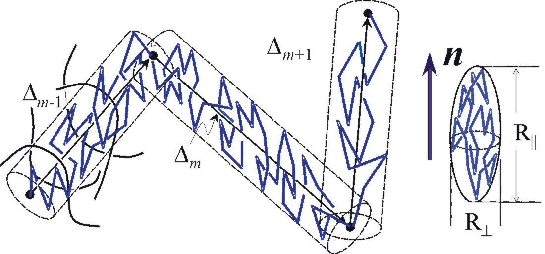
Figure 1: A nematic polymer strand is surrounded by neighbouring chains, which effectively confine the strand to a tube. The tube segment $m$ contains $s_{m}$ monomer steps, where the index $m$ runs from 1 to $M$. Since the direction of chain steps is, on average, uniaxial (as illustrated by the drawing of an ellipsoidal shape of a free chain gyration on the right), the number of steps in each tube segment depends on the orientation of $\bm{\Delta}_{m}$ with respect to the nematic director $\bm{n}$.

Each tube segment $m$ can be described by the span vector $\bm{\Delta}_{m}$, joining the equilibrium positions of the strand monomers at the two ends of each tube segments. The number of tube segments $M$ (or, equivalently, the number of chain entanglements, $M-1$) is a free parameter of the theory, ultimately determined by the length of each polymer strand and the average “entanglement density”.

Since the primitive path is a topologically frozen characteristic of each network strand, we shall assume that all primitive path spans $\bm{\Delta}_{m}$ deform affinely with the macroscopic strain: $\bm{\Delta}_{m}^{\prime}=\underline{\underline{{\bm{\lambda}}}}\bm{\Delta}_{m}$. This is the central point in the model: the rubber elastic response will arise due to the change in the number of polymer configurations in a distorted primitive path. To evaluate the number of conformations, we look separately at chain excursions parallel and perpendicular to the tube axis, within each span $\bm{\Delta}_{m}$. Effectively, this amounts to introducing a new coordinate system for each tube segment, with one preferred axis along $\bm{\Delta}_{m}$. The constraints exerted by the other chains only constrain the considered polymer in its lateral motion. Hence, we recover the behaviour of a one-dimensional random walk in the direction of $\bm{\Delta}_{m}$, giving rise to Gaussian statistics in the long chain limit. Note that only one third of the steps $s_{m}$ in this tube is involved in the longitudinal excursions. We therefore obtain for the number of longitudinal excursions in a tube segment $m$, cf. Fig. 1,

$$W_{m}^{\rm(L)}\propto\frac{1}{\sqrt{s_{m}/3}}\exp\left(-\frac{1}{2b(s_{m}/3)}\bm{\Delta}_{m}^{\mathsf{T}}\cdot\underline{\underline{\ell}}_{0}^{-1}\cdot\bm{\Delta}_{m}\right).$$ (6)

The spontaneous anisotropy of nematic polymer chain is reflected in (6) by accounting for the difference in number of chain conformations in a given tube segment, depending on its orientation with respect to the local nematic director (the principal axis of step-length matrix $\underline{\underline{\ell}}_{0}$).

To determine the number of transverse excursions, we introduce the Green’s function for the steps made by the chain in the plane perpendicular to the local tube axis $\bm{\Delta}_{m}$. In effect, we consider a two-dimensional random walk, with a total number of steps $(2s_{m}/3)$, in a centrosymmetric quadratic potential. For each of these two perpendicular coordinates, the Green’s function satisfies the following modified diffusion equation (see e.g. [2], and its extension for the uniaxial nematic case in [17]). The argument that follows, about transverse chain movements in a confining potential, has a very simple conclusion – that the conformational effects are irrelevant for calculation of rubber elasticity and only important factor is the number of chain steps attributed to this degree of freedom. Equally, the anisotropic (nematic) nature of chain random walk does not contribute to the entropy of strongly confined transverse excursion. Although the full anisotropic treatment is possible, here we shall use a much shorter and transparent version of the isotropic chain confined in the tube; its Green’s function satisfies the differential equation for each of the two coordinates:

$$\left(\frac{\partial}{\partial s}-\frac{1}{2}b^{2}\frac{\partial^{2}}{\partial x_{f}^{2}}+\frac{1}{2}q_{0}^{2}x_{f}^{2}\right)G(x_{i},x_{f};s)=\delta(x_{f}-x_{i})\delta(s),$$ (7)

where the $x_{i}$ and $x_{f}$ are the initial and final coordinates of the random walk with respect to the tube axis and $q_{0}$ determines the strength of the confining potential. The equation (7) is very common in the physics of polymers and its exact solution is known. However, we only need to consider a particular limit $q_{0}bs_{m}\gg 1$ of this solution, which is the case of dense entanglements (resulting in a strong confining potential) and/or of a large number $s_{m}$ of monomers confined in the tube segment. Outside this limit, that is, when the tube diameter is the same order as the arc length of the confined chain, the whole concept of chain entanglements becomes irrelevant. In the strongly confined limit the solution has a particularly simple form [11]:

$$G(x_{i},x_{f};s)\propto\exp\left(-\frac{q_{0}}{2b}(x_{i}^{2}+x_{f}^{2})-\frac{1}{6}q_{0}bs_{m}\right).$$ (8)

Remembering that there are two coordinates describing the transverse excursions, we obtain for the two-dimensional Green’s function of the tube segment $m$:

$$G_{m}(\bm{r}_{i},\bm{r}_{f};s)\propto\exp\left(-\frac{1}{3}q_{0}bs_{m}\right)\exp\left(-\frac{q_{0}}{2b}(\bm{r}_{i}^{2}+\bm{r}_{f}^{2})\right),$$ (9)

where $\bm{r}_{i}$ and $\bm{r}_{f}$ are the initial and final transverse two-dimensional coordinates.

The total number of transverse excursions is proportional to the integrated Green’s function:

$$W_{m}^{\rm(T)}\propto\int d\bm{r}_{i}\int d\bm{r}_{f}G_{m}(\bm{r}_{i},\bm{r}_{f};s).$$

Since the Green’s function (9) does not couple the initial or final coordinates to the number of segments $s_{m}$, this integration will only produce a constant normalisation factor which can be discarded. Exactly the same conclusion is reached if the modified diffusion equation for anisotropic chain is considered.

Gathering the expressions for statistical weights of parallel and perpendicular excursions (and returning to the fully anisotropic description), one obtains the total number of configurations of a polymer segment consisting of $s_{m}$ monomers in a tube segment of span $\bm{\Delta}_{m}$:

$$W_{m} = W_{m}^{\rm(L)}W_{m}^{\rm(T)}$$

$$\propto \frac{1}{\sqrt{s_{m}}}\exp\left(-\frac{1}{3}q_{0}bs_{m}-\frac{1}{2b(s_{m}/3)}\bm{\Delta}_{m}^{\mathsf{T}}\cdot\underline{\underline{\ell}}_{0}^{-1}\cdot\bm{\Delta}_{m}\right).$$

Therefore, we find for the full number of configurations of the whole strand

$$W=\int\limits_{0}^{N}ds_{1}\cdots\int\limits_{0}^{N}ds_{M}\left(\prod_{m=1}^{M}W_{m}\right)\delta\left(\sum_{m=1}^{M}s_{m}-N\right),$$ (11)

where we have implemented the polymer contour length constraint (5). The statistical summation in (11) takes into account the reptation motion of the polymer between its two crosslinked ends, by which the number of segments, $s_{m}$, constrained within each tube segment can be changed and, thus, equilibrates for a given conformation of primitive path.

Rewriting the delta-function as $\delta(x)=\frac{1}{2\pi}\int dk\ e^{{\rm i}kx}$, we proceed by finding the saddle points $s_{m}^{*}$ which make the exponent of statistical sum (11) stationary. It can be verified that the normalisation factors $1/\sqrt{s_{m}}$ contribute only as a small correction to the saddle points

$$s_{m}^{*}\approx\left(\frac{3\ \bm{\Delta}_{m}^{\mathsf{T}}\cdot\underline{\underline{\ell}}_{0}^{-1}\cdot\bm{\Delta}_{m}}{2b(\frac{1}{3}q_{0}b+{\rm i}k)}\right)^{1/2}.$$ (12)

The integral in (11) is consequently approximated by the steepest descent method. We repeat the same procedure for the integration of the single auxiliary variable $k$, responsible for the conservation of the polymer arc length. The saddle point value $k^{*}$, inserted into (12), gives

$$\overline{s}_{m}=\frac{N|\underline{\underline{\ell}}_{0}^{-1/2}\bm{\Delta}_{m}|}{\sum_{i=m}^{M}|\underline{\underline{\ell}}_{0}^{-1/2}\bm{\Delta}_{m}|},$$

which is the equilibrium number of steps the nematic polymer makes in a tube segment characterised by the axis vector $\bm{\Delta}_{m}$. By completing the saddle-point integration, we finally obtain the total number of configurations of one strand, confined within a tube whose primitive path is described by the set of vectors $\{\bm{\Delta}_{m}\}$. The statistical weight $W$ associated with this state is proportional to the probability distribution:

$$W(\bm{\Delta}_{1},\dots,\bm{\Delta}_{M})\propto P(\{\bm{\Delta}_{m}\})$$

$$\propto \frac{\exp\left(-\frac{3}{2bN}\left(\sum_{m=1}^{M}|\underline{\underline{\ell}}_{0}^{-1/2}\bm{\Delta}_{m}|\right)^{2}-\frac{1}{3}q_{0}bN\right)}{\left(\sum_{i=m}^{M}|\underline{\underline{\ell}}_{0}^{-1/2}\bm{\Delta}_{m}|\right)^{M-1}}.$$

The scalar $|\underline{\underline{\ell}}_{0}^{-1/2}\bm{\Delta}_{m}|$ reflects the length of the $m$-th step of the primitive path, modified by its projection on the uniaxial matrix of chain step-lengths. This expression is a result parallel to the ideal Gaussian $P(\bm{R}_{0})$ in equation (2) for a unentangled chain. Note that the chain end-to-end distance $\bm{R}_{0}$ is also the end-to-end distance of the primitive path random walk: $\sum_{m=1}^{M}\bm{\Delta}_{m}=\bm{R}_{0}$.

Free energy of deformations

From the equation (2) we obtain the formal expression for free energy of a chain confined to a tube with the primitive path conformation $\{\bm{\Delta}_{m}\}$, $\beta F=-\ln W$, or

$$\beta F = \frac{3}{2bN}\left(\sum_{m=1}^{M}|\underline{\underline{\ell}}_{0}^{-1/2}\bm{\Delta}_{m}|\right)^{2}$$

$$+(M-1)\ln\left(\sum_{m=1}^{M}|\underline{\underline{\ell}}_{0}^{-1/2}\bm{\Delta}_{m}|\right),$$

where we have dropped irrelevant constants arising from normalisation. We now perform a procedure which is analogous to the one used to obtain equation (3). In the polymer melt before crosslinking, we assume that the ensemble of chains obeys the distribution in (2) giving the free energy per strand (2). The process of crosslinking not only quenches the end points of each of the crosslinked strands, but also quenches the nodes of the primitive path ${\bm{\Delta}}_{m}$, since the crosslinked chains cannot disentangle due to the fixed topology of the network. In our mean field approach, the tube segments described by ${\bm{\Delta}}_{m}$ are conserved. For evaluating the quenched average, note that the statistical weight (2) treats all tube segments $m$ in an equivalent way. This allows one to perform the summation over the index $m$, separating the diagonal and the off-diagonal terms:

$$\beta F = \frac{3}{2bN}\left(M\langle\bm{\Delta}_{m}^{\mathsf{T}}\cdot\underline{\underline{\ell}}_{0}^{-1}\cdot\bm{\Delta}_{m}\rangle\right.$$

$$\ \ \ \ \left.+M(M-1)\langle|\underline{\underline{\ell}}_{0}^{-1/2}\bm{\Delta}_{m}||\underline{\underline{\ell}}_{0}^{-1/2}\bm{\Delta}_{n}|\rangle\right)$$

$$+(M-1)\left\langle\ln\left(\sum_{m=1}^{M}|\underline{\underline{\ell}}_{0}^{-1/2}\bm{\Delta}_{m}|\right)\right\rangle,$$

for arbitrary values of $m$ and $n\neq m$; the brackets $\langle\cdots\rangle$ refer to the average with the probability $P(\{\bm{\Delta}_{m}\})$ given in (2).

Any mechanical deformation expressed by the general strain tensor $\underline{\underline{{\bm{\lambda}}}}$ will affinely transform $\bm{\Delta}_{m}$ into $\bm{\Delta}_{m}^{{}^{\prime}}=\underline{\underline{{\bm{\lambda}}}}\bm{\Delta}_{m}$. It could also affect the nematic order: the director $\bm{n}$ could adopt a different orientation under deformation and the degree of average chain anisotropy $r$ may change as well. In other words, the matrix $\underline{\underline{\ell}}_{0}$, which characterises the anisotropy of the steps, transforms into a new matrix $\underline{\underline{\ell}}_{\theta}$ with different eigenvalues $l^{\parallel}$ and $l^{\perp}$ in a reference frame rotated by the angle $\theta$. Hence $|\underline{\underline{\ell}}_{0}^{-1/2}\bm{\Delta}_{m}|$ transforms into $|\underline{\underline{\ell}}_{\theta}^{-1/2}\underline{\underline{{\bm{\lambda}}}}\bm{\Delta}_{m}|$ on deformation, but the distribution $P(\{\bm{\Delta}_{m}\})$ remains unchanged. Bearing this in mind, we can evaluate the averages (2), leading to the free energy per crosslinked chain. The Appendix gives a more detailed account of how one evaluates the averages. The resulting elastic energy density takes the form

$$F_{\rm el} = \frac{2}{3}\mu\ \frac{2M+1}{3M+1}\,\mathrm{Tr}(\underline{\underline{\ell}}_{0}\cdot\underline{\underline{{\bm{\lambda}}}}^{\mathsf{T}}\cdot\underline{\underline{\ell}}_{\theta}^{-1}\cdot\underline{\underline{{\bm{\lambda}}}})$$

$$+ \frac{3}{2}\mu(M-1)\frac{2M+1}{3M+1}\left(\overline{|\underline{\underline{\ell}}_{\theta}^{-1/2}\cdot\underline{\underline{{\bm{\lambda}}}}\cdot\underline{\underline{\ell}}_{0}^{1/2}|}\right)^{2}$$

$$+ \mu(M-1)\overline{\ln|\underline{\underline{\ell}}_{\theta}^{-1/2}\cdot\underline{\underline{{\bm{\lambda}}}}\cdot\underline{\underline{\ell}}_{0}^{1/2}|},$$

where we use the notations:

$$\overline{|\underline{\underline{\ell}}_{\theta}^{-1/2}\cdot\underline{\underline{{\bm{\lambda}}}}\cdot\underline{\underline{\ell}}_{0}^{1/2}|} = \frac{1}{4\pi}\!\int\limits_{|{\bf e}|=1}\!\!d\Omega|\underline{\underline{\ell}}_{\theta}^{-1/2}\cdot\underline{\underline{{\bm{\lambda}}}}\cdot\underline{\underline{\ell}}_{0}^{1/2}\ {\bf e}|\hskip 28.45274pt$$ (17)

$$\overline{\ln|\underline{\underline{\ell}}_{\theta}^{-1/2}\cdot\underline{\underline{{\bm{\lambda}}}}\cdot\underline{\underline{\ell}}_{0}^{1/2}|} = \frac{1}{4\pi}\!\!\int\limits_{|{\bf e}|=1}\!\!d\Omega\ln|\underline{\underline{\ell}}_{\theta}^{-1/2}\cdot\underline{\underline{{\bm{\lambda}}}}\cdot\underline{\underline{\ell}}_{0}^{1/2}\ {\bf e}|$$ (18)

(the overline notation $\overline{\cdots}$ refers to the angular averaging over the orientations of an arbitrary unit vector e used to contract a corresponding matrix into a vector, before calculating its absolute value).

Expressions (17) and (18) can be evaluated in various particular cases of deformation $\underline{\underline{{\bm{\lambda}}}}$ and director orientation. The Appendix gives a result for uniaxial deformation along the director, where $\underline{\underline{{\bm{\lambda}}}}$ takes a diagonal form with $\lambda^{\parallel}=\lambda$ and $\lambda^{\perp}=1/\sqrt{\lambda}$. Explicit formulae for (17) and (18) need to be inserted into (2) to give the full elastic energy.

3 Discussion

From the expression (2), we can recover the elastic free energy of an ideal phantom-chain nematic network by taking the case $M=1$. This limit means physically that the polymer strand is placed in one single tube, tightly confined to the axis. Mathematically, a random walk in three dimensions with $N$ steps is equivalent to a random walk in one dimension along a given direction with $N/3$ steps. This fact is the underlying reason why we recover the phantom chain network result by taking $M=1$ in our model.

On the other hand, as the number of tube segments $M$ becomes large, one obtains a rubber-elastic elastic energy of the form

$$F_{\rm el}=\mu M\left((\langle|\underline{\underline{\ell}}_{\theta}^{-1/2}\cdot\underline{\underline{{\bm{\lambda}}}}\cdot\underline{\underline{\ell}}_{0}^{1/2}|\rangle)^{2}+\langle\ln|\underline{\underline{\ell}}_{\theta}^{-1/2}\cdot\underline{\underline{{\bm{\lambda}}}}\cdot\underline{\underline{\ell}}_{0}^{1/2}|\rangle\right).$$ (19)

There are two ways to have a physical situation corresponding to this limit of $M\gg 1$: either the polymer melt is very dense, causing a high entanglement density, or the polymer chain is very long between its crosslinked ends. In the latter case, the polymer strand experiences many confining entanglements along its path.

Recall that the $F_{\rm el}$ is the elastic energy density, which relates to the free energy per chain $F$ as: $F_{\rm el}=n_{\rm ch}F$, where $n_{\rm ch}$ is the density of crosslinked strands. We can assume that in a polymer melt, the chain density is inversely proportional to the volume of an average chain, hence inversely proportional to the contour length of this chain: $n_{\mathrm{ch}}\propto 1/L$. In case of the phantom chain network the rubber modulus $\mu=n_{\rm ch}k_{B}T$ [equation (3)]. One concludes in this case that the elastic energy $F_{\mathrm{el}}$ scales with $1/L$, and therefore $F_{\mathrm{el}}\rightarrow 0$ as the chains become infinitely long! This unphysical behaviour reflects the fact that the phantom chain model assumes the entanglement interactions of the chains irrelevant. Clearly, this assumptions breaks down in the long chain limit, where one expects the entanglements to play a crucial role.

This unphysical behaviour is overcome by our expression (19). As the strands become longer, they will experience more entanglements, generating more confining tube segments. We could reasonably assume that the number of entanglements and therefore the number of tube segments scales linearly with the strand length $L$: $M\propto L$. Considering expression (19), one can note that the corresponding rubber modulus does not vanish in the limit $L\rightarrow\infty$, but remains a constant corresponding to the “rubber plateau” in a densely entangled melt.

Considering the particular case of uniaxial strain along the constant nematic director $\bm{n}$, one can examine one of the key physical effects found in nematic elastomers – the spontaneous mechanical deformations as the degree of anisotropy is changed, for instance, by changing the temperature (and thus the nematic order parameter $Q(T)$ and the effective chain anisotropy $r$). Within the ideal phantom-chain model (4), applying a uniaxial deformation along the director $\bm{n}$ with $\lambda^{\parallel}=\lambda$ and $\lambda^{\perp}=1/\sqrt{\lambda}$, one obtains

$$F_{\rm el}=\frac{1}{2}\mu\left(\frac{l_{0}^{\parallel}}{l^{\parallel}}\lambda^{2}+2\frac{l_{0}^{\perp}}{l^{\perp}}\frac{1}{\lambda}\right),$$

where $l_{0}^{\parallel}$ and $l_{0}^{\perp}$ are the principal values of $\underline{\underline{\ell}}_{0}$, and similarly $l^{\parallel}$ and $l^{\perp}$ the ones of $\underline{\underline{\ell}}_{\theta}$, the anisotropy of a state after the deformation (of course, in this case no director rotation occurs). The free energy is minimised by the strain

$$\lambda_{\mathrm{m}}=(l^{\parallel}l_{0}^{\perp}/l_{0}^{\parallel}l^{\perp})^{1/3},$$

which describes a spontaneous uniaxial deformation of a nematic rubber, first discovered theoretically in [17] and mentioned in the literature ever since. For instance, if the initial state $\underline{\underline{\ell}}_{0}$is isotropic (at $T>T_{\rm ni}$), then $\lambda_{\mathrm{m}}=(l^{\parallel}/l^{\perp})^{1/3}$, a function of nematic order parameter $Q(T)$ and could reach a remarkable value of 400% uniaxial extension in a highly anisotropic main-chain nematic rubber [19].

This result is not altered by the complicated additional terms in (2): remarkably, exactly the same deformation $\lambda_{\mathrm{m}}$ minimises all three corresponding expressions derived from (2), which are given in the Appendix.

If we now assume that both the chain anisotropy and the director $\bm{n}$ are kept fixed under the deformation, $\underline{\underline{\ell}}_{\theta}=\underline{\underline{\ell}}_{0}$, and that the strain tensor $\underline{\underline{{\bm{\lambda}}}}$ is diagonal in the reference frame of the anisotropy matrix, then we observe that the matrices in (2)–(18) are all diagonal. Hence the anisotropic terms cancel each other out, and we are left with the same elastic energy as in the isotropic case [15]. Hence, even if the material is anisotropic, its linear elastic modulus does not depend on the orientation under the above assumptions of unchanged degree of anisotropy $r=l^{\parallel}/l^{\perp}$: the Young’s moduli $E^{\parallel}=E^{\perp}=E$. However, the modulus for simple shear is partially affected by the anisotropy of the nematic rubber. Consider $\lambda_{ij}=\delta_{ij}+\varepsilon u_{i}v_{j}$, with ${\bm{u}}$ and ${\bm{v}}$, the two orthogonal unit vectors defining the simple shear. If the deformation does not mix the parallel and perpendicular directions, i.e., if ${\bm{u}}$ and ${\bm{v}}$ are both perpendicular to ${\bm{n}}$, then the shear modulus is the same as in the isotropic case,

$$G=\frac{1}{3}E=\mu\left(\frac{4}{3}\cdot\frac{2M+1}{3M+1}+\frac{1}{5}(M-1)\cdot\frac{11M+5}{3M+1}\right).$$

On the other hand, if one of the vectors ${\bm{u}}$ or ${\bm{v}}$ is parallel to the director ${\bm{n}}$, then the shear modulus is changed by a factor of $(l_{0}^{\perp}/l_{0}^{\parallel})^{1/2}$ or $(l_{0}^{\parallel}/l_{0}^{\perp})^{1/2}$, respectively.

If the material is not allowed to deform, any rotation of the nematic director ${\bm{n}}$ away from its equilibrium orientation ${\bm{n}}_{0}$ will cost energy. In phantom-chain networks, the trace formula (4) gives the corresponding elastic free energy increase as a function of $\theta$, the angle between ${\bm{n}}$ and ${\bm{n}}_{0}$:

$$\Delta F_{\rm el}=\frac{1}{2}\mu\left(\frac{l_{0}^{\perp}}{l_{0}^{\parallel}}+\frac{l_{0}^{\parallel}}{l_{0}^{\perp}}-2\right)\sin^{2}\theta\approx\frac{1}{2}\mu\frac{(r-1)^{2}}{r}\theta^{2}$$

(in the limit of small director rotation $\theta$). This gives the expression for the relative rotation coefficient $D_{1}$, first written down phenomenologically by de Gennes [20] and extensively discussed in the literature [8, 9, 10]. In the small strain limit $\underline{\underline{{\bm{\lambda}}}}=\underline{\underline{\delta}}+\underline{\underline{{\bm{\varepsilon}}}}$, the coupling between the director rotation ${\bm{\omega}}=[{\bm{n}}\times\delta{\bm{n}}]$ and the antisymmetric part of the strain $\Omega_{i}=\epsilon_{ijk}\varepsilon_{jk}$ can be written as:

$$\frac{1}{2}D_{1}\left[{\bm{n}}\times({\bm{\Omega}}-{\bm{\omega}})\right]^{2}+D_{2}\,{\bm{n}}\cdot\underline{\underline{{\bm{\varepsilon}}}}^{(S)}\cdot\left[{\bm{n}}\times({\bm{\Omega}}-{\bm{\omega}})\right],$$

where $\underline{\underline{\varepsilon}}^{(S)}$ is the symmetric part of the small strain. The entanglement model does not change the dependence $D(r)$ qualitatively, but introduces a coefficient associated with the entanglement density:

$$D_{1}=\mu\frac{(r-1)^{2}}{r}\left(\frac{33M^{2}+22M+5}{30(3M+1)}\right)\ \approx 0.4\mu\,M\,\frac{(r-1)^{2}}{r}.$$

Another key physical property of nematic rubbers is the effect of soft elasticity. Fundamental internal symmetries of an elastic medium with an independently mobile orientational degree of freedom, the nematic director $\bm{n}$, demand that there is a particular relationship between the two relative rotation coefficients $D_{1}$ and $D_{2}$ and one of the linear shear moduli, $C_{5}$, [21]. It has been shown [22] that there is a continuous set of such soft deformations (not necessarily small in amplitude), which by appropriately combining strains and director rotations can make the elastic response vanish completely:

$$\underline{\underline{{\bm{\lambda}}}}_{\rm soft}=\underline{\underline{\ell}}_{\theta}^{1/2}\cdot\underline{\underline{{\bm{U}}}}\cdot\underline{\underline{\ell}}_{0}^{-1/2},$$

where $\underline{\underline{{\bm{U}}}}$ is an arbitrary unitary (3D rotation) matrix. It is quite obvious that substituting this strain tensor into the modified tube-model expression (2) will leave this free energy at its ground state level as well. It is, in fact, gratifying that these two crucial physical effects (thermal expansion and soft elasticity), which have attracted so much theoretical and experimental attention in recent years, are left intact within a much more complex theoretical description of a highly entangled nematic elastomer.

Conclusion

In this present work, we have analysed the behaviour of a uniaxial nematic polymer network in the presence of chain entanglements, which are treated within a tube model approach. We found that this leads to a significantly modified rubber-elastic energy which, in principle, should supersede the earlier molecular theory (4). The present model captures the physics of entanglements in a consistent way and, for the first time, takes into account an orientational effect of chain conformation in the tube segments aligned at an arbitrary angle with respect to the uniform nematic director $\bm{n}$. Since the role of entanglements is, from all points of view, much more significant in a crosslinked network, the theory provides a firmer ground for description of many theoretically known and experimentally tested results.

We have to remark that our model only describes the equilibrium response of a network to deformation. Shortly after applying the deformation, the network will need to find a new microscopic equilibrium. Each polymer strand would redistribute the monomers between the affinely modified tube segments, attributing more monomers to some segments, less to others, and eventually reaching a new optimal conformation $\{\overline{s}_{m}\}$. This gives the expression for the rubber elastic free energy density (2). The dynamics of this relaxation is based on the sliding (reptation) motion along the primitive path while constraining the end points of it. This process would be reflected in a time dependence of the variable $s_{m}$, which is the number of monomer steps attributed to the tube segment $m$. By describing this relaxation process, one could extend the present equilibrium model to describe the stress relaxation and the short time viscoelastic response of a nematic rubber.

We appreciate many useful discussions with S.F. Edwards and M. Warner. S.K. gratefully acknowledges support from an Overseas Research Scholarship, from the Cambridge Overseas Trust and from Corpus Christi College.

Appendix A Evaluation of quenched averages

To evaluate averages $\langle\bm{\Delta}_{m}^{\mathsf{T}}\cdot\underline{\underline{\ell}}_{0}^{-1}\cdot\bm{\Delta}_{m}\rangle$, $\langle|\underline{\underline{\ell}}_{0}^{-1/2}\bm{\Delta}_{m}||\underline{\underline{\ell}}_{0}^{-1/2}\bm{\Delta}_{n}|\rangle$ and $\langle\ln(\sum|\underline{\underline{\ell}}_{0}^{-1/2}\bm{\Delta}_{m}|)\rangle$ in equation (2), for the arbitrary $m,n=1,\dots,N$, one needs to integrate the corresponding scalar functions of $\bm{\Delta}_{m}$ with respect to the probability distribution (2). For this purpose, one has first to find the normalisation $\hat{\cal N}$ of the distribution, which can most easily be achieved by introducing a new scalar variable $u=\sum_{m=1}^{M}|\underline{\underline{\ell}}_{0}^{-1/2}\bm{\Delta}_{m}|$ to simplify the exponent. It is also useful to change the integration variables from $\bm{\Delta}_{m}$ to a transformed vector $\widetilde{\bm{\Delta}}_{m}=\underline{\underline{\ell}}_{0}^{-1/2}\bm{\Delta}_{m}$. One obtains then:

$$\hat{\cal N} = \prod_{m=1}^{M}\int d\bm{\Delta}_{m}\frac{\exp\left(-\frac{3}{2b^{2}N}\left(\sum_{m=1}^{M}|\underline{\underline{\ell}}_{0}^{-1/2}\bm{\Delta}_{m}|\right)^{2}\right)}{\left(\sum|\underline{\underline{\ell}}_{0}^{-1/2}\bm{\Delta}_{m}|\right)^{M-1}}$$

$$= \prod_{m=1}^{M}\int d{\bm{\Delta}}_{m}\int\limits_{0}^{\infty}\frac{du}{u^{M-1}}\,e^{-\frac{3}{2b^{2}N}u^{2}}\delta\left(u-\sum_{m=1}^{M}|\underline{\underline{\ell}}_{0}^{-1/2}{\bm{\Delta}}_{m}|\right)$$

$$= (4\pi)^{M}{\rm Det}\underline{\underline{\ell}}_{0}^{M/2}\int\limits_{0}^{\infty}\frac{du}{u^{M-1}}\,e^{-\frac{3}{2b^{2}N}u^{2}}$$

$$\qquad\qquad\cdot\underline{\int\limits_{0}^{u}d\widetilde{\Delta}_{1}\widetilde{\Delta}_{1}^{2}\int\limits_{0}^{u-|\widetilde{\bm{\Delta}}_{1}|}d\widetilde{\Delta}_{2}\widetilde{\Delta}_{2}^{2}\cdots}$$

$$\cdots\underline{\int\limits_{0}^{u-\dots-|\widetilde{\bm{\Delta}}_{M-2}|}d\widetilde{\Delta}_{M-1}\widetilde{\Delta}_{M-1}^{2}\ \left(u-{\textstyle{\sum_{m=1}^{M-1}}}|\widetilde{\bm{\Delta}}_{m}|\right)^{2}}$$

In the last step, we introduced spherical coordinates for the variables $\widetilde{\bm{\Delta}}_{m}$, implemented the delta-function constraint $u=\sum\widetilde{\Delta}_{m}$ and used the fact that the variables $\widetilde{\Delta}_{m}$ are bound to be positive. The underlined expression is a multiple integral over the hyper-triangular domain in the space of $\{\widetilde{\bm{\Delta}}_{m}\}$ and is a function of $u$, which we call $I_{M}(u)$. Since the integrals only involve power functions, $I_{M}(u)$ itself is a power in $u$. It is then evaluated via the iterative procedure, which generates the recursive relation and returns an explicit function:

$$I_{M}=\frac{u^{3M-1}}{f_{M}},\ \ {\rm with}\ f_{M}=\prod_{m=1}^{M-1}\frac{3m(3m+1)(3m+2)}{2}.$$

The first two terms in the Eq. (2) involve the diagonal ($\sim\widetilde{\bm{\Delta}}_{m}^{2}$) or the off-diagonal ($\sim\widetilde{\bm{\Delta}}_{m}\widetilde{\bm{\Delta}}_{n}$) factors. In both cases, the integration procedure is analogous to that of normalisation factor $\hat{\cal N}$ above, except that either one ($m$) or two ($m\neq n$) integrals in the sequence contain an extra scalar factor of $\widetilde{\Delta}_{m}$. The corresponding angular integration over the orientations of $\widetilde{\bm{\Delta}}_{m}$ (producing a factor of $4\pi$ in $\hat{\cal N}$) now becomes non-trivial, depending on its angle relative to tensors $\underline{\underline{{\bm{\lambda}}}}$ and $\underline{\underline{\ell}}_{\theta}$, when the sample is deformed. This angular integration is left unfinished here, since it depends on particular deformation and director geometry; the main thermodynamic average of the diagonal (square) term returns the ideal trace-formula in the final free energy density (2), while the off-diagonal average returns the expression (17).

For the logarithmic term in (2), one obtains:

$$\left\langle\ln\left(\sum_{m=1}^{M}|\underline{\underline{\ell}}_{\theta}^{-1/2}\cdot\underline{\underline{{\bm{\lambda}}}}\bm{\Delta}_{m}|\right)\right\rangle$$

$$= \frac{{\rm Det}\underline{\underline{\ell}}_{0}^{M/2}}{\hat{\cal N}}\int_{0}^{\infty}\frac{du}{u^{M-1}}\,e^{-\frac{3}{2b^{2}N}u^{2}}$$

$$\cdot\int_{0}^{u}d\widetilde{\Delta}_{1}\widetilde{\Delta}_{1}^{2}\int_{0}^{u-|\widetilde{\bm{\Delta}}_{1}|}d\widetilde{\Delta}_{2}\widetilde{\Delta}_{2}^{2}\cdots$$

$$\cdots\int_{0}^{u-\dots-|\widetilde{\bm{\Delta}}_{M-2}|}d\widetilde{\Delta}_{M-1}\widetilde{\Delta}_{M-1}^{2}\ (u-{\textstyle{\sum_{m=1}^{M-1}}}|\widetilde{\bm{\Delta}}_{m}|)^{2}$$

$$\cdot\left(\prod_{m=1}^{M}\int d\widetilde{\Omega}_{m}\right)\ln\bigg{[}\widetilde{\Delta}_{1}|\underline{\underline{\ell}}_{\theta}^{-1/2}\cdot\underline{\underline{{\bm{\lambda}}}}\cdot\underline{\underline{\ell}}_{0}^{1/2}\widetilde{\bf e}_{1}|+\dots$$

$$\cdots+\widetilde{\Delta}_{M-1}|\underline{\underline{\ell}}_{\theta}^{-1/2}\cdot\underline{\underline{{\bm{\lambda}}}}\cdot\underline{\underline{\ell}}_{0}^{1/2}\widetilde{\bf e}_{M-1}|$$

$$+\left(u-{\textstyle{\sum_{m=1}^{M-1}}}|\widetilde{\bm{\Delta}}_{m}|\right)|\underline{\underline{\ell}}_{\theta}^{-1/2}\cdot\underline{\underline{{\bm{\lambda}}}}\cdot\underline{\underline{\ell}}_{0}^{1/2}\widetilde{\bf e}_{M}|\bigg{]}$$

Here $d\widetilde{\Omega}_{m}$ is the angular measure of orientations of the corresponding unit vector $\widetilde{\bf e}_{m}$, along the modified tube segment vector $\widetilde{\bm{\Delta}}_{m}$. In the last term under the logarithm, the absolute value of $\widetilde{\bm{\Delta}}_{M}$ is substituted by its value from the delta-function constraint. The next step is to approximate the logarithm with its complicated angular-dependent argument:

$$\ln[\widetilde{\Delta}_{1}|\underline{\underline{\ell}}_{\theta}^{-1/2}\cdot\underline{\underline{{\bm{\lambda}}}}\cdot\underline{\underline{\ell}}_{0}^{1/2}\widetilde{\bf e}_{1}|+\dots$$

$$\qquad+\Delta_{M-1}|\underline{\underline{\ell}}_{\theta}^{-1/2}\cdot\underline{\underline{{\bm{\lambda}}}}\cdot\underline{\underline{\ell}}_{0}^{1/2}\widetilde{\bf e}_{M-1}|$$

$$\qquad+(u-\sum|\widetilde{\bm{\Delta}}_{m}|)|\underline{\underline{\ell}}_{\theta}^{-1/2}\cdot\underline{\underline{{\bm{\lambda}}}}\cdot\underline{\underline{\ell}}_{0}^{1/2}\widetilde{\bf e}_{M}|]$$

$$= \ln[u]+\ln|\underline{\underline{\ell}}_{\theta}^{-1/2}\cdot\underline{\underline{{\bm{\lambda}}}}\cdot\underline{\underline{\ell}}_{0}^{1/2}\widetilde{\bf e}_{M}|+\ln\bigg{[}1+$$

$$+\underbrace{\sum_{m=1}^{M-1}\left(\frac{|\underline{\underline{\ell}}_{\theta}^{-1/2}\cdot\underline{\underline{{\bm{\lambda}}}}\cdot\underline{\underline{\ell}}_{0}^{1/2}\widetilde{\bf e}_{m}|}{|\underline{\underline{\ell}}_{\theta}^{-1/2}\cdot\underline{\underline{{\bm{\lambda}}}}\cdot\underline{\underline{\ell}}_{0}^{1/2}\widetilde{\bf e}_{M}|}-1\right)\frac{\widetilde{\Delta}_{m}}{u}}_{\mbox{small since }u\gg\widetilde{\Delta}_{m}}\bigg{]}$$

$$\approx\ln|\underline{\underline{\ell}}_{\theta}^{-1/2}\cdot\underline{\underline{{\bm{\lambda}}}}\cdot\underline{\underline{\ell}}_{0}^{1/2}\widetilde{\bf e}_{M}|+\mathrm{const}.$$

After this, all of the results of multiple integrals over $d\widetilde{\Delta}_{m}$ and $d\widetilde{\Omega}_{m}$ cancel with the normalisation factor and the only relevant contribution arises from the angular integration of the scalar logarithmic term over the orientations of ${\bf e}_{M}$, cf. equation (18).

In the particular case of uniaxial deformation along the nematic director $\bm{n}_{0}$, with $\lambda^{\parallel}=\lambda$ (along $\bm{n}_{0}$=const) and $\lambda^{\perp}=1/\sqrt{\lambda}$, the evaluation of equations (2)-(18) gives:

$$\mathrm{Tr}(\underline{\underline{\ell}}_{0}\cdot\underline{\underline{{\bm{\lambda}}}}^{\mathsf{T}}\cdot\underline{\underline{\ell}}_{\theta}^{-1}\cdot\underline{\underline{{\bm{\lambda}}}}) = \left(\frac{l_{0}^{\parallel}}{l^{\parallel}}\right)\lambda^{2}+2\left(\frac{l_{0}^{\perp}}{l^{\perp}}\right)\frac{1}{\lambda}$$

$$\overline{|\underline{\underline{\ell}}_{\theta}^{-1/2}\cdot\underline{\underline{{\bm{\lambda}}}}\cdot\underline{\underline{\ell}}_{0}^{1/2}|} = \frac{1}{2}\Bigg{(}\sqrt{\frac{l_{0}^{\parallel}}{l^{\parallel}}}\lambda+\sqrt{r}\sqrt{\frac{l_{0}^{\perp}}{l^{\perp}}}\frac{\ln\left(\frac{\lambda^{3/2}+\xi}{\lambda^{3/2}-\xi}\right)}{2\sqrt{\lambda}\xi}\Bigg{)}$$

$$\overline{\ln|\underline{\underline{\ell}}_{\theta}^{-1/2}\cdot\underline{\underline{{\bm{\lambda}}}}\cdot\underline{\underline{\ell}}_{0}^{1/2}|} = \ln(\lambda)-1$$

$$+\sqrt{r}\frac{\arctan(\xi/\sqrt{r})}{\xi}+\frac{1}{2}\ln\left(\frac{l_{0}^{\parallel}}{l^{\parallel}}\right)$$

with the notations

$$\xi=\sqrt{\lambda^{3}-r}\qquad\mbox{and}\qquad r=\frac{l_{0}^{\perp}l^{\parallel}}{l^{\perp}l_{0}^{\parallel}}.$$

If we assume that the anisotropy is not changed by the deformation, i.e. $\underline{\underline{\ell}}_{0}=\underline{\underline{\ell}}_{\theta}$, (and the director preserves its original orientation $\bm{n}_{0}$) then the elastic response of the nematic rubber is not different from isotropic behaviour [15].

References

- [1] P. G. de Gennes, Scaling Concepts in Polymer Physics (Cornell University Press, Ithaca, N.Y., 1979).
- [2] M. Doi and S. F. Edwards, Theory of Polymer Dynamics (Clarendon Press, Oxford, 1986).
- [3] J.-P. Jarry and L. Monnerie, Macromolecules 12, 316 (1979).
- [4] B. Deloche and E. T. Samulski, Macromolecules 14, 575 (1981).
- [5] M. Doi, D. Pearson, J. Kornfield, and G. Fuller, Macromolecules 22, 1488 (1989).
- [6] P. Bladon and M. Warner, Macromolecules 26, 1078 (1993).
- [7] S. S. Abramchuk, I. A. Nyrkova, and A. R. Khokhlov, Polymer Science U.S.S.R. 31, 1936 (1989).
- [8] M. Warner and E. M. Terentjev, Prog. Polym. Sci., 21, 853 (1996).
- [9] H. R. Brand and H. Finkelmann, in: Handbook of Liquid Crystals, ed D. Demus et al. (Wiley-VCH, Weinheim, 1998), Vol.3, Chapter V.
- [10] E. M. Terentjev, J. Phys. Cond. Mat., 11, R239 (1999).
- [11] S. F. Edwards, Brit. Polymer J. 140 (1977).
- [12] R. J. Gaylord and J. F. Douglas, Polymer Bulletin 23, 529 (1990).
- [13] R. C. Ball, M. Doi, S. F. Edwards, and M. Warner, Polymer 22, 1010 (1981).
- [14] P. G. Higgs and R. C. Ball, Europhysics Letters 8, 357 (1989).
- [15] S. Kutter and E. M. Terentjev – submitted (2001), cond-mat/0106371.
- [16] X. J. Wang and M. Warner, J. Phys. A 19, 2215 (1986).
- [17] M. Warner, K. P. Gelling, and T. A. Vilgis, J. Chem. Phys. 88, 4008 (1988).
- [18] S. F. Edwards and T. A. Vilgis, Rer. Prog. Phys. 51, 243 (1988).
- [19] G. H. F. Bergmann, H. Finkelmann, V. Percec, and M. Zhao, Macromol. Rapid. Commun. 18, 353 (1997).
- [20] P. G. de Gennes, in: Liquid Crystals of One- and Two-Dimensional Order, ed W. Helfrich and G. Heppke (Springer, Berlin, 1980), p. 231.
- [21] L. Golubović and T. C. Lubensky, Phys. Rev. Lett. 63, 1082 (1989).
- [22] P. D. Olmsted, J. Physique II 4 2215 (1994).
- [23] P. G. Higgs and R. J. Gaylord, Polymer 31, 70 (1990).